Dynamical control of two-level system’s decay and long time freezing

Abstract

We investigate with exact numerical calculation coherent control of a two-level quantum system’s decay by subjecting the two-level system to many periodic ideal $2\pi$ phase modulation pulses. For three spectrum intensities (Gaussian, Lorentzian, and exponential), we find both suppression and acceleration of the decay of the two-level system, depending on difference between the spectrum peak position and the eigen frequency of the two-level system. Most interestingly, the decay of the two-level system freezes after many control pulses if the pulse delay is short. The decay freezing value is half of the decay in the first pulse delay.

I Introduction

It is of fundamental interests to study the quantum control of spontaneous emission which inspired the development of the quantum electrodynamics during the last century Milonni (1994); Scully and Zubairy (1997); Allen and Eberly (1975). The unwanted spontaneous emission often sets the ultimate limit of precise quantum measurement and many proposals have been made to suppress it Frishman and Shapiro (2003); Evers and Keitel (2002); Frishman and Shapiro (2001); Agarwal et al. (2001a). One way widely applied to control the spontaneous emission of a small quantum system, such as a neutral atom, is to place it either into or nearby a microcavity such that only a single mode or several modes of the cavity are resonant to the eigenfrequency of the quantum system Vogel and Welsch (2006). In this way the structure of the vacuum is modified and the spontaneous emission could be controlled by the properties of the cavity. Another way to control the spontaneous emission is dynamical control of the quantum system such that the coupling between the quantum system and the vacuum is effectively modified. For example, dynamical decoupling of the quantum system from the vacuum via either phase modulation or amplitude modulation could in principle extend the coherent time of the system Itano et al. (1990, 1991). Analogous to the quantum Zeno effect (ZE) which says frequent measurements of a quantum system would prevent the decay of an unstable quantum system Misra and Sudarshan (1977); Itano et al. (1990, 1991), the extension of the coherent time through coherent modulations of the quantum system are often called ZE as well. Under some unfavorable conditions, it is also possible that frequent modulations lead to acceleration of the spontaneous emission, the so-called quantum anti-Zeno effect (AZE) Kofman and Kurizki (2000); Agarwal et al. (2001b); Fischer et al. (2001); Kofman and Kurizki (2001).

In practice people employ both ways separately or combination of them to realize the optimal control of a quantum system. G. S. Agarwal et al.’s work Agarwal et al. (2001a, b) is among many of such works. In their paper, a two-level model system with both structured vacuum and free space vacuum are investigated. They found significant suppression of spontaneous emission rate for structured vacua but either suppression or acceleration may appear in a free space vacuum, depending on the frequency of the control pulses which is $2\pi$ phase modulation pulses. They demonstrated for a free space vacuum that ZE shows up for $\omega_{0}\tau=1$ while AZE appears for $\omega_{0}\tau=\pi$ where $\omega_{0}$ is the eigenfrequency of the two-level system and $\tau$ is the delay time between control pulses. At the end they argued that AZE is possible for $\tau>\omega_{0}^{-1}$ Agarwal et al. (2001a).

A puzzle arises if one accepts the AZE condition because neither ZE or AZE appear if one leaves the quantum system alone in which case obviously $\tau\gg\omega_{0}^{-1}$. In this paper we revisit this problem by adopting the exact solution of a two-level quantum system which does not require the weak coupling and short time approximations compared to Ref. Agarwal et al. (2001a). By investigating several typical structured vacuum, we show the conditions for quantum ZE and AZE and the boundary between them.

Another puzzle is the ZE effect of a large number of pulses. According to the ZE, at a fixed evolution time $t$, the survival probability of the initially excited state approaches 1 with infinite number of pulses $N\rightarrow\infty$ (the pulse delay $\tau=t/N$ approaches 0). It is unclear what the road map looks like as $N$ increases. Two ways might be possible. One way is that the rate of decay depends solely on the pulse delay $\tau$ (independent on $N$) and approaches zero if $\tau\rightarrow 0$ Scully et al. (2003). Another way is that the decay rate depends only on the number of pulses $N$ (independent on $\tau$) and the decay rate becomes zero after initial several pulses. For the latter one, we expect to see decay freezing at large number of pulses. We will find which way is the correct one in this paper.

The paper is organized as follows. Section II reviews briefly Rabi oscillation of a two-level system under a perturbation and Sec. III develops an exact formula of Rabi oscillation under periodic pulses. In Sec. IV after establishing a quasi-level picture of the pulsed two-level system with constant spectrum intensity, we investigate the quantum Zeno and anti-Zeno effect for three spectrum intensities, including the Gaussian, Lorentzian, and exponential one. The boundary between quantum Zeno and anti-Zeno effect is given. We discuss the decay freezing as pulse delay $\tau$ getting small in Sec. V. Finally, conclusion and discussion are given in Sec. VI.

II Rabi oscillations of a two-level system

Let us consider a simple model of a two-level quantum system with constant coupling to its environment modes. Such a model serves as the base of further discussions for more complicated systems with mode-dependent coupling. The Hamiltonian of the system with detuning $\delta=\omega-\omega_{0}$ (we set $\hbar=1$ for convenience) and coupling strength $\nu$ is described by Scully and Zubairy (1997); dip

$$H = {\delta\over 2}(|e\rangle\langle e|-|g\rangle\langle g|)+\nu(|e\rangle\langle g|+|g\rangle\langle e|),$$ (1)

where $\omega_{0}=E_{e}-E_{g}$ is the difference between eigenfrequencies of the excited state $|e\rangle$ and the ground state $|g\rangle$, with respectively eigenenergy $E_{e}$ and $E_{g}$, and $\omega$ is the frequency of the external mode coupled to the two-level system picturenote . Utilizing Pauli matrices, the Hamiltonian can be rewritten as

$$H = {\delta^{\prime}}\sigma_{z}+\nu\sigma_{x}$$ (2)

with $\sigma_{z}=|e\rangle\langle e|-|g\rangle\langle g|$, $\sigma_{x}=|e\rangle\langle g|+|g\rangle\langle e|$, and $\delta^{\prime}=\delta/2$.

The evolution operator of the coupled two-level system is

$$U = d_{1}|e\rangle\langle e|+d_{1}^{*}|g\rangle\langle g|+d_{2}(|e\rangle\langle g|+|g\rangle\langle e|)$$ (3)

where $d_{1}=\cos\Omega t-i(\delta^{\prime}/\Omega)\sin\Omega t$ and $d_{2}=-i(\nu/\Omega)\sin\Omega t$ with $\Omega^{2}=\delta^{\prime 2}+\nu^{2}$. The transition probability at time $t$ from $|e\rangle$ to $|g\rangle$ is

$$p_{eg}(t) = {\nu^{2}\over\Omega^{2}}\sin^{2}(\Omega t)$$ (4)

providing the initial state is $\psi(0)=|e\rangle$. The system revives at times such that $\Omega t=k\pi$ with $k$ being an integer.

III Controlled Rabi oscillations of a two-level system

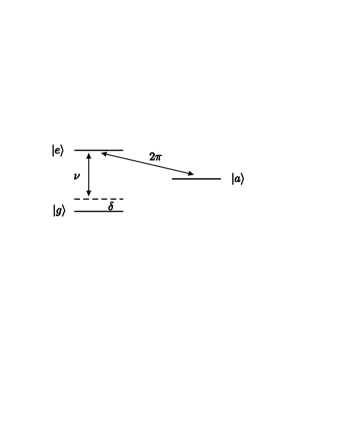
Figure 1: Diagram of a coupled two-level system subjected to ideal $2\pi$ pulses.

By applying an ideal $2\pi$ pulse (or parity kick, see Fig. 1), which is very strong in amplitude and short in time but gives a $\pi$ phase shift solely to the excited state $|e\rangle$ utilizing an auxiliary state $|a\rangle$ Agarwal et al. (2001a), the state of the system changes according to

$$x|e\rangle+y|g\rangle \underrightarrow{\;\;2\pi\;{\rm pulse}\;\;} -x|e\rangle+y|g\rangle$$ (5)

where $|x|^{2}+|y|^{2}=1$. We denote such a pulse as $Z$ pulse hereafter

$$Z(x|e\rangle+y|g\rangle)=-x|e\rangle+y|g\rangle.$$ (6)

In fact, $Z=-\sigma_{z}=|g\rangle\langle g|-|e\rangle\langle e|$.

The evolution operator for the $2\pi$ pulse and the free evolution $\tau$ is

$$U^{(1)} = ZU=\left(\begin{array}[]{cc}d_{1}&d_{2}\\ -d_{2}&-d_{1}^{*}\end{array}\right).$$ (9)

For $N$ such operations, the evolution operator at time $t=N\tau$ becomes

$$U^{(N)} = \left(\begin{array}[]{cc}d_{1}&d_{2}\\ -d_{2}&-d_{1}^{*}\end{array}\right)^{N}.$$ (12)

Let $d_{1}=d_{1r}+id_{1i}$ and $d_{2}=id_{2i}$. After some straightforward simplifications with the use of Pauli matrices, one easily obtains

$$U^{(N)} = i^{N}(\cos N\lambda-i\sigma_{\alpha}\sin N\lambda)$$ (13)

where $\sin\lambda=\sqrt{1-d_{1i}^{2}}$ and $\sigma_{\alpha}=(1/\sin\lambda)(d_{1r}\sigma_{z}-d_{2i}\sigma_{y})$. Note that $\lambda$ depends on $\tau$ instead of $t=N\tau$.

The transition probability from the initial state $|e\rangle$ to the ground state $|g\rangle$ is

$$p_{eg}^{\prime}(t=N\tau) = |\langle g|U^{(N)}|e\rangle|^{2}=p_{eg}(\tau){\sin^{2}N\lambda\over\sin^{2}\lambda}.$$ (14)

The above result is exact for any coupling strength and pulse delay $\tau$. For weak coupling $\nu\ll\delta$, $\Omega\approx\delta^{\prime}$ and $\lambda\approx\delta^{\prime}\tau+\pi/2+2k\pi$ with $k$ an integer, then

$$p_{eg}^{\prime} \approx {\nu^{2}\over\delta^{\prime 2}}\tan^{2}\delta^{\prime}\tau\sin^{2}N\delta^{\prime}\tau$$ (15)

for even $N$, which is exactly Eq. (9) in Agarwal et al.’s paper Agarwal et al. (2001a).

IV Quantum Zeno and anti-Zeno effects

The above results are applicable only to single mode bath/environment which couples to the central two-level system. In general the bath has multimodes and the coupling may depend on the mode, e.g., the dipolar coupling between an atom and an electric and magnetic field. For a many-mode bath, the transition probability of the two-level system subjected to control pulses is in general given by

$$p_{eg}^{\prime} = \sum_{n}{\nu^{2}\over\Omega_{n}^{2}}\sin^{2}\Omega_{n}\tau{\sin^{2}N\lambda_{n}\over\sin^{2}\lambda_{n}}$$ (16)

with $n$ the bath mode index mmnote . Note that $\Omega_{n}$ and $\lambda_{n}$ become mode dependent in the many-mode bath case and $\nu$ is constant here but will be considered as mode dependent in Sec. IV.4. Assuming the bath spectrum is dense, we turn the summation over mode index $n$ into the integration over mode frequency $\omega$,

$$p_{eg}^{\prime} = \int d\omega\rho(\omega){\nu^{2}\over\Omega^{2}}\sin^{2}\Omega\tau{\sin^{2}N\lambda\over\sin^{2}\lambda}$$ (17)

where $\rho(\omega)$ is the density of states of the bath. For $N=1$ we get the free decay results (no control pulse). Before considering the real physical systems which usually have mode dependent coupling, we study several toy models with constant coupling strength $\nu=\nu_{0}$ for all bath modes to gain some ideas about the effect of control pulses.

IV.1 Uniform spectrum intensity

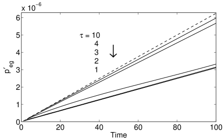
Figure 2: Control pulse effect with fixed pulse delays. The parameters are $\omega_{0}=1,\nu_{0}=0.001,\omega_{c}=100$, and $\tau=10,4,3,2,1$ from top to bottom for solid lines. The dashed line denotes the free decay. Time is in units of $1/\omega_{0}$ hereafter.

Taking $\rho(\omega)=\rho_{0}\equiv 1/\omega_{c}$ if $\omega\in[0,\omega_{c}]$ and $\rho(\omega)=0$ otherwise with $\omega_{c}$ denoting the cutoff frequency of the bath, Fig. 2 shows typical free decay and controlled decay of the excited state. Except at very short times, Fig. 2 shows that the transition probability linearly depends on the total evolution time. Utilizing the linear dependence, one defines decay rate (Einstein constant) at long time $t$ as

$$A \equiv {\partial p_{eg}(t)\over\partial t}=2\pi\rho_{0}\nu_{0}^{2}$$ (18)

for free decay Agarwal et al. (2001a) and

$$A^{\prime} \equiv {1\over\tau}{\partial p_{eg}^{\prime}\over\partial N}={2\pi\rho_{0}\nu_{0}^{2}\over\tau^{2}}\sum_{k}{1\over\nu_{0}^{2}+(\omega_{k}-\omega_{0})^{2}/4}$$ (19)

for controlled decay, where $\omega_{k}$ is the $k$th resonant mode frequency Kofman and Kurizki (2001). For weak coupling $\nu_{0}\ll\pi/\tau$, the $k$th resonant mode lies approximately at $\omega_{k}\approx\omega_{0}+(2k+1)\pi/\tau$ where $\sin\lambda\ll 1$ and $\sin 2N\lambda/\sin\lambda\approx\pi\delta(\lambda)\approx(2\pi/\tau)\delta(\omega-\omega_{k})$ for large $N$. Note that the two nearest neighbor peaks around $\omega_{0}$ with $k=0$ and $k=-1$ contribute equally about $40\%$ among all the peaks Agarwal et al. (2001a); Kofman and Kurizki (2001).

If we assume the bath has only positive frequency and concentrate on the two dominant peaks, we find

$${A^{\prime}\over A} \simeq \left\{\begin{array}[]{cc}0,&\omega_{c}\tau<\pi\\ {1/2},&\omega_{0}\tau<\pi<\omega_{c}\tau\\ 1,&{\rm otherwise}\end{array}\right.$$ (23)

and $p_{eg}^{\prime}/p_{eg}$ also shows step-like behavior as depicted in Fig. 3. Moreover, Fig. 3 exhibits only quantum Zeno effect, i.e., suppression of the decay by the control pulses. The decay are completely suppressed, $A^{\prime}=0$, once the control pulse frequency is larger than the cutoff frequency.

Figure 3: (Color online) Control pulse effect vs number of pulses $N$ (main panel) and relative positions of resonant modes to $\omega_{0}$ and $\omega_{c}$ (upper three panels A, B, and C corresponds to three regions in the main panel, respectively). The parameters are $N\tau=100,\omega_{0}=1,\nu_{0}=0.001$, and $\omega_{c}=100$. Two big steps shows two major peaks out of the lower and upper cutoff frequency, respectively. These small steps shows minor peaks going out of the cutoff frequencies. Circles are for the frequency-dependent coupling case.

IV.2 Gaussian spectrum intensity

A Gaussian spectrum intensity has a form as

$$\rho(\omega) = {1\over\sqrt{2\pi}\;\Gamma}\;e^{-(\omega-\omega_{m})^{2}/2\Gamma^{2}},\;\;\omega\geq 0$$ (24)

where $\Gamma$ and $\omega_{m}$ denotes the width and the position of the maximal intensity, respectively.

IV.2.1 $\omega_{0}=\omega_{m}$

In this case we expect only quantum Zeno effect to appear, $A^{\prime}\leq A$, because it is easy to check that

$${A^{\prime}\over A} = {4\over\pi^{2}}\sum_{k}{1\over(2k+1)^{2}}\;{\rho(\omega_{k})\over\rho(\omega_{0})}\leq 1$$ (25)

where we have used the large $N$ and weak coupling assumptions. By considering the two dominant peaks, we further obtain that

$${A^{\prime}\over A} \approx {8\over\pi^{2}}\;e^{-\pi^{2}/2\Gamma^{2}\tau^{2}}$$ (26)

for small $\tau$ such that $\Gamma\tau\lesssim\pi$. Equation (26) shows that the decay rate decreases rapidly with the control pulse frequency in a Gaussian form. For exceedingly small $\tau$ which satisfies $\Gamma\tau\ll\pi$, $A^{\prime}$ is essentially zero, which means the transition is inhibited and the survival probability of the initial state saturates. The red dashed line in Fig. 4 demonstrates the quantum Zeno effect and the prohibition of the transition.

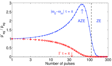
Figure 4: (Color online) Reduced transition probability at fixed time ($t=N\tau=100$) vs number of pulses $N$ for Gaussian spectrum intensity for $\omega_{0}=\omega_{m}$ (red dashed line) and $\omega_{0}=\omega_{m}-2$ (blue solid line). Circles and crosses are for the corresponding frequency-dependent coupling case. The vertical dot-dashed line shows the boundary between quantum Zeno and anti-Zeno effects for $\omega_{0}=\omega_{m}-2$. Other parameters are $\nu_{0}=0.001,\omega_{c}=100,\omega_{m}=\omega_{c}/2$, $\Gamma=1$.

IV.2.2 $|\omega_{0}-\omega_{m}|\gtrsim\Gamma$

For $|\omega_{0}-\omega_{m}|<\Gamma$, the results are similar to $\omega_{0}=\omega_{m}$ and exhibit only quantum Zeno effect. To observe substantially enhancement of the transition, i.e., the quantum anti-Zeno effect Kofman and Kurizki (2000), $|\omega_{0}-\omega_{m}|\gtrsim\Gamma$ is required. More specifically, by taking the biggest peak around $\omega_{0}$, one obtains the necessary condition for quantum anti-Zeno effect as

$$|\omega_{0}-\omega_{m}|\geq\sqrt{4\ln{\pi\over 2}}\;\Gamma\approx 1.3\Gamma.$$ (27)

The blue solid line in Fig. 4 shows the quantum Zeno and anti-Zeno effects for $|\omega_{0}-\omega_{m}|=2$. Both quantum Zeno (large $N$ region) and anti-Zeno (small $N$ region) effects are observed. At fixed time $t=N\tau$, large $\tau$ (small N) gives anti-Zeno effect while small $\tau$ (large N) gives Zeno effect. The boundary between quantum Zeno and anti-Zeno effect is about $2|\omega_{m}-\omega_{0}|\tau\approx\pi$ if $|\omega_{m}-\omega_{0}|\gg\Gamma$. Strongest anti-Zeno effect is obtained at $|\omega_{0}-\omega_{m}|\tau=\pi$ where one of the two main resonant modes lies near $\omega_{m}$.

IV.3 Lorentzian and exponential spectrum intensity

The spectrum intensity for Lorentzian and exponential are, respectively,

$$\rho(\omega) = {\Gamma/\pi\over(\omega-\omega_{m})^{2}+\Gamma^{2}},\;\omega\geq 0$$ (28)

$$\rho(\omega) = {1\over 2\Gamma}e^{-|\omega-\omega_{m}|/\Gamma},\;\omega\geq 0.$$ (29)

Similar to Gaussian spectral intensity, only the quantum Zeno effect is observed if $\omega_{0}=\omega_{m}$ for the Lorentzian and exponential shape (Fig. 5). The transition probability is essentially inhibited once $\tau\ll\tau_{c}$ where $\tau_{c}\sim 1/\omega_{c}$. Once $|\omega_{0}-\omega_{m}|\gtrsim\Gamma$, we find both quantum Zeno and anti-Zeno effects and the boundary between Zeno and anti-Zeno regime is determined approximately by $2|\omega_{m}-\omega_{0}|\tau\approx\pi$. The peak position of the quantum anti-Zeno effect lies about at $|\omega_{0}-\omega_{m}|\tau\approx\pi$. As shown in Fig. 5, the reduced transition probability in the exponential case has a narrower peak width than that in the Lorentzian case. Two small secondary peaks are noticeable in the anti-Zeno region of the exponential spectrum case. These peaks are due to the second and third quasi-level resonant to $\omega_{m}$. They satisfy the condition, respectively, $|\omega_{0}-\omega_{m}|\tau\approx 3\pi,5\pi$.

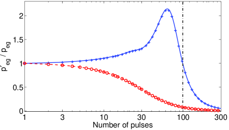
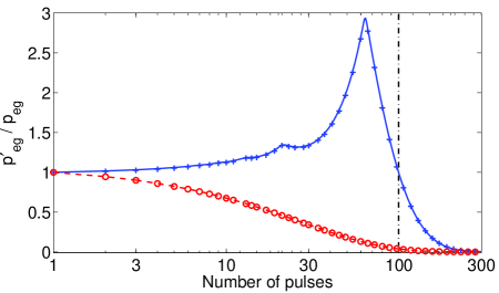
Figure 5: (Color online) Same as Fig. 4 except that the spectrum intensity is Lorentzian (top) and exponential (bottom).

IV.4 Frequency dependent coupling

The widely adopted dipolar coupling in spontaneous emission of a two level atom or molecule has a frequency dependence as $\nu(\omega)=\nu_{0}\sqrt{\omega}$ where $\nu_{0}$ is taken as a constant, which depends on the dipole matrix elements Scully and Zubairy (1997). We will consider the same coupling spectrum intensity as before, i.e.,

$$\rho(\omega) = {1\over\omega}{1\over\sqrt{2\pi}\;\Gamma}\;e^{-(\omega-\omega_{m})^{2}/2\Gamma^{2}},\;\omega\geq 0$$ (30)

$$\rho(\omega) = {1\over\omega}{\Gamma/\pi\over(\omega-\omega_{m})^{2}+\Gamma^{2}},\;\omega\geq 0$$ (31)

$$\rho(\omega) = {1\over\omega}{1\over 2\Gamma}e^{-|\omega-\omega_{m}|/\Gamma},\;\omega\geq 0$$ (32)

for Gaussian, Lorentzian, and exponential density of state, respectively. As shown in Figs. 4 and 5, the frequency dependent coupling has little effect on the performance of the control pulses.

V Decay freezing

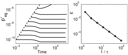
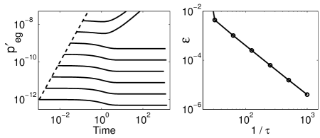
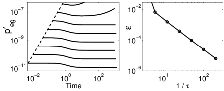
Figure 6: Decay freezing (left column) and dependence of the differential freezing value on pulse delay (right column) for the Gaussian (top row), Lorentzian (middle row), and exponential (bottom row) spectrum. Only results of odd number pulses are plotted for a better view. The dashed lines show decay without control pulses. Crosses of dashed lines and solid lines in the left column panels denote the specific pulse delay $\tau$.

By inspecting Eq. (17), the controlled transition probability freezes if $N\lambda\gg 1$ and the freezing value is

$$\lim_{N\rightarrow\infty}p_{eg}^{\prime} = {1\over 2}\int d\omega\rho(\omega){\nu^{2}\over\Omega^{2}}\sin^{2}\Omega\tau{1\over\sin^{2}\lambda},$$ (33)

where we have replaced the rapidly oscillating integrand $\sin^{2}(N\lambda)$ with its average $1/2$. The left column of Fig. 6 from numerical calculation indeed shows that the transitions freeze at long times for three different cases at small $\tau$. The smaller the $\tau$ is, the smaller the freezing value is. Freezing of the transition probability is equivalent to freezing of the survival probability of the excited state, $f=1-p^{\prime}_{eg}$.

Moreover, for small enough pulse delay $\tau$, we have $\sin^{2}\lambda\approx 1$ thus

$$\lim_{N\rightarrow\infty}p_{eg}^{\prime} \approx {1\over 2}\int d\omega\rho(\omega){\nu^{2}\over\Omega^{2}}\sin^{2}\Omega\tau={1\over 2}p_{eg}(\tau).$$ (34)

The above relation indicates that the freezing value of the transition probability at long times is one half of the free transition value at $t=\tau$ which is the pulse delay. Clearly, the road map to the quantum ZE is that the decay rate becomes zero after initial pulses (decay freezing) and the freezing value of the survival probability $f$ approaches 1 as $\tau$ decreases.

Define differential freezing value $\varepsilon(\tau)=p_{eg}^{\prime}(N\tau=1000)-{1\over 2}p_{eg}(\tau)$, which describes the difference of the transition probability after many pulses and one half of the decay in the first pulse delay. The right column of Fig. 6 shows that $\varepsilon$ decreases with increasing of $1/\tau$ (decreasing of $\tau$), confirming the analytical results of Eq. (34).

In fact, decay freezing exists not only in the model system we consider in the paper, but also exists in many other pulse-controlled systems, such as gated semiconductor quantum dot Zhang et al. (2007a, b, 2008); Lee et al. (2008); Liu et al. (2007), spin-boson model Viola and Lloyd ; Faoro and Viola (2004), and nuclear spins Haeberlen (1976). The basic idea behind the decay freezing is that the control pulses creates an effective preferred direction along which the decay is frozen. In terms of Pauli matrix (c.f. Eq. 2), the preferred direction created by control pulses in the model we consider is $z$.

VI Conclusion and discussion

By investigating three models of coupling spectrum intensity (Gaussian, Lorentzian and exponential), we demonstrate that a two-level system subjected to many ideal $2\pi$ pulses exhibits both quantum Zeno and anti-Zeno effect, depending on the relative position of $\omega_{0}$ to the peak position $\omega_{m}$ of the spectrum and the pulse delay $\tau$. Instead of decreasing the decay rate, the pulsed two-level system shows decay freezing after many pulses at small $\tau$ and the freezing value of the survival probability of the initial excited state approaches 1 (no decay) with decreasing $\tau$.

In this paper, all the spectrums have single peak and we observe only single quantum Zeno and/or anti-Zeno region. Under some special circumstances where a multiple peaks spectrum exists, one would expect multiple quantum Zeno and anti-Zeno regions. We have also assumed that the spectrum of the structured vacuum is time independent where the back action exerted on the vacuum by the two-level system has been neglected. A full quantum version of the coupling between the two-level system and the vacuum could possibly change the picture of the controlled decay at long times but the short time behavior would be intact in the weak coupling regime, because the back action is weak and needs a long time to manifest its effect on the two-level system dynamics.

We consider only periodic pulse sequence ($\tau$ is fixed) in this paper. In principle, other pulse sequences with varying $\tau$ may also give similar quantum Zeno and anti-Zeno effect. They may even have additional advantages Uhrig (2007); Lee et al. (2008). In addition, the strength and the duration of the $2\pi$ pulses are finite in practice. One could minimize the finite pulse effect by employing the phase alternation techniques Slichter (1992) or the Eulerian protocols Viola (2004).

VII Acknowledgments

W. Z. is grateful for many helpful discussions with V. V. Dobrovitski, S. Y. Zhu, and T. Yu. This work was partially carried out at the Ames Laboratory, which is operated for the U. S. Department of Energy by Iowa State University under Contract No. W-7405-82 and was supported by the Director of the Office of Science, Office of Basic Energy Research of the U. S. Department of Energy. Part of the calculations was performed at the National High Performance Computing Center of Fudan University.

References

- Milonni (1994) P. W. Milonni, The Quantum Vacuum: An Introduction to Quantum Electrodynamics (Academic Press, New York, 1994).
- Scully and Zubairy (1997) M. O. Scully and M. S. Zubairy, Quantum Optics (Cambridge University Press, Cambridge, 1997).
- Allen and Eberly (1975) L. Allen and J. H. Eberly, Optical Resonance and Two-level Atoms (Dover Publication, New York, 1975).
- Frishman and Shapiro (2003) E. Frishman and M. Shapiro, Phys. Rev. A 68, 032717 (2003).
- Evers and Keitel (2002) J. Evers and C. H. Keitel, Phys. Rev. Lett. 89, 163601 (2002).
- Frishman and Shapiro (2001) E. Frishman and M. Shapiro, Phys. Rev. Lett. 87, 253001 (2001).
- Agarwal et al. (2001a) G. S. Agarwal, M. O. Scully, and H. Walther, Phys. Rev. Lett. 86, 4271 (2001a).
- Vogel and Welsch (2006) W. Vogel and D.-G. Welsch, Quantum Optics (Wiley-VCH, Weinheim, 2006), 3rd ed.
- Itano et al. (1990) W. M. Itano, D. J. Heinzen, J. J. Bollinger, and D. J. Wineland, Phys. Rev. A 41, 2295 (1990).
- Itano et al. (1991) W. M. Itano, D. J. Heinzen, J. J. Bollinger, and D. J. Wineland, Phys. Rev. A 43, 5168 (1991).
- Misra and Sudarshan (1977) B. Misra and E. C. G. Sudarshan, J. Math. Phys. 18, 756 (1977).
- Kofman and Kurizki (2000) A. G. Kofman and G. Kurizki, Nature(London) 405, 546 (2000).
- Agarwal et al. (2001b) G. S. Agarwal, M. O. Scully, and H. Walther, Phys. Rev. A 63, 044101 (2001b).
- Fischer et al. (2001) M. C. Fischer, B. Gutiérrez-Medina, and M. G. Raizen, Phys. Rev. Lett. 87, 040402 (2001).
- Kofman and Kurizki (2001) A. G. Kofman and G. Kurizki, Phys. Rev. Lett. 87, 270405 (2001).
- Scully et al. (2003) M. O. Scully, S.-Y. Zhu, and M. S. Zubairy, Chaos, Solitons and Fractals 16, 403 (2003).
- (17) We have assumed the dipolar interaction has a symmetry such that , where and are the dipole operator of the atom and the electric field of the light, respectively.
- (18) We adopt the Schrödinger picture instead of the usual interaction picture (e.g., Ref. Agarwal et al. (2001a)) for our convenience. Both pictures are equivalent in principle.
- (19) For weak couplings, which are the case in the decay problem we consider, high order nonlinear interaction between the two-level atom and multiple electric field modes is neglected.
- Zhang et al. (2007a) W. Zhang, V. V. Dobrovitski, L. F. Santos, L. Viola, and B. N. Harmon, Phys. Rev. B 75, 201302(R) (2007a).
- Zhang et al. (2007b) W. Zhang, N. P. Konstantinidis, K. A. Al-Hassanieh, and V. V. Dobrovitski, J. Phys.: Condens. Matter 19, 083202 (2007b).
- Zhang et al. (2008) W. Zhang, N. P. Konstantinidis, V. V. Dobrovitski, B. N. Harmon, L. F. Santos, and L. Viola, Phys. Rev. B 77, 125336 (2008).
- Lee et al. (2008) B. Lee, W. M. Witzel, and S. Das Sarma, Phys. Rev. Lett. 100, 160505 (2008).
- Liu et al. (2007) R.-B. Liu, W. Yao, and L. J. Sham, New J. Phys. 9, 226 (2007).
- (25) L. Viola and S. Lloyd, eprint quant-ph/9809058.
- Faoro and Viola (2004) L. Faoro and L. Viola, Phys. Rev. Lett. 92, 117905 (2004).
- Haeberlen (1976) U. Haeberlen, High resolution NMR in solids: Selective averaging (Academic Press, New York, 1976).
- Uhrig (2007) G. S. Uhrig, Phys. Rev. Lett. 98, 100504 (2007).
- Slichter (1992) C. P. Slichter, Principles of Magnetic Resonance (Springer-Verlag, New York, 1992).
- Viola (2004) L. Viola, J. Mod. Opt. 51, 2357 (2004).