A method for reconstructing the variance of a 3D physical field from 2D observations: Application to turbulence in the ISM

Abstract

We introduce and test an expression for calculating the variance of a physical field in three dimensions using only information contained in the two-dimensional projection of the field. The method is general but assumes statistical isotropy. To test the method we apply it to numerical simulations of hydrodynamic and magnetohydrodynamic turbulence in molecular clouds, and demonstrate that it can recover the 3D normalised density variance with $\sim$ 10% accuracy if the assumption of isotropy is valid. We show that the assumption of isotropy breaks down at low sonic Mach number if the turbulence is sub-Alfvénic. Theoretical predictions suggest that the 3D density variance should increase proportionally to the square of the Mach number of the turbulence. Application of our method will allow this prediction to be tested observationally and therefore constrain a large body of analytic models of star formation that rely on it.

1 Introduction

It is a fundamental problem in astrophysics that we typically only have access to two-dimensional (2D) physical fields that have been integrated or averaged over the line-of-sight, while the physical fields of interest are intrinsically three-dimensional (3D). Constraining 3D properties is very difficult, and is limited to structures with a fairly simple geometry (e.g. Lucy 1974 – see Reblinsky 2000 for an application to galaxy clusters). Molecular clouds have very complex structure that is not suitable for direct inversion from 2D to 3D, but there exist methods for inferring statistical information on the scaling behaviour of the 3D structure of the density and velocity fields (e.g. Stutzki et al 1998). Molecular cloud evolution is driven in large part by the action of turbulence, and recently, much interest has been directed towards the action of turbulence in shaping the density field in molecular clouds, in particular towards the theoretically predicted increase in the variance of the density field with the Mach number of the turbulence (Padoan, Nordlund, & Jones 1997; Passot & Vázquez-Semadeni 1998). This prediction plays a key role in analytic models of star formation (Padoan & Nordlund 2002; Krumholz & McKee 2005; Elmegreen 2008; Hennebelle & Chabrier 2008; Padoan & Nordlund 2009; Hennebelle & Chabrier 2009).

If the density, $\rho$, is expressed in units of the mean density, $\rho_{0}$, the theoretical predictions for the relationship between the density variance and root mean square (rms) Mach number, $M$, may be simply written as:

$$\sigma_{\rho/\rho_{0}}^{2}\;=\;b^{2}M^{2},$$ (1)

where $b$ is a constant of proportionality. In the case of isothermal gas, which is applicable to a good approximation to molecular clouds, the probability density function (PDF) of the density field is thought to be lognormal in form (Vázquez-Semadeni 1994). Using a lognormal form for the density PDF, Padoan & Nordlund (2002) derive a relation between the variance in the logarithm of the density field, $\sigma_{\ln{(\rho/\rho_{0}})}^{2}$, and the rms Mach number, $M$:

$$\sigma_{\ln{(\rho/\rho_{0}})}^{2}=\ln{(1+b^{2}M^{2})},$$ (2)

which is equivalent to equation (1). A range of predictions for $b$ have been proposed, which were recently synthesized into a unified model by Federrath et al (2008) who propose that $b=1/3$ for solenoidal (divergence-free) forcing and $b=1$ for compressive (curl-free) forcing in 3D.

Given the importance of equation (1) for analytic models of star formation, it is essential to test it with observational data. Initial observational tests by Goodman, Pineda, & Schnee (2009) did not find any obvious support for the theoretical predictions. Federrath et al (2009) have suggested a reason for this lack of agreement, citing variations in $b$ caused by different turbulent forcing mechanisms. Perhaps more importantly, these observations relied on measuring the variance in the projected 2D column density rather than in the 3D density field that appears in the theoretical predictions. From observations, we do not have access to the 3D density and velocity fields to directly test this prediction, and evaluate its applicability to molecular clouds and to the predictive star formation models.

In this paper, we derive and test an expression that relates the observable variance in the 2D column density field to the true 3D variance of the density field. The method is completely general, albeit with the assumption of statistical isotropy, and may also be applied to the projection of other physical fields. In Section 2, we present the analytical expressions needed to convert the 2D variance into the 3D variance. In Section 3, we demonstrate the application of the method to numerical simulations of hydrodynamic and magnetohydrodynamic turbulence. Our summary is given in Section 4.

2 The Statistics of Projection from 3D to 2D

2.1 Development of the Method

Given a physical field in 3D, we wish to examine how the statistical properties of a 2D projected field are related to the intrinsic properties. By doing this, we can then infer intrinsic quantities from the measureable quantities. We focus here on the variance, measured in 3D and in projected 2D. In our initial derivation, we consider a 3D field, $F_{3}(x,y,z)$, which is averaged along the $z$ axis to produce a projected field $F_{2}(x,y)$, via:

$$F_{2}(x,y)={\frac{1}{L}}\int_{-L/2}^{L/2}dz\;F_{3}(x,y,z)$$ (3)

where $L$ is the physical size of the region, assumed cubical, that contains $F_{3}$.

We will make use of the 3D Fourier series of $F_{3}$, obtained over the interval $[-L/2,+L/2]$, which is:

$$\tilde{F_{3}}({\textbf{{k}}})=\displaystyle\int_{-L/2}^{L/2}\displaystyle\int_{-L/2}^{L/2}\displaystyle\int_{-L/2}^{L/2}\;d^{3}\textbf{{{{r}}}}\;F_{3}({\textbf{{r}}})\;e^{-2\pi i{\textbf{{k}}}\cdot{\textbf{{r}}}/L}$$ (4)

where $\textbf{{{{r}}}}=(x\hat{\textbf{{x}}},y\hat{\textbf{{y}}},z\hat{\textbf{{z}}})$ and the spatial frequencies are $\textbf{{k}}=(k_{x}\hat{\textbf{{x}}},k_{y}\hat{\textbf{{y}}},k_{z}\hat{\textbf{{z}}})$, for integer $k_{x}$, $k_{y}$, and $k_{z}$. The field $F_{3}$ can then be written as:

$${F_{3}}({\textbf{{r}}})={\frac{1}{L^{3}}}\displaystyle\sum_{k_{x}=-\infty}^{\infty}\sum_{k_{y}=-\infty}^{\infty}\sum_{k_{z}=-\infty}^{\infty}\;\tilde{F_{3}}(k_{x},k_{y},k_{z})\;e^{2\pi i{\textbf{{k}}}\cdot{\textbf{{r}}}/L}.$$ (5)

Inserting equation (5) into equation (3),

$$F_{2}(x,y)=$$

$${\frac{1}{L^{4}}}\displaystyle\int_{-L/2}^{L/2}dz\displaystyle\sum_{k_{x}=-\infty}^{\infty}\sum_{k_{y}=-\infty}^{\infty}\sum_{k_{z}=-\infty}^{\infty}\tilde{F_{3}}(k_{x},k_{y},k_{z})\;e^{2\pi i{\textbf{{k}}}\cdot{\textbf{{r}}}/L}$$ (6)

and computing the $z$ integral first, we find that:

$$F_{2}(x,y)={\frac{1}{L^{3}}}\displaystyle\sum_{k_{x}=-\infty}^{\infty}\sum_{k_{y}=-\infty}^{\infty}\tilde{F_{3}}(k_{x},k_{y},k_{z}=0)\;e^{2\pi i{\textbf{{k}}}\cdot{\textbf{{r}}}/L},$$ (7)

since

$${\frac{1}{L}}\int_{-L/2}^{L/2}dz\;e^{2\pi ik_{z}z/L}=1\;\;{\mathrm{for}}\;\;k_{z}=0,$$ (8)

$${\frac{1}{L}}\int_{-L/2}^{L/2}dz\;e^{2\pi ik_{z}z/L}=0\;\;{\mathrm{for}}\;\;k_{z}\neq 0.$$ (9)

Since the 2D Fourier series, over the interval $[-L/2,+L/2]$, of $F_{2}$ is:

$$\tilde{F_{2}}({\textbf{{k${}_{2}$}}})=\displaystyle\int_{-L/2}^{L/2}\displaystyle\int_{-L/2}^{L/2}\;d^{2}{\textbf{{r${}_{2}$}}}\;F_{2}({\textbf{{r${}_{2}$}}})\;e^{-2\pi i{\textbf{{k${}_{2}$}}}\cdot{\textbf{{r${}_{2}$}}}/L}$$ (10)

where $\textbf{{{{r${}_{2}$}}}}=(x\hat{\textbf{{x}}},y\hat{\textbf{{y}}})$ and $\textbf{{k${}_{2}$}}=(k_{x}\hat{\textbf{{x}}},k_{y}\hat{\textbf{{y}}})$, and:

$${F_{2}}({\textbf{{r${}_{2}$}}})={\frac{1}{L^{2}}}\displaystyle\sum_{k_{x}=-\infty}^{\infty}\sum_{k_{y}=-\infty}^{\infty}\tilde{F_{2}}(k_{x},k_{y})\;e^{2\pi i{\textbf{{k${}_{2}$}}}\cdot{\textbf{{r${}_{2}$}}}/L},$$ (11)

we see that, comparing equation (7) and equation (11):

$$\tilde{F_{2}}(k_{x},k_{y})={\frac{1}{L}}\tilde{F_{3}}(k_{x},k_{y},k_{z}=0).$$ (12)

In other words: the 2D Fourier series of $F_{2}$ is proportional to the $k_{z}=0$ cut through $\tilde{F_{3}}$. Previous studies have made use of this result (e.g. Stutzki et al. 1998; Lazarian & Pogosyan 2000; Brunt & Mac Low 2004; Miville-Deschenes & Martin (2007)). As the power spectrum, $P_{3}({\textbf{{k}}})$, is the squared modulus of the Fourier transform ($P_{3}({\textbf{{k}}})=\tilde{F_{3}}({\textbf{{k}}})\tilde{F_{3}}^{*}({\textbf{{k}}})$), 2D power spectra of projected fields have been used to infer the 3D power spectrum, under the assumption of isotropy, i.e. that the $k_{z}=0$ cut through the power spectrum is statistically representive of the full power spectrum. In our analysis below, we will also make use of the power spectrum and the assumption of isotropy.

Now we compute the variances in the 3D and 2D fields. From the mean value of $F_{3}$:

$$\langle{F_{3}}\rangle={\frac{1}{L^{3}}}\displaystyle\int_{-L/2}^{L/2}\displaystyle\int_{-L/2}^{L/2}\displaystyle\int_{-L/2}^{L/2}\;d^{3}{\textbf{{r}}}\;F_{3}({\textbf{{r}}}),$$ (13)

and the mean square value of $F_{3}$:

$$\langle{F_{3}^{2}}\rangle={\frac{1}{L^{3}}}\displaystyle\int_{-L/2}^{L/2}\displaystyle\int_{-L/2}^{L/2}\displaystyle\int_{-L/2}^{L/2}\;d^{3}{\textbf{{r}}}\;F_{3}^{2}({\textbf{{r}}}),$$ (14)

we find the variance of $F_{3}$ as:

$$\sigma_{3}^{2}=\langle{F_{3}^{2}}\rangle-\langle{F_{3}}\rangle^{2}.$$ (15)

We also make use of the Fourier transform of $F_{3}$, by noting that:

$$\langle{F_{3}}\rangle={\frac{1}{L^{3}}}\tilde{F_{3}}(0,0,0)$$ (16)

and, through Parseval’s Theorem:

$$\langle{F_{3}^{2}}\rangle={\frac{1}{L^{6}}}\displaystyle\sum_{k_{x}=-\infty}^{\infty}\sum_{k_{y}=-\infty}^{\infty}\sum_{k_{z}=-\infty}^{\infty}\;\tilde{F_{3}}\tilde{F_{3}}^{*},$$ (17)

allowing us to rewrite equation (15) as:

$$\sigma_{3}^{2}={\frac{1}{L^{6}}}\left(\left(\displaystyle\sum_{k_{x}=-\infty}^{\infty}\sum_{k_{y}=-\infty}^{\infty}\sum_{k_{z}=-\infty}^{\infty}\;\tilde{F_{3}}\tilde{F_{3}}^{*}\right)-\tilde{F_{3}}^{2}(0,0,0)\right).$$ (18)

By similar analysis, we find the variance of $F_{2}$ is:

$$\sigma_{2}^{2}={\frac{1}{L^{4}}}\left(\left(\displaystyle\sum_{k_{x}=-\infty}^{\infty}\sum_{k_{y}=-\infty}^{\infty}\;\tilde{F_{2}}\tilde{F_{2}}^{*}\right)-\tilde{F_{2}}^{2}(0,0)\right),$$ (19)

or, applying equation (12):

$$\sigma_{2}^{2}={\frac{1}{L^{6}}}\times$$

$$\left(\left(\displaystyle\sum_{k_{x}=-\infty}^{\infty}\sum_{k_{y}=-\infty}^{\infty}\;\tilde{F_{3}}(k_{z}=0)\tilde{F_{3}}^{*}(k_{z}=0)\right)-\tilde{F_{3}}^{2}(0,0,0)\right).$$

(20)

The ratio, $R$, of the variance of $F_{2}$ to the variance of $F_{3}$ is therefore:

$$\frac{\sigma_{2}^{2}}{\sigma_{3}^{2}}=R=$$

$$\frac{\left(\displaystyle\sum_{k_{x}=-\infty}^{\infty}\sum_{k_{y}=-\infty}^{\infty}\;\tilde{F_{3}}(k_{z}=0)\tilde{F_{3}}^{*}(k_{z}=0)\right)-\tilde{F_{3}}^{2}(0,0,0)}{\left(\displaystyle\sum_{k_{x}=-\infty}^{\infty}\sum_{k_{y}=-\infty}^{\infty}\sum_{k_{z}=-\infty}^{\infty}\;\tilde{F_{3}}\tilde{F_{3}}^{*}\right)-\tilde{F_{3}}^{2}(0,0,0)}$$ .

(21)

In practice, the measureable physical fields, either through observations or numerical simulations, will consist of a discrete number of measurements at a fixed set of grid points. We define the scale ratio, $\lambda$, as the ratio of the image (or cube) size to the pixel size. Taking the grid to be of size $\lambda\times\lambda\times\lambda$ or $\lambda\times\lambda$ pixels in 3D and 2D respectively, the Fourier transforms are carried out at a discrete set of spatial frequencies, $k=-\lambda/2+1,-\lambda/2+2,...,-2,-1,0,1,2...,\lambda/2-1,\lambda/2$ along each axis. The quantity $\tilde{F_{3}}\tilde{F_{3}}^{*}$ is the spectral power, $P_{3}$, which can be observationally derived (up to an unimportant constant of proportionality) as follows. If we had a projected mean 2D field, $F_{2}$, and wanted to use this to infer the 3D variance, then we would compute its power spectrum, $P_{2}(k_{x},k_{y})$, and from this produce an azimuthally-averaged power spectrum $P_{2}(k)$, which depends only on the modulus of the spatial frequency, $k$. The key idea behind the method is that we can, assuming isotropy, take:

$$P_{3}(k)\propto P_{2}(k),$$ (22)

to obtain:

$$R=\frac{\left(\displaystyle\sum_{k_{x}=-\lambda/2+1}^{\lambda/2}\sum_{k_{y}=-\lambda/2+1}^{\lambda/2}P_{2}(k)\right)-P_{2}(0)}{\left(\displaystyle\sum_{k_{x}=-\lambda/2+1}^{\lambda/2}\sum_{k_{y}=-\lambda/2+1}^{\lambda/2}\sum_{k_{z}=-\lambda/2+1}^{\lambda/2}P_{2}(k)\right)-P_{2}(0)},$$ (23)

The 3D variance can then be calculated as $\sigma_{3}^{2}=\sigma_{2}^{2}/R$. Note however that since $\lambda$ is necessarily finite, the observed 2D variance and the calculated 3D variance are lower limits to the true variances that would be obtained in the limit $\lambda\longrightarrow\infty$. This is discussed further below.

A more compact form of equation (23) can be obtained by defining:

$${\displaystyle\sum_{k\neq 0}}^{2D,\lambda}P_{2}(k)=\left(\displaystyle\sum_{k_{x}=-\lambda/2+1}^{\lambda/2}\sum_{k_{y}=-\lambda/2+1}^{\lambda/2}P_{2}(k)\right)-P_{2}(0)$$ (24)

and:

$${\displaystyle\sum_{k\neq 0}}^{3D,\lambda}P_{2}(k)=$$

$$\left(\displaystyle\sum_{k_{x}=-\lambda/2+1}^{\lambda/2}\sum_{k_{y}=-\lambda/2+1}^{\lambda/2}\sum_{k_{z}=-\lambda/2+1}^{\lambda/2}P_{2}(k)\right)-P_{2}(0)$$

(25)

so that:

$$R=\frac{{\displaystyle\sum_{k\neq 0}}^{2D,\lambda}P_{2}(k)}{{\displaystyle\sum_{k\neq 0}}^{3D,\lambda}P_{2}(k)}$$ (26)

For this method to work, it is essential that the projected field, $F_{2}$, is the line-of-sight average of the 3D field, $F_{3}$ (see equation (3)). In many instances, the projected 2D field is the line-of-sight intregral of the 3D field (e.g. column density versus density). A simple solution for integrated fields that ensures the above requirements are satisfied is to express the field $F_{2}$ in normalised units – i.e. by dividing $F_{2}$ by its mean value. In this case, the variance of the normalised 3D density field can be calculated from the variance of the normalised 2D column density field, as discussed below in Section 2.6.

2.2 Approximations

The power spectra of many fields of interest are power-law in form: $P_{3}\propto k^{-\alpha}$. If the power spectrum is steep (large $\alpha$) then the variance is sensitively dependent on the power at low spatial frequencies. Because of the quantisation in equation (26) and the small amount of information available at low $k$, the above procedure may be inaccurate for large $\alpha$. Brunt & Mac Low (2004) examined 3D and projected 2D standard deviations in the normalised density field ($\rho/\rho_{0}$) and normalised column density field ($N/N_{0}$) obtained from numerical simulations, with $\lambda=128$. The (column) density power spectra were reasonably well fitted by $P_{3}(k)\propto k^{-3}$, albeit with some curvature. They found that $\sigma_{N/N_{0}}/\sigma_{\rho/\rho_{0}}\approx 0.34\pm 0.04$. Evaluating equation (26), using $\lambda=128$ and $P_{3}(k)\propto k^{-3}$, to compute the ratio of standard deviations (i.e. $\sqrt{R}$), we predict $\sigma_{2}/\sigma_{3}=0.39$, which is in acceptable agreement with the Brunt & Mac Low (2004) experimental result, given the spectral curvature.

With a power law form for the power spectrum, it is tempting to approximate equation (26) with simple integral-based expressions for $R$. If the spectral slope is $\alpha$ we could write:

$$R=\frac{2\pi\int_{1}^{\lambda/2}\;dk\;k\;k^{-\alpha}}{4\pi\int_{1}^{\lambda/2}\;dk\;k^{2}\;k^{-\alpha}},$$ (27)

which is easily solved for a specified $\alpha$. However, this is not a terribly good approximation as the integrals have been computed over circular and spherical regions of $k$-space rather than the square and cubical regions which contain the fields. At low $\alpha$ this is not sufficiently accurate, and in general we recommend that the direct summation method presented in equation (26) be used. As a trivial example, for a cube of Gaussian noise ($\alpha=0$), equation (26) correctly predicts $R=(\lambda^{2}-1)/(\lambda^{3}-1)$, which tends to $1/\lambda$ for large $\lambda$. In the same limit, equation (27) incorrectly predicts $R=3/2\lambda$. Equation (27) is useful however in gaining some intuitive understanding of how $R$ depends on the form of the power spectrum: $R$ decreases if proportionally more power resides at large $k$ because the denominator is weighted by $k^{2}$ and the numerator by $k$. The physical effect underlying this is that, if the variance is mostly at high $k$ (small spatial scales), line-of-sight averaging suppresses more of the power than if the variance is mostly at low $k$ (large spatial scales). Equation (27) is also useful for exploring scale-dependence effects on the calculated variances. Note that for $2<\alpha\leq 3$, the 2D variance converges as $\lambda\longrightarrow\infty$ but the 3D variance diverges!

2.3 Application to Observational Data

For fields acquired through observations, it is necessary to account for the telescope’s beam response (point spread function) in the calculation of variances. The observational version of equation (26) is:

$$R=\frac{{\displaystyle\sum_{k\neq 0}}^{2D,\lambda}P_{2}(k)\tilde{B}^{2}(k)}{{\displaystyle\sum_{k\neq 0}}^{3D,\lambda}P_{2}(k)\tilde{B}^{2}(k)}$$ (28)

where $\lambda$ is the number of pixels along each axis, $\tilde{B}^{2}(k)=\tilde{B}(k)\tilde{B}^{*}(k)$ is the square of the Fourier space representation of the telescope beam pattern, and $P_{2}(k)$ is the power spectrum of $F_{2}$ in the absence of beam-smoothing and instrumental noise. (Note that the observable quantity is $P_{2}(k)\tilde{B}^{2}(k)+P_{2N}(k)$ where $P_{2N}(k)$ is the noise power spectrum.) Equation (28) includes accounting for the fact that the observed variance in the 2D field has been suppressed by the smoothing imposed by the telescope beam, and this must be taken into account. In equation (28), we have also applied the beam pattern to the denominator (representing the 3D variance). This procedure may at first appear an odd choice, but it is motivated by the requirement that we limit our knowledge of the 3D variance to the resolution provided by the data. In effect, equation (28) is an attempt to construct a 3D beam that samples the 3D density field and affords the same effective linear resolution as that provided by the telescope beam in projected 2D. The Fourier series $\tilde{F}_{3}$ extends to $k=\infty$, or at least to a (potentially very large) spatial frequency, $k_{c}$, beyond which there are no variations in the field. In other words, there will be fluctuations in the projected 2D field (and therefore the 3D field) that we are not directly sensitive to, as they lie below our resolution limit. These, naturally, are additional sources of variance that we cannot measure.

The full variance of the field $F_{3}$ should in principle be derived by removing (from the denominator) the effect of the beam pattern, and summing over the spatial frequency range $1\leq k\leq k_{c}$. In general, we will have little or no information about $k_{c}$, unless of course a distinct break in the power spectrum is observed. A possible, theoretically-motivated choice is that $k_{c}$ is the spatial frequency corresponding to the sonic scale (Vázquez-Semadeni et al 2003; Federrath et al 2009). We may try to account for this, by assuming a form for $P_{3}$ in the inaccessible range $k_{c}>k>\lambda/2$, by extending an observed power-law for example. This is quite dangerous, particularly for $\alpha\leq 3$ for which the summation diverges at large spatial frequencies. The case $\alpha=3$ provides a convenient reference point, at which $R$ is underestimated by a factor $\sim\ln{(\lambda/2)}/\ln{(k_{c})}$ – a logarithmic divergence. Without a direct constraint on $k_{c}$ it is more reasonable to restrict our knowledge of the 3D variance to the spatial dynamic range afforded by the observations, and utilize equation (28) as stated, while recognizing that the 3D variance must be a lower limit to the true 3D variance. For numerical simulations, this is not an issue, as we have access to the full range of spatial frequencies at which structure is present.

2.4 Accounting for Non-Periodic Fields

The Fourier series utilised above implicitly assume that the field is periodic. While this is true of some numerical simulations, it is obviously not true of real physical fields. If the field $F_{2}$ has a significant amplitude at the field boundaries, then elevated power is produced in the 2D power spectrum at some spatial frequencies, typically along the $k_{x}=0$ and $k_{y}=0$ axes, and this is not consistent with an isotropic form for the 3D power spectrum. Firstly, we note that a signifcant amplitude of $F_{2}$ at the field edges is almost certainly not consistent with the assumption of isotropy, as it implies that $F_{2}$ has been extracted from a larger field with significant power on larger scales. In this case, restriction of the field in the projected $x$ and $y$ directions is imposed but there has been no corresponding restriction on the extent of the field in the $z$ direction. Sensible definition of the field $F_{2}$ is therefore recommended, with, ideally, $F_{2}$ falling to near zero amplitude at the field boundaries.

It is possible to ameliorate the effect of edge discontinuities by edge-tapering the field (e.g. Brunt & Mac Low 2004). In this case we recommend that $\lambda$ is sufficiently large that the tapering causes a negligible modification of the 2D variance. A good solution is, in addition to tapering, to pad the field with zero values. If an observed field with scale ratio $\lambda$ is zero-padded out to a larger size $\lambda_{p}$, then it is straightfoward to show that the 3D variance should be calculated via:

$$\sigma_{3}^{2}=\frac{1}{\eta^{3}}(((\sigma_{2}^{2}+\langle F_{2}\rangle^{2})\eta^{2}-\langle F_{2}\rangle^{2})/R_{p}+\langle F_{2}\rangle^{2})-\langle F_{2}\rangle^{2},$$ (29)

where $\eta=\lambda_{p}/\lambda$ and $R_{p}$ is the 2D-to-3D variance ratio calculated from the power spectrum of the padded field. The quantities $\langle F_{2}\rangle$, $\sigma_{2}^{2}$, and $\sigma_{3}^{2}$ apply to the unpadded field.

Above we have assumed a square (cubical) box that contains the field $F_{2}$ ($F_{3}$). In practice, we may wish to apply this method to fields that are not exactly square, although this then obviously raises questions about the assumption of isotropy. For a field of size $\lambda_{x}\times\lambda_{y}$, we recommend zero-padding to produce a square field of size $\lambda_{px}\times\lambda_{py}$, and using equation (29) with $\eta=(\lambda_{px}\lambda_{py}/\lambda_{x}\lambda_{y})^{\frac{1}{2}}$. Note that this assumes that the line-of-sight extent of $F_{3}$ is $\lambda_{z}=(\lambda_{x}\lambda_{y})^{\frac{1}{2}}$. Clearly, one should try to ensure that $\lambda_{x}\approx\lambda_{y}$ to respect the assumption of isotropy.

2.5 Summary of the Method

To summarize the method: to estimate the 3D variance, $\sigma_{3}^{2}$, the following procedure should be followed:

1. measure the variance, $\sigma_{2}^{2}$, of the normalised projected field $F_{2}$,
   

2. measure the power spectrum, $P_{2}(k)$, of $F_{2}$, and assume, through isotropy, that $P_{3}(k)\propto P_{2}(k)$,
   

3. using $P_{2}(k)$, compute the 2D-to-3D variance ratio, $R$, via equation (26) or equation (28),
   

4. compute $\sigma_{3}^{2}$, accounting for any zero-padding used to compute the power spectrum (equation (29)).
   

2.6 Density Fields

So far, other than isotropy, we have not imposed any particular structure to the field $F_{3}$ (e.g. by choosing a form for the power spectrum and PDF). It is well established that projected column density power spectra of molecular clouds are power-law in form (e.g. Stutzki et al 1998; Bensch, Stutzki, & Ossenkopf 2001), implying also that the 3D power spectra are also of power-law form. Typically, the 2D power spectrum is of the form $P_{2}\propto k^{-\alpha}$ where $\alpha\approx 3$. Density fields are always positive, and it is convenient to express both the density, $\rho$, and column density, $N$, in normalised units, by dividing by their respective mean values, $\rho_{0}$, and $N_{0}$, respectively. In this way, they will conform to the properties of the fields $F_{3}$ and $F_{2}$ discussed above (i.e. that $F_{2}$ is the line of sight average of $F_{3}$). Otherwise, the column density will be scaled by the physical length, $L$, as it is the integral of $\rho$ along the line-of-sight, rather than the average. In most cases, our 2D observations will be of column density – e.g. through an optically thin spectral line, or through extinction mapping. The physical line-of-sight length, $L$, needed to convert column density to projected mean density, may be unknown. While $L$ may be inferred through the assumption of isotropy, if the distance is known, it is better to use the normalised density, $\rho/\rho_{0}$, and column density, $N/N_{0}$.

Using the observed variance, $\sigma_{N/N_{0}}^{2}$, in the normalised column density field, and the angular-averaged power spectrum, $P_{N/N_{0}}(k)$, we can then use equation (28) to obtain $R$. With appropriate treatment of any zero-padding (equation (29) with $\langle F_{2}\rangle=1$, $\sigma_{2}^{2}=\sigma_{N/N_{0}}^{2}$, and $\sigma_{3}^{2}=\sigma_{\rho/\rho_{0}}^{2}$), the variance in normalised density, $\sigma_{\rho/\rho_{0}}^{2}$, can be calculated.

If a lognormal PDF in 3D is assumed, we can then derive $\sigma_{\ln{(\rho/\rho_{0})}}^{2}$ via:

$$\sigma_{\ln{(\rho/\rho_{0})}}^{2}=\ln{(1+\sigma_{\rho/\rho_{0}}^{2})}.$$ (30)

Note that it is not necessary to assume a lognormal form for the column density PDF, although this indeed may be true (Ostriker, Stone, & Gammie 2001; Vázquez-Semadeni & García 2001).

Considering that $\sigma_{\rho/\rho_{0}}^{2}$ may be subject (for spectral slope $\alpha\approx 3$) to a logarithmic divergence because of unresolved density structure, as discussed in the previous section, equation (30) has the fortunate property that the computation of $\sigma_{\ln{(\rho/\rho_{0})}}^{2}$ suppresses this divergence to a log(log) divergence, so that $\sigma_{\ln{(\rho/\rho_{0})}}^{2}$ can be quite well estimated even from observations at finite resolution, provided the spatial dynamic range is sufficiently large to measure $\sigma_{N/N_{0}}^{2}$ accurately, and the field is of good linear spatial resolution such that $\lambda/2$ approaches reasonable expectations for $k_{c}$. We recommend that estimates of the unresolved variance be made, using equation (27) as a guide for suitable values of $k_{c}$ (e.g. the spatial frequency corresponding to the sonic scale, or even $k_{c}\longrightarrow\infty$) to better assess the utility of the observational measurement (Brunt 2009). We note also that the above method for estimating $\sigma_{\rho/\rho_{0}}^{2}$ does not require the cloud distance to be known. However, observations at fixed angular resolution applied to clouds at different distances will probe different physical scales, so the method is not entirely distance-independent.

The above prescription can, in principle, be applied to other positive-definite fields, such as temperature. Estimation of mean projected temperature fields is usually done by quite a different procedure than that used for column density fields, however. Typically, we are able to derive a line-of-sight average temperature for each pixel, either through flux ratios at far infrared wavelengths, or by excitation analysis of millimetre-wave spectral lines, for example. These measurements are often not straightforward spatial averages, as assumed by our method, but may be (e.g.) density-weighted averages instead. Some caution must be applied to the treatment of such fields.

2.7 Velocity Fields

Application of the method to projected mean velocity fields is also possible. Obviously, since a velocity field is not positive-definite, we do not normalize the field as was done for the density field. In principle, we do have access to the mean velocity field, which can be obtained through an optically thin spectral line. However, such a field is density-weighted, rather than a direct spatial average as assumed by equation (3), and significant problems in estimating the power spectrum (Brunt & Mac Low 2004), and presumably therefore the 2D variance, can arise for supersonic turbulence. There will be lines of sight with insufficient signal-to-noise to calculate a mean velocity. Therefore the variance must be calculated for the detected lines of sight, with the assumption that these reliably represent the entire field. Note that the problem in estimating the mean of the field (as required in the case of column density / density analysis) does not apply here. We also have access to only one component of the velocity field (the line-of-sight component $v_{z}$) and we must assume not only isotropy in this, but also apply the isotropic assumption to the entirely inaccessible $v_{x}$ and $v_{y}$ components. With these provisos, the method would proceed as outlined at the end of Section 2.1.

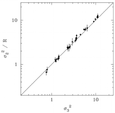
Figure 1: Plot of the estimated 3D density variance, $\sigma_{2}^{2}/R$, versus the actual 3D density variance, $\sigma_{3}^{2}$, obtained from numerical simulations of hydrodynamic turbulence. Each plotted point represents the mean value of $\sigma_{2}^{2}/R$ obtained from analysis of column density fields projected along the three cardinal directions, while the error bars represent the standard deviation in the values of $\sigma_{2}^{2}/R$ for the three directions.

There is a rather more straightforward method of estimating the line-of-sight velocity dispersion, $\sigma_{v_{z}}$, which is simply to measure the dispersion of the mean line profile obtained through imaging observations of an optically-thin spectral line. (This is also a density-weighted measure, however.) If we have an estimate of the cloud temperature, and an estimate of the mean molecular weight, we can then derive the Mach number to construct the right-hand-side of equation (1).

3 Application to Numerical Simulations

As an initial test of the method, we now apply it to numerical simulations of hydrodynamic and magnetohydrodynamic turbulence. Given that the above theory is derived assuming isotropic fields, we investigate the effect of anisotropy using magnetohydrodynamic simulations. In all the studies below, we use normalised column densities ($N/N_{0}$) and normalised densities ($\rho/\rho_{0}$) so that $\sigma_{2}^{2}=\sigma_{N/N_{0}}^{2}$ and $\sigma_{3}^{2}=\sigma_{\rho/\rho_{0}}^{2}$.

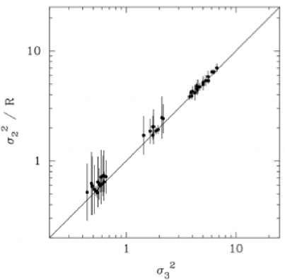
Figure 2: Plot of the estimated 3D density variance, $\sigma_{2}^{2}/R$, versus the actual 3D density variance, $\sigma_{3}^{2}$, obtained from numerical simulations of magnetohydrodynamic turbulence. Each plotted point represents the mean value of $\sigma_{2}^{2}/R$ obtained from analysis of column density fields projected along the three cardinal directions, while the error bars represent the standard deviation in the values of $\sigma_{2}^{2}/R$ for the three directions. The solid line is the line of equality.

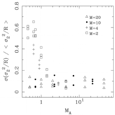
Figure 3: Plot of the standard deviation in $\sigma_{2}^{2}/R$ expressed as a fraction of the mean $\sigma_{2}^{2}/R$, versus the Alfvénic Mach number, $M_{A}$, for the MHD simulations.

3.1 Hydrodynamic Turbulence

First, we analyse hydrodynamic simulations at a range of rms Mach numbers: 1.25, 2.5, 3.5, 5, 7, 10, and 20. Multiple snapshots are used at each Mach number setting, separated by at least a crossing time. The hydrodynamic simulations were run with the phantom Smoothed Particle Hydrodynamics code, with turbulence driven artificially over  5 crossing times using large-scale solenoidal Fourier driving (Price & Federrath 2009; Federrath et al 2009; Brunt, Heyer, & Mac Low 2009; Brunt 2003). For the analysis in this paper we performed a suite of low resolution $128^{3}$ particle calculations, interpolated to $256^{3}$ grids. Since the key idea here is the reconstruction of the density variance, we find that even low resolution calculations are sufficient as demonstrators of the method. For each simulation, we take the 3D density field, of mean unity, and create three normalised projected fields by averaging along each spatial axis. We compute $\sigma_{3}^{2}$ in 3D and a value of $\sigma_{2}^{2}$ for each projected 2D field.

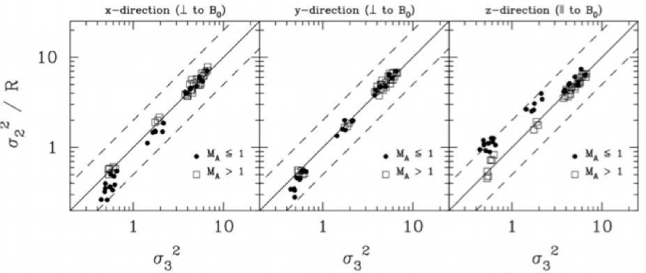
Figure 4: Relations between $\sigma_{2}^{2}/R$ and the true $\sigma^{2}_{3}$ for each of the three axes. Runs with $M_{A}\leq 1$ are shown as dots; runs with $M_{A}>1$ are shown as open squares. The solid line is the line of equality and the dotted lines mark underestimation and overestimation of $\sigma^{2}_{3}$ by a factor of 2.

The power spectrum for each column density field is then measured (specifically, we compute the average power in bins of unit width in $k$.) Following this, equation (26) is used to compute a value of $R$ for each projected field. To do this, we interpolate the binned column density power spectrum to the appropriate power for each $k$ resulting from the nested sums. An extrapolation is required (using a power law fit to the power spectrum in the high $k$ region) for $\sqrt{2}\lambda/2<k\leq\sqrt{3}\lambda/2$ in the denominator. In the above procedure, we emphasize that only information present in the column density field is used in the calculation of $R$. Values of $R$ computed for these fields vary between about 0.03 and 0.15. Note that in general, $R$ will depend on the form of the power spectrum and the scale ratio of the field.

In figure 1 we plot the estimated 3D density variance, $\sigma_{2}^{2}/R$, versus the actual 3D density variance, $\sigma_{3}^{2}$. For each snapshot, we represent the measurements as a mean (plotted point) and standard deviation (error bar) obtained from the three different projections. The method can predict the 3D density variance to about 10% accuracy.

3.2 Magnetohydrodynamic Turbulence

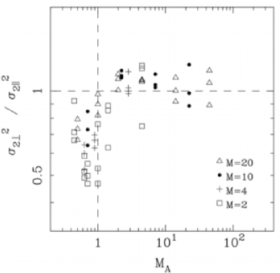
Figure 5: Plot of the anisotropy indicator, $\sigma^{2}_{2\perp}/\sigma^{2}_{2||}$, versus the Alfvénic Mach number, $M_{A}$, for the MHD simulations. For reference, the horizontal dashed line marks the expected value of $\sigma^{2}_{2\perp}/\sigma^{2}_{2||}$ for an isotropic field; the vertical dashed line marks $M_{A}=1$, below which anisotropy is notable.

We now analyse magnetohydrodynamic (MHD) simulations of turbulence. The MHD simulations were run with the grid-based code flash (Fryxell et al. 2000). We used a new approximate Riemann solver for ideal-MHD (Bouchut, Klingenberg, & Waagan 2007, 2009), which preserves positive states in highly supersonic MHD turbulence. This solver was recently developed for flash by Waagan (2009). The corresponding scheme for preserving positive states in hydrodynamical studies has been successfully tested and applied in Klingenberg, Schmidt & Waagan (2007). We used the same solenoidal forcing scheme as used in Federrath et al. (2009) and Price & Federrath (2009). All MHD models were evolved on a fixed grid with $256^{3}$ grid zones.

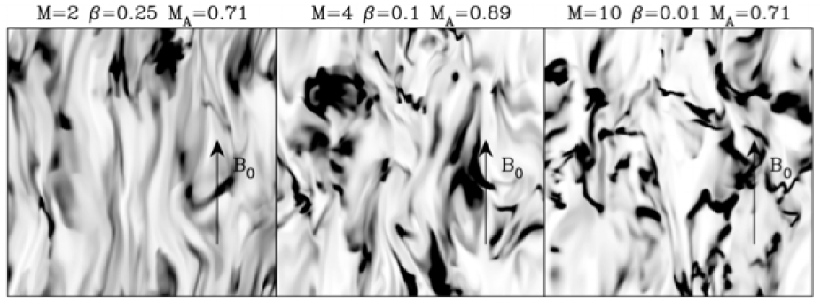
Figure 6: Representative 2D slices through a sample of density fields created by sub-Alfvénic turbulence. The mean magnetic field direction is illustrated by an arrow, labelled $B_{0}$. The values of the sonic Mach number, $M$, the plasma beta, $\beta$, and the Alfvénic Mach number, $M_{A}$ are given above each panel.

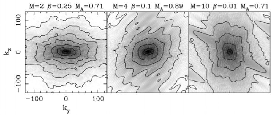
Figure 7: Power spectra of the 2D density field slices from Figure 6. Greyscales are represented in logarithmic units, with contours, each separated by a decade in power, overlayed; the contours been smoothed for clarity.

In addition to varying the Mach number, in the MHD simulations we now also vary the ratio of thermal to magnetic pressure, $\beta=P/(\frac{B_{0}^{2}}{2\mu_{0}})$. For large magnetic field strengths (lower $\beta$) significant anisotropy can arise in the density and velocity fields (Mac Low 1999; Vestuto, Ostriker, & Stone 2003; Heyer et al. 2008), and thus the assumptions of our method could break down. Using the MHD density fields, we repeat the same procedure described above to calculate $R$, and hence the estimated 3D variance, $\sigma^{2}_{2}/R$; the comparison of estimated to true 3D variance is shown in Figure 2. We find that the method is still accurate in predicting the mean (plotted points) but the variation between the different directions (error bars) is now significantly larger for some parameterizations. Investigation of this shows that significant variations in $\sigma^{2}_{2}/R$ between the different projection axes are seen if the Alfvénic Mach number, $M_{A}=M\sqrt{(\beta/2)}$, is smaller than $\sim$ unity. To show this, in Figure 3 we plot the fractional error in the estimated 3D density variance (i.e the standard deviation in $\sigma_{2}^{2}/R$ divided by the mean $\sigma_{2}^{2}/R$ obtained from the three different projection directions) versus $M_{A}$. The fractional error in the estimated 3D density variance is around 10% for $M_{A}>1$, while it increases significantly for $M_{A}<1$.

As there is now notable variation in $\sigma_{2}^{2}/R$ between the different directions, it is worth plotting the individual $\sigma_{2}^{2}/R$ versus $\sigma^{2}_{3}$ relations obtained from each axis. These relations are shown in Figure 4, where we have distinguished the plotted points with different symbols for $M_{A}\leq 1$ and $M_{A}>1$. The 3D variance in sub-Alfvénic runs is overestimated (underestimated) from 2D fields produced by averaging over an axis parallel (perpendicular) to the mean magnetic field direction, by as much as a factor of $\sim$ 2.

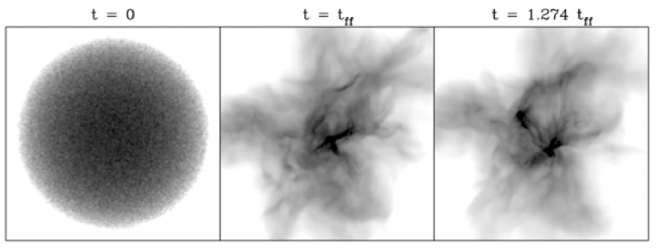
Figure 8: Column density plots (logarithmic greyscale) of the non-periodic SPH simulation.

The variations in $\sigma_{2}^{2}/R$ are caused by anisotropic structure in the density field that is produced when $M_{A}<1$. As a simple measure of this anisotropy, we define an “anisotropy indicator” using the 2D fields that are produced by averaging over the three cardinal axes. The anisotropy indicator is defined as $\sigma^{2}_{2\perp}/\sigma^{2}_{2||}=(\sigma^{2}_{2x}+\sigma^{2}_{2y})/2\sigma^{2}_{2z}$, where $\sigma^{2}_{2x}$, $\sigma^{2}_{2y}$, and $\sigma^{2}_{2z}$ are the variances in the 2D fields produced by averaging over the $x$, $y$, and $z$ axes respectively. The measured values of $\sigma^{2}_{2\perp}/\sigma^{2}_{2||}$ are plotted in Figure 5 versus $M_{A}$. For $M_{A}>1$, $\sigma^{2}_{2\perp}/\sigma^{2}_{2||}$ is $\sim$ unity, indicating roughly equal variances in each of the projected 2D fields. For $M_{A}<1$ the variance in the 2D field averaged over the $z$ direction (parallel to the mean $B$ field) is larger, by as much as a factor of 2, than that of the 2D fields produced by averaging over the $x$ or $y$ directions (perpendicular to the mean $B$ field).

Interestingly, the degree of anisotropy appears to be related to the sonic Mach number, $M$, as is evident in both Figure 3 and Figure 5. Indeed, for $M\geq 10$, the estimation of the 3D variance is not noticeably worse for sub-Alfvénic turbulence than for super-Alfvénic turbulence, and the largest deviations from isotropic behaviour are found in the $M=2$ runs. A direct visualization of the anisotropies present in the density fields is given in Figure 6, which shows representative 2D slices through a sample of density fields produced by sub-Alfvénic turbulence. At low sonic Mach number ($M=2$) the density field is characterized by many long filamentary structures oriented parallel to the mean magnetic field direction. As the sonic Mach number is increased, this directional order in the density field is systematically reduced, until at $M=10$ it is barely noticeable. The power spectra of these 2D density field slices are shown in Figure 7. These confirm our visual assessment of the density field slices. The high frequency spectral power along the magnetic field axis is notably lower in the low sonic Mach number calculations.

The tests on the MHD simulations provide a valuable baseline for establishing the physical regimes in which our method can be applied. In most circumstances encountered in molecular clouds with sizes of a few parsecs, sonic Mach numbers are large enough to enforce sufficient isotropy that the method can work with around 10% accuracy, even for sub-Alfvénic turbulence. However, these are rather idealized conditions, as the models do not include other relevant physics such as self-gravity. Gravitational collapse in the presence of a magnetic field is likely to be oriented along the magnetic field lines if the field is sufficiently strong. Note that the combination of magnetic fields and gravity, in this instance, can induce anisotropic structure in the orthogonal direction to that seen in the sub-Alfvénic simulations described above.

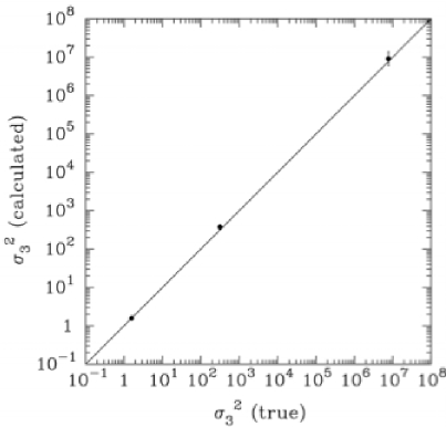
Figure 9: Comparison of calculated to true 3D variances for the non-periodic SPH density fields.

3.3 Non-Periodic Fields

In the foregoing analysis, we have used periodic fields for which there are no edge discontinuities and consequently no zero-padding is required. A more physically realistic scenario is provided by SPH simulations that do not employ periodic boundary conditions. For our analysis, we take density fields produced by the hydrodynamic simulations of Price & Bate (2009). Column density fields extracted at three different times (at $t=0$; after one free fall time; and at the end of the calculation where $t$ = 1.274 $t_{ff}$) are shown in Figure 8. (The column density fields are represented as logarithmic greyscales as the variances are extremely large.) We zero-pad these fields to $\lambda_{p}=512$ from the original $\lambda=256$, then compute the power spectra and from this derive $R_{p}$. We then calculate the 3D variance by use of equation (29).

In Figure 9 we compare the 3D variances derived from our method with the actual 3D variances measured directly from the density fields. We find that the method is comparably accurate for these non-periodic fields, albeit with a rather large variation ($\sim$ 40%) between different projections in the latest snapshot. In this field, the variance is very large indeed ($7.7\times 10^{6}$) and is dominated by a small number of very large density values caused by localised gravitational collapse. The variances in the initial density field (a spherical blob), in the $t=t_{ff}$ density field, and in the $t=1.274~{}t_{ff}$ density field are recovered by the mean calculated variances to within 0.3%, 20% and 20% accuracy respectively. To evaluate the success of these measurements, we calculate an anisotropy indicator as was done in Section 3.2, by taking the ratio of the variance in one projected field to the mean of the variances in the other two projected fields. Since the simulations contain no magnetic fields, there is no preferred axis. Therefore we combine the three 2D variance measurements in a way that minimises the anisotropy indicator (lower values represent greater degrees of anisotropy). For the three snapshots, in increasing-time-order, we find anisotropy indicators of 1.00, 0.78, and 0.54. For the two evolved snapshots, the density fields are comparably anisotropic to the low $M_{A}$, low $M$ density fields of the previous section, but with the anisotropy now arising from the initial velocity perturbations rather than from the effect of a magnetic field. The accuracy of the method for non-periodic boundary conditions is therefore comparable to the periodic case when compared at the same level of intrinsic anisotropy.

The extremely high variances seen in the evolved density fields are a result of small-scale collapse in this gravitationally-bound cloud, and far exceed variances expected by equation (1) with $b\approx 0.5$. It will be interesting in future to see how equation (1) is modified in strongly-self-gravitating clouds, and whether observations can quantify this.

4 Conclusions

We have introduced and tested a simple method for measuring the 3D density variance in molecular clouds, using only information present in the projected column density field. The method relies on the assumption of isotropy and uses the measured column density power spectrum in conjunction with Parseval’s theorem to calculate a correction factor, $R$, that scales the observed normalised column density variance to the intrinsic three-dimensional normalised density variance. The method is sufficiently general to be applied to any isotropic field.

For density fields produced in supersonic hydrodynamic and magnetohydrodynamic turbulence, the method is accurate to about 10% provided that the assumption of isotropy is valid. For turbulent density fields, in practice this requires that the turbulence motions are super-Alfvénic ($M_{A}<1$), though even in the sub-Alfvénic regime we are able to recover the 3D variance for high sonic Mach number ($M\gtrsim 10$).

References

- Bensch, Stutzki, & Ossenkopf (2001) Bensch, F., Stutzki, J., & Ossenkopf, V., 2001, A&A, 366, 636
- Bouchut et al. (2007) Bouchut, F., Klingenberg, C., & Waagan, K. 2007, Numerische Mathematik, 108, 7
- Bouchut et al. (2009) Bouchut, F., Klingenberg, C., & Waagan, K. 2009, Numerische Mathematik, accepted
- Brunt (2009) Brunt, C. M., 2009, submitted to A&A
- Brunt (2003) Brunt, C. M., 2003, ApJ, 583, 280
- Brunt, Heyer, & Mac Low (2009) Brunt, C. M., Heyer, M. H., & Mac Low, 2009, A&A, 504, 883
- Brunt & Mac Low (2004) Brunt, C. M., & Mac Low, 2004, ApJ, 604, 196
- Elmegreen (2008) Elmegreen, B. G., 2008, ApJ, 672, 1006
- Federrath, Klessen, & Schmidt (2008) Federrath, C., Klessen, R. S., & Schmidt, W., 2008, ApJ, 688, 79
- Federrath et al (2009) Federrath, C., Duval, J., Klessen, R., Schmidt, W., & Mac Low, M.-M., 2009, arXiv, 0905.1060
- Fryxell et al (2000) Fryxell, B., Olson, K., Ricker, P., Timmes, F. X., Zingale, M., Lamb, D. Q., MacNiece, P., Rosner, R., Truran, J. W., & Tufo, H., 2000, ApJS, 131, 273
- Goodman, Pineda, & Schnee (2009) Goodman, A. A., Pineda, J. E., & Schnee, S. L., 2009, ApJ, 692, 91
- Hartmann (2002) Hartmann, L., 2002, ApJ, 578, 914
- Hennebelle & Chabrier (2008) Hennebelle, P., & Chabrier, G., 2008, ApJ, 684, 395
- Hennebelle & Chabrier (2009) Hennebelle, P., & Chabrier, G., 2009, ApJ, 702, 1428
- Heyer et al (2008) Heyer, M. H., Gong, H., Ostriker, E., & Brunt, C., 2008, ApJ, 680, 420
- Klingberg, Schmidt, & Waagan (2007) Klingberg, C., Schmidt, W., & Waagan, K., 2007, J. Comp. Phys., 227, 12
- Krumholz & McKee (2005) Krumholz, M. R., & McKee, C. F., 2005, ApJ, 630, 250
- Lazarian & Pogosyan (2000) Lazarian, A., & Pogosyan, D., 2000, ApJ, 537, 720
- Lucy (1974) Lucy, L. B., 1974, AJ, 79, 745
- Mac Low (1999) Mac Low, M.-M., 1999, ApJ, 524, 169
- Miville-Deschenes & Martin (2007) Miville-Deschenes, M.-A., & Martin, P. G., 2007, A&A, 469, 189
- Ostriker, Stone, & Gammie (2001) Ostriker, E. C., Stone. J. M., & Gammie, C. F., 2001, ApJ, 546, 980
- Padoan, Nordlund, & Jones (1997) Padoan, P., Nordlund, Å., & Jones, B. J. T., 1997, MNRAS, 288, 145
- Padoan & Nordlund (2002) Padoan, P., & Nordlund, Å., 2002, ApJ, 576, 870
- Padoan & Nordlund (2009) Padoan, P., & Nordlund, Å., 2009, arXiv, 0907.0248
- Passot & Vázquez-Semadeni (1998) Passot, T., & Vázquez-Semadeni, E., 1998, PhRvE, 58, 4501
- Price & Bate (2009) Price, D. J., & Bate, M. R., 2009, MNRAS, 398, 33
- Price & Federrath (2009) Price, D. J., & Federrath, C., 2009, submitted to MNRAS
- Reblinsky (2000) Reblinsky, K., 2000, A&A, 364, 377
- Stutzki et al (1998) Stutzki, J., Bensch, F., Heithausen, A., Ossenkopf, V., & Zeilinsky, M., 1998, A&A, 336, 697
- Vázquez-Semadeni (1994) Vázquez-Semadeni, E., 1994, ApJ, 423, 681
- Vázquez-Semadeni, Ballesteros-Paredes, & Klessen (2003) Vázquez-Semadeni, E., Ballesteros-Paredes, J., & Klessen, R. S., 2003, ApJ, 585, L131
- Vázquez-Semadeni & García (2001) Vázquez-Semadeni, E., & García, N., 2001, ApJ, 557, 727
- Vestuto, Ostriker, & Stone (2003) Vestuto, J. G., Ostriker, E. C., & Stone, J. M., 2003, ApJ, 590, 858
- Waagan (2009) Waagan, K. 2009, Journal of Computational Physics, 228, 860