Dynamical transitions and sliding friction of the phase-field-crystal model with pinning

Abstract

We study the nonlinear driven response and sliding friction behavior of the phase-field-crystal (PFC) model with pinning including both thermal fluctuations and inertial effects. The model provides a continuous description of adsorbed layers on a substrate under the action of an external driving force at finite temperatures, allowing for both elastic and plastic deformations. We derive general stochastic dynamical equations for the particle and momentum densities including both thermal fluctuations and inertial effects. The resulting coupled equations for the PFC model are studied numerically. At sufficiently low temperatures we find that the velocity response of an initially pinned commensurate layer shows hysteresis with dynamical melting and freezing transitions for increasing and decreasing applied forces at different critical values. The main features of the nonlinear response in the PFC model are similar to the results obtained previously with molecular dynamics simulations of particle models for adsorbed layers.

I Introduction

In recent years, considerable attention has been given to the study of driven adsorbed layers in relation to sliding friction phenomena between surfaces at the microscopic level Israelechvili ; Book ; Conf ; Persson93 ; Granato99 ; Granato00 . The nonlinear response of the adsorbed layer is a central problem for understanding experiments on sliding friction between two surfaces with a lubricant Israelechvili or between adsorbed layers and an oscillating substrate Krim ; Mistura . Various elastic and particle models have been used to study the driven dynamical transitions and the sliding friction of adsorbed monolayers Persson93 ; Book ; Conf ; Granato99 . A fundamental issue in modeling such systems is the origin of the hysteresis and the dynamical melting and freezing transitions associated with the different static and kinetic frictional forces when increasing the driving force from zero and decreasing from a large value, respectively. In driven lattice systems, hysteresis can occur in the underdamped regime where inertial effects are present or in the presence of topological defects such as dislocations and thermal fluctuations Fisher85 . Topological defects can be automatically included in a full microscopic model involving interacting atoms in the presence of a substrate potential using realistic interaction potentials. However, numerical observation of the full complexities of the phenomena is severely limited by the small system sizes that can be studied, even when simple Lennard-Jones potentials are employed Persson93 .

Recently, a phase-field-crystal (PFC) model was introduced Elder02 ; Elder04 ; Elder07 that allows for both elastic and plastic deformations within a continuous description of the particle density while still retaining information on atomic length scales. By extending the PFC model to take into account the effect of an external pinning potential achim06 , a two-dimensional version of the model has been used to describe commensurate-incommensurate transitions in the presence of thermal fluctuations ramos08 and the driven response of pinned lattice systems without thermal fluctuations and inertial effects. achim09 . However, in order to study fully the sliding friction behavior, both inertial effects and thermal fluctuations need to be taken into account.

In this work, we study sliding friction of an adsorbed layer via the nonlinear response of the PFC model to an external force in the presence of a pinning potential. To this end, we first derive the general stochastic dynamical equations for the particle and momentum density fields taking full account of the thermal fluctuations and inertial effects. The resulting coupled equations are studied numerically. At low temperatures, we find that the velocity response of an initially commensurate layer shows hysteresis with dynamical melting and freezing transitions for increasing and decreasing applied forces at different critical values. The main features of the nonlinear response are similar to the results obtained previously with molecular dynamics simulations of particle models. However, the dynamical melting and freezing mechanisms are significantly different. In the PFC model, nucleation occurs via stripes rather than closed domains found in the particles model.

II Dynamics of the PFC model with inertial effects

In the generalized PFC model, the system is represented by a coarse grained effective Hamiltonian that is a functional of the number density field. To take into account inertial effects in the dynamics, we need to consider the contribution of the kinetic energy to the total energy of the system in addition to the configurational energy. Thus we consider the momentum density, $\vec{g}(\vec{x})=\rho(\vec{x})\vec{v}(x)$, a dynamical variable in the coarse grained Hamiltonian in addition to the particle density field $\rho(\vec{x})$. The total effective Hamiltonian in the presence of an external force $\vec{f}$ can be written as

$$H_{t}=H_{kin}+H_{int}-\int d\vec{x}\rho(\vec{x})\vec{x}\cdot\vec{f},$$ (1)

where $H_{kin}$ is the kinetic energy contribution given by

$$H_{kin}=\int d\vec{x}\frac{{\vec{g}}^{2}(\vec{x})}{2\rho(\vec{x})},$$ (2)

and $H_{int}(\rho)$ is the configurational contribution to the effective Hamiltonian in the original PFC model. The last term is due to the presence of the the external force $\vec{f}$.

In the absence of energy dissipation, the time dependence of $\rho$ and $\vec{g}$ are determined by the Poisson brackets $\{H_{t},\rho\}$ and $\{H_{t},\vec{g}\}$. At finite temperatures, additional dissipative noise terms are present in the dynamical equations. The noise satisfies the fluctuation dissipation relations chaikin ; mazenkob which allows the system to reach thermal equilibrium in the absence of external perturbations. We include the dissipative noise term directly in the dynamical equations for $\vec{g}$, which is a nonconserved field.

For the particle density $\rho(\vec{x},t)$ we have

$$\frac{\partial\rho}{\partial t}=-\sum_{j}\int d{\vec{x}}^{\prime}\{\rho(\vec{x}),g_{j}(\vec{x}^{\prime})\}\frac{\delta H_{t}}{\delta g_{j}(\vec{x}^{\prime})},$$ (3)

and for the momentum density $\vec{g}(x,t)$

$$\frac{\partial g_{i}}{\partial t} = -\int d{\vec{x}}^{\prime}\{g_{i}(\vec{x}),\rho(\vec{x}^{\prime})\}\frac{\delta H_{t}}{\delta\rho(\vec{x}^{\prime})}$$ (6)

$$-\sum_{j}\int d{\vec{x}}^{\prime}\{g_{i}(\vec{x}),g_{j}(\vec{x}^{\prime})\}\frac{\delta H_{t}}{\delta g_{j}(\vec{x}^{\prime})}$$

$$-\eta\frac{\delta H_{t}}{\delta g_{i}}+\nu_{i}(\vec{x},t),$$

where $\eta$ is a dissipative coefficient and the noise $\vec{\nu}(\vec{x},t)$ has variance

$$\langle\nu_{i}(\vec{x},t)\nu_{j}(\vec{x}^{\prime},t^{\prime})\rangle=2k_{B}T\eta\delta(\vec{x}-\vec{x}^{\prime})\delta(t-t^{\prime})\delta_{i,j}.$$ (7)

The Poisson brackets for the mass and momentum densities are given by chaikin ; mazenkob

$$\{\rho(\vec{x}),g_{i}(\vec{x}^{\prime})\} = \nabla_{i}(\rho(\vec{x})\delta(\vec{x}-\vec{x}^{\prime}));$$ (8)

$$\{g_{i}(\vec{x}),\rho(\vec{x}^{\prime})\} = \rho(\vec{x})\nabla_{i}\delta(\vec{x}-\vec{x}^{\prime});$$

$$\{g_{i}(\vec{x}),g_{j}(\vec{x}^{\prime})\} = \nabla_{j}(g_{i}(\vec{x})\delta(\vec{x}-\vec{x}^{\prime}))-\nabla_{i}^{\prime}(g_{j}(\vec{x})\delta(\vec{x}-\vec{x}^{\prime})).$$

Substituting Eqs. (8) into Eqs. (3) and (6) gives

$$\frac{\partial\rho}{\partial t}=-\nabla\cdot\vec{g};$$ (9)

$$\frac{\partial g_{i}}{\partial t}=-\rho\nabla_{i}\frac{\delta H_{int}}{\delta\rho} - \eta\frac{g_{i}}{\rho}+\rho f_{i}+\nu_{i}(\vec{x},t)$$

$$-\sum_{j}\nabla_{j}\frac{g_{i}g_{j}}{\rho},$$

for a spatially uniform external force ($f_{i}$). We can redefine the coefficient $\eta\rightarrow\rho\eta$ to remove the denominator from the term $g_{i}/\rho$ in Eq. (II). With this change the variance of the noise $\vec{\nu}(x,t)$ becomes

$$\langle\nu_{i}(\vec{x},t)\nu_{j}(\vec{x}^{\prime},t^{\prime})\rangle=2k_{B}T\eta\rho(\vec{x})\delta(\vec{x}-\vec{x}^{\prime})\delta(t-t^{\prime})\delta_{i,j}$$ (11)

To leading order in the momentum density $\vec{g}$, we drop the quadratic term in Eq. (II) giving

$$\frac{\partial\rho}{\partial t}=-\nabla\cdot\vec{g};$$ (12)

$$\frac{\partial g_{i}}{\partial t}=-\rho\nabla_{i}\frac{\delta H_{int}}{\delta\rho}+\rho f_{i}-\eta g_{i}+\nu_{i}(\vec{x},t).$$ (13)

Similar dynamical equations for PFC models with internal dissipation were obtained in Ref. sami, . If the effective Hamiltonian $H_{int}$ is known, then these coupled stochastic dynamical equations should provide a full description of the particle and momentum densities in presence of fluctuations represented by the noise $\nu_{i}(x,t)$ with correlations proportional to the temperature $T$ and inertial effects determined by the damping parameter $\eta$. In the overdamped limit, $\partial{g}/\partial{t}=0$, with $T=0$ and $f=0$, the equation for the time evolution of $\rho$ obtained by inserting $\vec{g}$ from Eq. (13) in Eq. (12) reduces to the deterministic equation for the density which has been obtained from classical density functional theory of liquids Voigt .

III PFC model with pinning and thermal fluctuations

In the presence of an external pinning potential achim06 ; ramos08 ; achim09 , a specific form of the configurational energy contribution $H_{int}$ to the total effective Hamiltonian in Eq.(1) has been proposed which is an extension of the standard PFC model free energy functional used in many applications Elder04 ; Elder07 . In dimensionless form, this effective interaction Hamiltonian $H_{int}=H_{\rm pfc}$ can be written as

$$H_{\rm pfc}=\int d\vec{x}\{\frac{1}{2}\psi[r+(1+\nabla^{2})^{2}]\psi+\frac{\psi^{4}}{4}+V\psi\},$$ (14)

where $\psi(\vec{x})$ is a continuous field, $V(\vec{x})$ represents the external pinning potential and $r$ is a parameter. The phase field $\psi(\vec{x})$ can be regarded as a measure of deviations of the particle number density $\rho(\vec{x})$ from a uniform reference value $\rho_{0}$, such that $\psi(\vec{x})=(\rho(\vec{x})-\rho_{0})/\rho_{0}$. It is a conserved field and its average value, $\bar{\psi}$, represents another parameter in the model. The intrinsic wave vector of the model $\vec{k}_{i}$ has no preferred directions and its magnitude is set to unity in the present work.

In the absence of a pinning potential, the Hamiltonian of Eq. (14) is minimized by a configuration of the field $\psi(\vec{x})$ forming a hexagonal pattern of peaks with reciprocal lattice vectors of magnitude $|\vec{k}_{h}|\approx 1$, in an appropriate range of values for the parameters $r$ and $\bar{\psi}$ in the model. This periodic structures of peaks in $\psi$ can be regarded as a simple model of an atomic layer.

To study the nonlinear dynamical behavior we take the form of $H_{int}$ given by Eq.(14) together with the kinetic energy and the external force terms for the total effective Hamiltonian $H_{t}$ in the dynamical equations Eq. (13) and in Eq. (11). We make the additional simplifying approximation that $\rho(\vec{x})\approx\rho_{0}$ in Eq. (11) and in the coefficient of the first term in Eq. (13). This approximation ensures that the effective diffusion coefficient in the model is positive definite for any temperature and driving force. Another motivation for this approximation is to show that the dynamical equations used in the previous works achim06 ; achim09 follows from the more general Eqs. (12) and (13). Setting $\rho_{0}=1$, we obtain,

$$\frac{\partial\psi}{\partial t}=-\nabla\cdot\vec{g};$$ (15)

$$\frac{\partial g_{i}}{\partial t}=-\nabla_{i}\frac{\delta H_{pfc}}{\delta\psi} + \psi f_{i}-\eta g_{i}+\nu_{i}(\vec{x},t);$$

$$\langle\nu_{i}(\vec{x},t)\nu_{j}(\vec{x}^{\prime},t^{\prime})\rangle = 2k_{B}T\eta\delta(\vec{x}-\vec{x}^{\prime})\delta(t-t^{\prime})\delta_{i,j}.$$

Here we have redefined $\vec{g}\rightarrow\vec{g}+\rho_{0}\vec{f}/\eta$ to remove a uniform term on right hand side of the equation for $\vec{g}$.

The above coupled equations can be combined in a single equation by applying the operator $\nabla\cdot$ to both sides of the second equation and using the first one to eliminate $\nabla\cdot\vec{g}$, giving

$$\frac{\partial^{2}\psi}{\partial t^{2}}+\eta\frac{\partial\psi}{\partial t} = \nabla^{2}\frac{\delta H_{\rm pfc}}{\delta\psi}-\vec{f}\cdot\nabla\psi+\xi(\vec{x},t);$$ (16)

$$\langle\xi(\vec{x},t)\xi(\vec{x}^{\prime},t^{\prime})\rangle = 2k_{B}T\eta\nabla^{2}\delta(\vec{x}-\vec{x}^{\prime})\delta(t-t^{\prime}).$$

When the driving force $\vec{f}$ and the external pinning potential are set to zero, the dynamical equation above is identical to the one used in Ref. stefano, to study propagating density modes in the PFC model. It can also be obtained by introducing inertial effects in the dynamical equation of the PFC model through a memory function of exponential formGalenko . In the limit of large $\eta$ when $\partial g_{i}/\partial t$ in Eqs. (15) or, equivalently, $\partial^{2}\psi/\partial t^{2}$ in Eqs. (16), can be neglected, these equations reduce to the familiar overdamped dynamical equations used in the previous works achim06 ; achim09 without inertial effects at zero temperature.

IV Numerical results and Discussion

In this section, we present our numerical results for the velocity response of the PFC model in presence of an external pinning potential under a uniform applied force. For the numerical calculations, the phase field $\psi(\vec{x})$ and momentum density field $\vec{g}(\vec{x})$ are defined on a space square grid with $dx=dy=\pi/4$ with periodic boundary conditions. System sizes $L\times L$ with $L=64$ to $128$ where used. The Laplacians and gradients were evaluated using finite differences.

We consider a pinning potential $V(\vec{x})$ representing a substrate with square symmetry

$$V(\vec{x})=-V_{0}[\cos(k_{0}x)+\cos(k_{0}y)],$$ (17)

where $k_{0}$ defines the period of the pinning potential for both the $x$ and $y$ directions. The lattice misfit between the phase-field crystal and the pinning potential can be defined as $\delta_{\rm m}=(1-k_{0})$. We choose the parameters of the PFC model as $r=-0.25$, $\bar{\psi}=-0.25$, a lattice mismatch $\delta=-0.5$ and a pinning strength $V_{0}=0.15$. For these parameters, the ground-state configuration in the absence of an external driving force is a $c(2\times 2)$ phase ramos08 ; achim09 , where every second site of the lattice of the pinning potential corresponds to a peak in the phase field $\psi(\vec{r})$. This commensurate configuration is stable below a commensurate melting temperature $T_{c}\approx 0.055$. This is determined from the temperature dependence of the structure factor as well as that of the specific heat. The structure factor $S(\vec{k})$ is calculated from the the positions $\vec{R}_{j}$ of the peaks in the phase field as

$$S(\vec{k})=\langle\sum_{j,j^{\prime}=1}^{N_{P}}\frac{1}{N_{P}}e^{-i\vec{k}\cdot(\vec{R}_{j}-\vec{R}_{j^{\prime}})}\rangle.$$ (18)

Here, $\langle...\rangle$ denotes a time average which is equivalent to a thermal average at equilibrium. For increasing temperatures thermal fluctuations disorder the layer and the scaled structure factor $S(\vec{k}_{c})/N_{p}$ evaluated at the primary reciprocal lattice vector $\vec{k}_{c}$ of the commensurate phase decreases from a value of unity at $T=0$ rapidly through $T_{c}$ to zero at higher temperatures. The transition is broadened due to finite size effects as shown in Fig. 1(a). Another signature of this commensurate melting transition is that the specific heat develops a broad peak near $T_{c}$ corresponding to an increase in the fluctuations in $\psi$ at the transition as shown in Fig. 1(b). Finally, the mobility $\mu$ defined as $\lim_{f\to 0}(v/f)$ where $v$ is the drift velocity, also changes qualitatively through the transition. In the commensurate phase, a finite threshold for the sliding of the overlayer exists and hence the mobility is vanishingly small. As the system melts above $T_{c}$ the mobility rapidly rises and reaches a plateau at higher temperatures. This behavior is shown in Fig. 1c. For the study of the nonlinear response and sliding friction of the system, we focus on an initial state which corresponds to a well pinned $c(2\times 2)$ phase initially, corresponding to $T=0.01\ll T_{c}$, and a damping parameter $\eta=0.4$.

In our numerical calculations, a driving force along the $x$ direction is increased from zero to a maximum value above a critical depinning force and then decreased back to zero. For each value of the force, the coupled equations (15) are solved using an Euler algorithm with time step $dt=0.001-0.005$. The implicit trapezoidal method was also used to check numerical stability. For each value of the force, $10^{6}$ time steps were used to allow the system to reach a velocity steady state and an additional period with the same number of time steps were used to calculate the average velocity and other time averaged quantities.

To study the velocity response of the PFC model, we need to determine the velocity of the peaks ramos08 in the phase field $\psi(\vec{x})$. This is done by determining the time dependence of the peak positions ($\vec{R}_{i}(t)$) in $\psi$. The steady state drift velocity $\vec{v}$ for the system is obtained from the peak velocities $\vec{v}_{i}$ ($d\vec{R}_{i}/dt$) as

$$\vec{v}=\langle\frac{1}{N_{P}}\sum_{i=1}^{N_{P}}\vec{v}_{i}(t)\rangle,$$ (19)

where $N_{P}$ is the number of peaks and $\langle...\rangle$ denotes time average. The steady state structure factor $S(\vec{k})$ which is a measure of translational order, is also calculated from the the peak positions $\vec{R}_{j}$, as in Eq.(18).

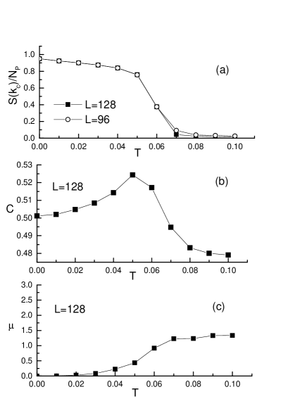
Figure 1: Temperature dependence of the (a) scaled structure-factor peak $S(k_{c})/N_{p}$; (b) specific heat $C$, and mobility $\mu$ for the model without an external driving force.

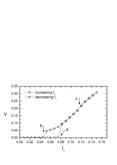
Figure 2: Velocity response as a function of applied force. Arrows correspond to critical values $f_{a}$, $f_{b}$ and $f_{c}$.

The most notable qualitative feature of the velocity response to the driving force $\vec{f}$ (as shown in Fig. 2) is that it shows hysteresis behavior with two different critical force thresholds $f_{a}\approx 0.075$ for increasing forces and $f_{b}\approx 0.045$ for decreasing forces. These two threshold values correspond to the static frictional force and kinetic frictional force respectively. As the force is increased beyond $f_{a}$, the velocity jumps abruptly from zero to a finite value whereas when the force is decreased below $f_{b}$ the velocity of the sliding layer drops abruptly and become pinned by the external potential to form an immobile commensurate state again. Below, we present the microscopic details of the configurations for the system in the neighborhood of the two thresholds. This allows us to characterize the change in velocity response at $f_{a}$ as a dynamical force induced melting transition of the initial commensurate state, and the second transition at $f_{b}$ as a dynamical force induced freezing of the sliding phase.

To study these transitions we first examine the behavior of the steady state structure factor, as shown in Fig. 3. We focus on the dependence of $S(Q)$ on the driving force, where $\vec{Q}$ is the dominant reciprocal lattice vector of the layer. $\vec{Q}=\vec{k}_{c}$ corresponds to the primary reciprocal lattice vector for the $c(2\times 2)$ phase and $\vec{Q}=\vec{k}_{h}$ to the reciprocal lattice vector of the hexagonal phase in absence of the driving force. Consistent with the velocity response behavior in Fig. 2, on increasing the force beyond $f_{a}$, $S(k_{c})$ drops abruptly to zero. This is the onset of the dynamical force induced melting transition of the initial $c(2x2)$ commensurate state. The behavior of $S(k_{c})$ is analogous to the temperature induced disordering transition shown in Fig. 1(a). On decreasing the force, the value of $S(k_{c})$ stays vanishingly small until the force drops below the threshold $f_{b}$, at which point $S(k_{c})$ rapidly increases to a value corresponding to the commensurate pinned state. The other interesting feature is that for $f>f_{c}\approx 0.12$, the structure factor shows clear $6$-fold coordinated peaks at the reciprocal lattice vectors $\vec{Q}=\vec{k}_{h}$ corresponding to a hexagonal phase, which grows as the driving force increases. This implies that at a driving force larger than this third threshold $f_{c}$, there is another dynamic continuous transition from a disordered phase into an incommensurate hexagonal phase. This state emerges as the average effect of the external pinning potential becomes less and less important at high sliding velocities and the steady state then approximately corresponds to the phase-field crystal in the absence of the pinning potential which has hexagonal symmetry in the equilibrium state. However, since the scaled structure factor for the hexagonal phase is still much less than unity, this incommensurate hexagonal phase is not fully ordered even at at the largest force values ($f<0.15$) studied so far.

Figure 3: Scaled structure-factor peak $S(Q)/N_{p}$ as a function of applied force. Here $\vec{Q}$ stands for the primary reciprocal lattice vector for either the $c(2\times 2)$ phase ($\vec{k}_{c}$) or the hexagonal phase ($\vec{k}_{h}$). Filled and open symbols correspond to increasing and decreasing forces, respectively.

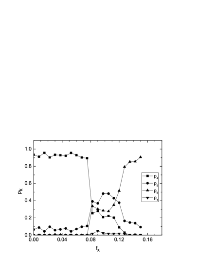
Figure 4: Fraction of density peaks $p_{k}$ with coordination number $k$ (4,5,6 and 7 nearest neighbors) for increasing applied force.

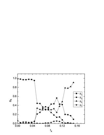
Figure 5: Fraction of density peaks $p_{k}$ with coordination number $k$ for decreasing applied force.

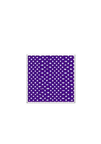
Figure 6: Snapshot of the density field in the sliding state at $f_{x}=0.0525$.

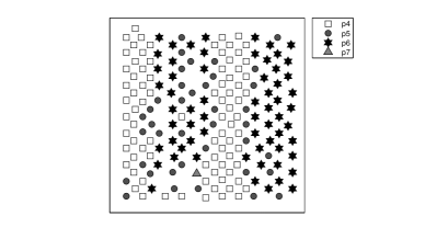
Figure 7: Configuration of the density peak locations with corresponding coordination numbers for the density plot in Fig. 6.

To better understand the dynamic melting transition at $f_{a}$ and the freezing transition at $f_{b}$, we inspect the steady state configurations near the two thresholds as well as the region between the two thresholds in real space, which yield more direct and detailed information than the structure factor at the peak values. Treating the peaks in the phase field as ”particles”, the coordination number of each particle in the commensurate $c(2\times 2)$ phase is $4$ while for the incommensurate hexagonal phase it is $6$. Furthermore, the core of dislocations in a hexagonal lattice correspond to particles with $5$-fold and $7$-fold coordination numbers. Thus, further insight into the microscopic nature of the steady state configurations can be obtained by inspecting the fraction of particles with coordination numbers $p_{4}$, $p_{5}$, $p_{6}$, $p_{7}$. The results are shown in Figs. 4 and Fig. 5 for increasing and decreasing applied forces respectively. Fig. 4 shows that when the force $f$ is increased beyond $f_{a}$, besides the rapid drop in $p_{4}$ consistent with the structure factor data, the fraction of other coordination numbers $p_{5}$, $p_{6}$, $p_{7}$ also increases significantly untill $f$ reaches $f_{c}$, beyond which $p_{5}$ and $p_{7}$ start to decrease and we have a continuous transition to an incommensurate hexagonal phase. Thus the nature of steady state above $f_{a}$ is a strongly disordered state analogous to the high temperature phase in the absence of driving force above the commensurate melting temperature. On decreasing the force below $f_{a}$, the data in Fig. 5 shows that the system remains in a melted state with large disorder until the threshold $f_{b}$ is reached, below which we have only $4$-fold coordination number and the system returns to a pinned $c(2\times 2)$ phase. Taken together, the qualitative behavior of the structure factor and the coordination number strongly suggest that the transitions at $f_{a}$ and $f_{b}$ can be regarded as a force induced dynamical melting and freezing transition respectively.

Finally, we look at a snapshot of the phase field $\psi(x)$ obtained in the steady state for a driving force just above the dynamical freezing threshold $f_{b}$. This is shown in Fig. 6. It consists of stripes of commensurate $c(2\times 2)$ phase separated by disordered domain walls. These domain walls are mobile liquid like regions as confirmed by a count of the fraction of various coordination numbers shown in Fig. 7. The commensurate stripes have only $4$-fold coordination numbers, while in the liquid like domain walls, there is a mixture of $5$-fold, $6$-fold and $7$-fold coordination numbers. Starting from this steady state which still has a non-zero average sliding velocity, we can watch the dynamical freezing in real time as the driving force is reduced to a value just below the freezing threshold $f_{b}$. The time sequence of the freezing is shown in Fig. 8. In returning to the pinned state, the domain wall regions gradually shrink and eventually disappear.

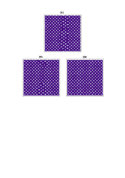
Figure 8: Snapshots of the density field for increasing times after starting from the moving state of Fig. 6 and reaching the pinned commensurate state, at a force $f_{x}=0.045$ just below $f_{b}$. Times are in units of $10^{3}$ time steps.

The main features of the dynamical melting and freezing and hysteresis effects in PFC model described above are similar to those found earlier by molecular dynamics simulations of particle models with interacting Lennard-Jones potentials Persson93 and the uniaxial Frenkel-Kontorova model Granato99 under a driving force starting from a commensurate state. The similarity of results from these very different models demonstrates the universality of the hysteresis loop for models with inertia effects and the macroscopic consequence of stick and slip motion. When compared with the Lennard-Jones particle model one notable difference is the mechanism of the dynamical freezing at $f_{b}$. In the present PFC model, it involves parallel liquid-like domain walls similar to the uniaxial Frenkel-Kontorova model, although in the absence of the driving force there is no easy direction. In the Lennard-Jones model, nucleation and growth occur via closed pinned domains Persson93 . The origin of this intriguing difference requires further investigation of both atomistic and PFC models. One possibility is that the nucleation of stripes is related to the absence of a fixed constraint on the number of peaks in the PFC model. In this case, the mechanism of the dynamical freezing found in the present PFC model should be compared to the results of particle models with a constant chemical potential rather than with a fixed particle number. Unfortunately, such results are currently unavailable.

V Conclusions

In this paper, we have derived general stochastic dynamical equations for the particle and momentum density fields including both thermal fluctuations and inertial effects. The new equations are applied to the study of the nonlinear response to an external driving force for a PFC model with a pinning potential. The model describes a driven adsorbed layer as a continuous density field, allowing for elastic and plastic deformations. The numerical results showed that at low temperatures, the velocity response of an initially commensurate layer shows hysteresis with dynamical melting and freezing transitions for increasing and decreasing applied forces at different critical values. The inclusion of both thermal fluctuations and inertial effects are crucial for a correct description of these dynamical transitions. The main features of the nonlinear response, in particular the hysteresis loop separating the static friction and sliding friction thresholds are similar to the results obtained previously with particle models. However, the details of the dynamical melting and freezing mechanisms are significantly different. In the PFC model considered here, they correspond to nucleation of stripes rather than closed domains found in particle models. It is possible to describe more realistic sliding adsorbed systems if the parameters of the model are adjusted to match experimental systems, similar to the recent works for the colloidal systems Voigt and Fe akusti .

- (1) B.N.J. Persson, Sliding Friction: Physical Principles and Applications (Springer, Heidelberg, 1998).
- (2) articles in Physics of Sliding Friction, edited by B.N. J. Persson and E. Tosatti (Kluwer, Dordrecht,1996).
- (3) B. N. J. Persson, Phys. Rev. Lett. 71, 1212 (1993); J. Chem. Phys. 103, 3449 (1995).
- (4) H. Yoshizawa, P. McGuiggan, and J. Israelachvili, Science 259, 1305 (1993) 14), 109 (1992); Klafter, D. Gourdon, and J. Israelachvili, Nature 430, 525 (2004).
- (5) E. Granato and S. C. Ying, Phys. Rev. B. 59, 5154 (1999).
- (6) E. Granato and S.C. Ying, Phys. Rev. Lett. 85, 5368 (2000); Phys. Rev. B 69, 125403 (2004).
- (7) J. Krim, D.H. Solina, and R. Chiarello, Phys. Rev. Lett. 66, 181 (1991)
- (8) A. Carlin, L. Bruschi, M. Ferrari, and G. Mistura, Phys. Rev. B 68, 045420 (2003).
- (9) D. S. Fisher, Phys. Rev. B 31, 1396 (1985).
- (10) K.R. Elder, M. Katakowski, M. Haataja, and M. Grant, Phys. Rev. Lett. 88, 245701 (2002).
- (11) K.R. Elder, and M. Grant, Phys. Rev. E 70, 051605 (2004).
- (12) K.R. Elder, N. Provatas, J. Berry, P. Stefanovic, and M. Grant, Phys. Rev. B 75, 064107 (2007).
- (13) C.V. Achim, M. Karttunen, K.R. Elder, E. Granato, T. Ala-Nissila, and S.C. Ying, Phys. Rev. E 74, 021104 (2006); J. Phys.: Conf. Ser. 100, 072001 (2008).
- (14) J.A.P. Ramos, E. Granato, C.V. Achim, S.C. Ying, K.R. Elder, T. Ala-Nissila, Phys. Rev. E 78, 031109 (2008).
- (15) C.V. Achim, J.A.P. Ramos, M. Karttunen, K.R. Elder, E. Granato, T. Ala-Nissila, and S.C. Ying, Phys. Rev. E 79, 011606 (2009).
- (16) P.M. Chaikin and T.C. Lubensky, Principles of Condensed Matter Physics, Cambridge University Press, 1995.
- (17) G. Mazenko, Nonequilibrium Statistical Mechanics, Willey-VCH, 2006).
- (18) S. Ramaswamy and G.F. Mazenko, Phys. Rev. A 26, 1735 (1982).
- (19) B.N.J. Persson and E. Tosatti, Phys. Rev. B 50, 5590 (1994).
- (20) S. Majaniemi and M. Grant, Phys. Rev. B 75, 054301, (2007).
- (21) Sven van Teeffelen, Rainer Backofen, Axel Voigt, and Hartmut Löwen, Phys. Rev. E 79, 051404 (2009).
- (22) P. Stefanovic, M. Haataja, and N. Provatas, Phys. Rev. Lett. 96, 225504 (2006).
- (23) P. Galenko, D. Danilov, and V. Lebedev, Phys. Rev. E 79, 051110 (2009).
- (24) A. Jaatinen, C. V. Achim, K. R. Elder, and T. Ala-Nissila, Phy. Rev. E, 80, 031602 (2009).