Simulation of large photomultipliers for experiments in astroparticle physics

Abstract

We have developed an accurate simulation model of the large 9 inch photomultiplier tubes (PMT) used in water-Cherenkov detectors of cosmic-ray induced extensive air-showers. This work was carried out as part of the development of the $\overline{\textrm{Off}}$ $\underline{\textrm{line}}$ simulation software for the Pierre Auger Observatory surface array, but our findings may be relevant also for other astrophysics experiments that employ similar large PMTs.

The implementation is realistic in terms of geometrical dimensions, optical processes at various surfaces, thin-film treatment of the photocathode, and photon reflections on the inner structure of the PMT. With the quantum efficiency obtained for this advanced model we have calibrated a much simpler and a more rudimentary model of the PMT which is more practical for massive simulation productions. We show that the quantum efficiency declared by manufactures of the PMTs is usually determined under conditions substantially different from those relevant for the particular experiment and thus requires careful (re)interpretation when applied to the experimental data or when used in simulations. In principle, the effective quantum efficiency could vary depending on the optical characteristics of individual events.

1 Introduction

The Pierre Auger Observatory is the largest detector built to detect cosmic rays with energies above $10^{18}\,\mathrm{eV}$ [1]. The surface detector part consists of over 1660 water-Cherenkov detectors distributed over an area of more than $3000\,\mathrm{km^{2}}$. While the longitudinal part of the shower development is measured with the fluorescence detector, the muonic and electromagnetic lateral components are measured at ground level with the surface detector (SD). The individual SD stations consist of $12\,\mathrm{t}$ of purified water in a light-tight container with highly reflective and diffusive inner surface [1]. The Cherenkov light produced by the penetrating charged particles is observed with PMTs. The signal levels from the PMTs are constantly calibrated against the average response to the atmospheric background muons that trigger at the lowest threshold level [2]. Through dedicated experiments [2, 3] the response to atmospheric background muons arriving from all directions [4] has been related to the selection of atmospheric muons arriving predominantly vertically through the center of the SD station. All signals are thus measured in relative units of VEM (Vertical Equivalent Muon), i.e. relative to the average signal that would be produced by the vertical-centered muon. Although this auto-calibration procedure successfully removes most of the systematics due to the detector changes, there are nevertheless some applications that require a certain degree of knowledge about absolute values. The absolute number of detected muons and the size of the electromagnetic fraction in the signal are important quantities, e.g. in studies of hadronic interactions in air-shower cascades [5] or for the purposes of primary particle identification [6, 7], just to name a few. We have developed a detailed simulation of the processes of light detection in the PMTs to reproduce known calibration data of the SD stations and allow comparison of real and simulated events. This study is part of the efforts to produce a complete SD simulation chain for the Pierre Auger Observatory [8, 9, 10].

2 Photomultiplier tube

The SD station has a cylindrical shape. Its height is $1.2\,\mathrm{m}$ and its radius is $1.8\,\mathrm{m}$. The Cherenkov radiation emitted in the water of the SD station is captured by three 9-inch PMTs floating on top of the water container, positioned $1.2\,\mathrm{m}$ away from the cylinder axis with $120^{\circ}$ separation in azimuth. The PMTs have been produced by Photonis; the particular PMT model XP1805-PA1 used by the Pierre Auger Observatory differs from their stock model XP1805 [11] only in the additional output from the last dynode. Together with the usual anode output these two are used for the monitoring of the dynode–anode ratio and the low and high gain signal acquisition [12].

The geometry of the PMT can be well approximated by an oblate spheroid with two equal semi-principal axes of $108.8\,\mathrm{mm}$ length and a third axis $79.4\,\mathrm{mm}$ long (outer dimensions). The thickness of the glass window is $2.5\,\mathrm{mm}$. The glass is composed of borosilicate (80% SiO₂, 13% B₂O₂, and 7% Na₂O) with an index of refraction of $1.47$ and a strong increase of absorption for wavelengths below $\sim 300\,\mathrm{nm}$. The photocathode consists of a thin $\sim 20\,\mathrm{nm}$ layer of bi-alkali metal (KCsSb) and has a wavelength-dependent complex index of refraction [13].

Based on this kind of geometry and material specifications of the PMT, we developed a simulation model that retains the basic geometry properties of the PMT while simulating in great detail the physical processes leading to the photoelectron emissions.

3 Advanced simulation model

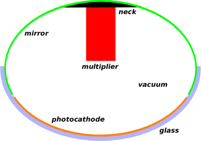
Figure 1: Schema of the advanced simulation model. The main components of the simulation set-up are the window glass, photocathode, mirror, effective absorption by the neck, and the multiplier structure.

The geometry set-up of the advanced simulation model is shown in Fig. 1. The whole shape is approximated with a full oblate spheroid with a mirrored back wall reaching $30\,\mathrm{mm}$ below the center. The reflectivity of the mirror is set to 97% and only ideal specular reflection is implemented. As in the case of the real PMTs, the photocathode on the inner side of the glass is separated from the mirror coating by a transparent gap of $5\,\mathrm{mm}$.

3.1 Inner structure of the PMT

The loss of photons in the extended neck leading to the PMT base is simulated by the 100% absorbing patch with a radius of $40\,\mathrm{mm}$ placed at the top of the PMT. The multiplier structure (dynode stack) reaches well into the center of the PMT and is in this particular PMT enclosed in a metallic shield case of cylindrical shape. In the photon-tracking experiments we have found that the proper inclusion of this multiplier volume can greatly influence the number of reflected photons (see Fig. 4 for a clear demonstration on how the parallel beam of light gets focused into the multiplier volume). The multiplier structure is thus simulated with a cylinder of height $60\,\mathrm{mm}$ and radius $16\,\mathrm{mm}$. It is made of a copper-like metal and its effective reflectivity is set to 30% (for simplicity specular reflection only).

3.2 Optical properties of the PMT glass

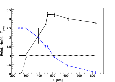
Figure 2: Real (full line) and negative imaginary (dashed line) parts of the complex refraction index of the photocathode as a function of the wavelength. The triangles are experimental data points extracted from [13]. The crosses are extrapolated values. The dotted line represents the Fermi function used to model the transmission factor of the PMT glass.

The material of the glass window limits the spectral sensitivity in the short wavelength region. The borosilicate glass has a cut-off wavelength of $270\,\mathrm{nm}$ (the point where it decreases below 10%). We have modeled this property with a simple transmission factor $T_{\text{glass}}$ that is imposed upon the entering photons,

$$T_{\text{glass}}=\exp[-d/L(\lambda)]=\operatorname{F}(\lambda;\lambda_{\text{m}},\Delta\lambda),$$ (1)

where $d$ is the thickness and $L(\lambda)$ is the absorption length of the PMT glass. The final transmission factor is modeled with a Fermi-function dependence on the wavelength, $\operatorname{F}(\lambda;\lambda_{\text{t}},\Delta\lambda)=1/(\exp[(\lambda_{\text{t}}-\lambda)/\Delta\lambda]+1)$ with $\lambda_{\text{t}}=285\,\mathrm{nm}$ for the transition wavelength and $\Delta\lambda=8\,\mathrm{nm}$ for the transition width [14] (see dotted line in Fig. 2).

3.3 Photocathode as a thin film

The sensitivity of the different types of photocathodes is restricted by the photo-emission threshold for the long wavelengths and can vary with thickness at the short wavelengths. The bi-alkali component KCsSb is practically the universal choice of photocathode material for Cherenkov light applications, and although it has been known for almost five decades, the availability of reliable measurements of index of refraction has been rather scarce. In our simulation of the angular and wavelength dependencies of the quantum efficiency we have used the data points from the experimental compilation of the complex index of refraction from [13], where the optical properties of this bi-alkali material of similar thickness have been reviewed for the purposes of the solar neutrino detector SNO. Due to the limited number of different wavelength measurements we have used a simple linear interpolation of the complex index of refraction with wavelength extension along the lines of newer experimental results from [15] (see Fig. 2).

3.4 Photoelectron production

When the photon reaches the thin layer of the photocathode it can either get reflected with probability $R$, it can get transmitted across the layer with effective probability $T$, or it can get absorbed by the photocathode material with probability $A=1-R-T$. If the photon energy in the latter case is larger than the needed exit work, the electron can leave the photocathode. The corresponding quantum efficiency $q_{\text{pc}}$ of the photocathode surface can thus be written as

$$q_{\text{pc}}(\lambda,\theta)=A(\lambda,\theta)\,p_{\text{conv}},$$ (2)

where $A(\lambda,\theta)$, the absorption coefficient, depends on incidence angle $\theta$ and wavelength $\lambda$, and $p_{\text{conv}}$ is the conversion factor. The conversion factor $p_{\text{conv}}$ does not depend on the angle of incidence [16, 17] but in principle it can still be wavelength dependent [18]. Due to the relatively narrow window of relevant wavelengths imposed by the water absorption (see Fig. 3) we approximate the conversion factor $p_{\text{conv}}$ for the purposes of our simulations with a constant. In section 3.7, we determine its effective value from the separate simulation of the quantum efficiency experiment, along the lines of the experiments usually performed by the PMT manufacturers. In the next section we will derive the second missing parameter $A(\lambda,\theta)$.

At this point it is worth to mention that the quantum efficiency $q_{\text{pc}}$ from Eq. (2) is the quantum efficiency of the photocathode surface and is only indirectly related to the overall quantum efficiency of the PMT, as found in the specifications of the manufacturers. The main difference comes from the fact that PMTs are designed to increase light collection through reflections on the mirror back wall. This increase is to some degree contained in the PMT specification. Nevertheless, its magnitude depends substantially on the particular way the quoted efficiency is obtained experimentally. Therefore, the quoted efficiency specifications of the PMT always require proper interpretation when used for a photocathode simulation. This fact is in general relevant also for other physics experiments involving PMTs.

3.5 Thin-film Fresnel equations

Studies on PMTs usually follow [19] to derive the angular and wavelength dependence of the optical properties. Here, we follow the more concise derivation from [20] that is specifically dedicated to thin film treatment. Furthermore, we adopt from [20] the sign convention for the imaginary part of the index of refraction (see Fig. 2).

Although our PMT has only one layer of thin-film photocathode, we will for the sake of clarity derive Fresnel equations for a stack of $m$ thin-film surfaces with corresponding thicknesses $d_{j}$ and indexes of reflection $n_{j}$. The indexes $n_{j}$ vary with different wavelengths but in the expressions below we do not explicitly notate the dependence on $\lambda$ for the sake of clarity. This stack of thin films is on the in-going and out-going side surrounded by two semi-infinite substrates with indexes $n_{\text{in}}$ and $n_{\text{out}}$, respectively.

The angles of refraction in the consequent layers can all be obtained from the incidence angle $\theta_{\text{in}}$ from Snell’s law

$$n_{j}\cos\theta_{j}=\sqrt{n_{j}^{2}-n_{\text{in}}^{2}\sin^{2}\theta_{\text{in}}}.$$ (3)

This expression should be used for all $m$ layers $j=1\ldots m$ even when it produces a complex cosine both in case of a complex index $n_{j}$ or a total internal reflection $n_{j}<n_{\text{in}}\sin\theta_{\text{in}}$. Phase change in the layer $j$ is denoted by

$$\delta_{j}=2\pi\frac{d_{j}}{\lambda}n_{j}\cos\theta_{j}.$$ (4)

In the case of thin layers, the transmitted and reflected light combine coherently and the vector of normalized emergent fields $\mathbf{f}_{\text{out}}$ can be expressed as in [20] with characteristic matrices of $m$ stacked layers as

$$\mathbf{f}_{\text{out}}=\begin{bmatrix}f_{E}\\ f_{H}\end{bmatrix}=\left(\prod_{j}^{m}\begin{bmatrix}\cos\delta_{j}&i\sin\delta_{j}/\eta_{j}\\ i\eta_{j}\sin\delta_{j}&\cos\delta_{j}\end{bmatrix}\right)\begin{bmatrix}1\\ \eta_{\text{out}}\end{bmatrix},$$ (5)

where $f_{E}$ and $f_{H}$ are normalized electrical and magnetic fields, respectively, and $\eta_{j}$, $\eta_{\text{out}}$ are the tilted optical admittances. Using short-hand notation for scalar products

$$t=\mathbf{f}_{\text{out}}\cdot\begin{bmatrix}\eta_{\text{in}}\\ 1\end{bmatrix}\qquad\text{and}\qquad r=\mathbf{f}_{\text{out}}\cdot\begin{bmatrix}\eta_{\text{in}}\\ -1\end{bmatrix}/t,$$ (6)

the reflectance is expressed as

$$R=r\,r^{*}=|r|^{2}=\frac{|f_{E}|^{2}\eta_{\text{in}}^{2}-2\operatorname{Re}[f_{E}f_{H}^{*}]\eta_{\text{in}}+|f_{H}|^{2}}{|t|^{2}}$$ (7)

and the transmittance as

$$T=4\eta_{\text{in}}\frac{\operatorname{Re}[\eta_{\text{out}}]}{|t|^{2}}.$$ (8)

Absorptance follows from

$$A=4\eta_{\text{in}}\frac{\operatorname{Re}[f_{E}f_{H}^{*}-\eta_{\text{out}}]}{|t|^{2}}.$$ (9)

The three quantities obey the relation $R+T+A=1$. Note that while $\eta_{\text{in}}$ is always real, $\eta_{j}$ can be complex due to absorption, and $\eta_{j}$, $\eta_{\text{out}}$ can become complex when the incidence angle $\theta_{\text{in}}$ increases above the angle of total internal reflection $\theta_{j}^{\text{tot}}$ defined by $\sin\theta_{j}^{\text{tot}}=n_{j}/n_{\text{in}}$.

The equations above have to be considered for two polarization cases. Using the convention where p-polarization implies a magnetic field component parallel to the interface boundary (TM wave) and s-polarization implies a parallel electric component (TE wave), two variants of the admittance emerge,

$$\eta_{j}^{\text{p}}=n_{j}/\cos\theta_{j}\qquad\text{and}\qquad\eta_{j}^{\text{s}}=n_{j}\cos\theta_{j},$$ (10)

where $\cos\theta_{j}$ is again obtained from Eq. (3). The same polarization cases should also be used on $\eta_{\text{in}}$ and $\eta_{\text{out}}$. The upper expressions in (7), (8), and (9) thus have to be separately evaluated for the p- and s-polarization; hence the obtained reflectance, transmittance, and absorptance change accordingly into $R_{\text{p,s}}$, $T_{\text{p,s}}$, and $A_{\text{p,s}}$. For unpolarized light we can define average quantities $R=\tfrac{1}{2}(R_{\text{p}}+R_{\text{s}})$, $T=\tfrac{1}{2}(T_{\text{p}}+T_{\text{s}})$, and $A=\tfrac{1}{2}(A_{\text{p}}+A_{\text{s}})$ which, as before, satisfy $R+T+A=1$.

Cherenkov light from the injected muon is polarized perpendicularly to the emission cone. The rotational symmetry around the muon track and the fact that after several reflections on the inner walls the photon polarization is after $\sim 30\,\mathrm{ns}$ completely randomized, enable us to use the above polarization-averaged expressions for reflectance, transmittance, and absorptance.

Figure 3: Wavelength dependency of the water absorption length $L$ and the reflectivity $R$ of the container walls. Data taken from [21] and [22], respectively.

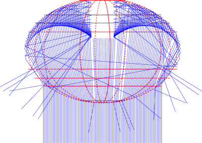
Figure 4: Simulation of the Photonis quantum efficiency experiment for estimation of the conversion factor. Absolutely calibrated parallel beam of light is sent to the front of the PMT (photocathode is at bottom of the oval). Due to the reflection on the ellipsoidal mirror at the back of the PMT, the light gets approximately focused at the position of the multiplier (caustics at the sides of the multiplier). The inclusion/exclusion of the multiplier volume can have great effect on the amount of the light returned to the photocathode surface and thus has to be properly simulated. In this figure the multiplier (c.f. white patch at top center) is obscuring most of the returning light in this configuration of the incoming beam.

3.6 Simulation set-up

The simulation of the PMT has been implemented within the Auger $\overline{\textrm{Off}}$ $\underline{\textrm{line}}$ software framework [23] where the water-Cherenkov detector simulation is implemented with the Geant4 toolkit [24]. The production of the Cherenkov light by the injected vertical-centered muons, the consequent absorption of the photons in the water, and the tracking of the photons and their reflections on the container walls have been assigned to the Geant4 part of the simulation with parametrizations shown in Fig. 3. The entry of the photons into the glass of the PMT window was also handled by Geant4. From this point on, the photons were tracked by our simulation model, based on the considerations made in the previous sections. Using the index of refraction parametrization from Fig. 2 for $n_{1}$, the individual photons were reflected from the photocathode with the probability following from the (polarization-averaged) reflectance in Eq. (7), or transmitted according to Eq. (8) into the vacuum ($n_{\text{out}}=1$) of the PMT. The simulation proceeded with the photon tracking inside the PMT which can, upon successful reflections on the inner structure, produce another crossing of the photocathode (this time with the exchanged values for the “in” and “out” variables in the upper equations) and reentry into the water. In case of an absorption of the photon upon the crossing of the photocathode, the associated photoelectron is produced according to the quantum efficiency in Eq. (2).

3.7 Calibration of the conversion factor

For the wavelength of $375\,\mathrm{nm}$, Photonis [11] quotes a value of quantum efficiency of the PMT as $q_{\text{pmt}}=0.26$. They perform the measurement with an absolutely-calibrated parallel beam of light with a diameter of $170\,\mathrm{mm}$ illuminating the front of the PMT along the PMT axis. Correcting for the 70% collection efficiency (obtained from their own electric field simulations [14]), they consequently convert the measured current into a released photoelectron flux $\Phi_{\text{pe}}$. Their definition of PMT quantum efficiency is then $q_{\text{pmt}}=\Phi_{\text{pe}}/\Phi$ where $\Phi$ is the incident photon flux from the absolutely calibrated beam.

We have reproduced this exact experimental setup and the beam geometry in our PMT simulation (see Fig. 4) in order to “reverse engineer” the PMT quantum efficiency $q_{\text{pmt}}$ into the photocathode quantum efficiency $q_{\text{pc}}$. While using the surface quantum efficiency expression from Eq. (2) we simulated a large number $N$ of the $375\,\mathrm{nm}$ photons in the incident beam and recorded the number of released photoelectrons $N_{\text{pe}}$. To reproduce the quoted PMT quantum efficiency $q_{\text{pmt}}=0.26$ with our simulated fraction $N_{\text{pe}}/N$, the conversion factor in Eq. (2) had to be set to $p_{\text{conv}}=0.405$. Thus, in effect, at $\lambda=375\,\mathrm{nm}$ slightly more than 40% of the absorbed photons in this geometry get converted to photoelectrons.

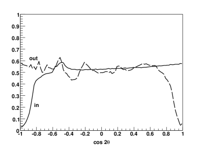
Figure 5: Normalized distribution of photons arriving to the photocathode as a function of $\cos 2\theta$ where $\theta$ is the incidence angle, for two populations, incoming (i.e. entering the PMT, full line) and outgoing (i.e. exiting the PMT, dashed line) photons. Due to the increased reflectivity of the water–glass interface a depletion from the isotropic distribution is observed for large incidence angles ($\cos(2\times 90^{\circ})=-1$) of incoming photons. For the outgoing photons the small incidence angles ($\cos(2\times 0^{\circ})=1$) are suppressed due to the reflection and absorption on the inner structure of the PMT. Note that the distribution for isotropic arrivals as a function of $\cos 2\theta$ is constant and equals to 1/2.

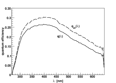
Figure 6: Quantum efficiency $q$ (full line) defined as the probability for a photon to free an electron at the photocathode crossing. The dashed line corresponds to the effective quantum efficiency $q_{\text{eff}}$, i.e. the probability for an incoming photon to eventually free an electron. The effective quantum efficiency is used in the implementation of the simplified PMT model.

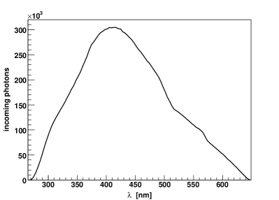
Figure 7: Photon spectrum reaching the photocathode for 10 000 injected vertical-centered muons. The main features of the curve are due to the shape of the Cherenkov emission spectrum, the wavelength dependency of the water absorption length (hump at $\sim 420\,\mathrm{nm}$), the wavelength dependence of the reflectivity of the inner walls, and the PMT glass transparency (cut-off at wavelengths $<280\,\mathrm{nm}$).

3.8 Quantum efficiency

Using the obtained conversion factor $p_{\text{conv}}=0.405$, the PMT simulation is run for a large number of injected vertical-centered muons. Fig. 5 shows the distribution of the incidence angle on the photocathode for photons entering (incoming) and exiting (outgoing) the PMT. On each crossing of the photocathode, absorbtance $A(\lambda,\theta)$ is obtained form the Eq. (9) and the photoelectron is released with probability $A(\lambda,\theta)\,p_{\text{conv}}$, as given by Eq. (2). We can derive the overall, incidence-angle averaged quantum efficiency of our PMT simulation model by dividing the number of released photoelectrons $N_{\text{pe}}$ by the number of photons $N$ reaching the photocathode (from any side) for the different wavelengths,

$$q(\lambda)=\frac{N_{\text{pe}}(\lambda)}{N(\lambda)}.$$ (11)

The resulting quantum efficiency is shown in Fig. 6 (full line). This quantum efficiency, obtained indirectly from the refractive index parametrization in Fig. 2, reproduces well the known features of other experimental data [15] and the specification of the PMT manufacturer [11]. Furthermore, it gives the correct estimates of the average number of photoelectrons released by the traversing muon as measured in scintillator-triggered experiments with Auger SD stations [2, 3].

4 Relevance to other astrophysics experiments

There are several important points that can be extracted from the previous sections. For optical interfaces, the Geant4 framework implements only the familiar Fresnel equations of geometrical optics and does not include the physical optics relevant for a thin-film photocathode, as given by Eqs. (5–9). The dependence of the photocathode absorption (and consequently of the quantum efficiency) on the incidence angle is correctly described only by the thin-film equations which have to be implemented independently of Geant4. The absorption increases up to 50% for incidence angles larger than the angle of total internal reflection for the glass–vacuum interface. No such increase is observed for the reverse, vacuum–glass transition of the photons. Furthermore, the quantum efficiency obtained from the manufacturer’s calibration setup already contains a nontrivial fraction of the efficiency increase due to the reflectivity of the inner structure of the PMT. The “intrinsic” quantum efficiency of the photocathode layer thus has to be reverse-engineered by a procedure similar to the one described in Section 3.7. Clearly, both effects are most relevant in cases of experiments with a distribution of incoming photons substantially different from those characteristic of manufacturer’s experimental setup.

This may be of relevance to experiments employing similarly large PMTs in various Cherenkov detectors, like Amanda, IceCube, and IceTop [25, 26, 27], Kamiokande [28], NESTOR, NEMO, and Antares [29, 30, 31], MiniBooNE [32], Xenon [33], Baikal and Tunka [34], and northern Auger Observatory [35], just to name a few.

5 Simplified simulation model

In a simulation, a vertical-centered muon injected into the water of the SD station has a $1.2\,\mathrm{m}$ tracklength and typically releases $\sim 67\,500$ Cherenkov photons in the energy range between 1.5 and $5\,\mathrm{eV}$ (250 to $830\,\mathrm{nm}$ in wavelength; see Fig. 7 for spectrum). Additional $\sim 10\%$ of photons get produced by the secondary delta rays, in total giving $\sim 73\,100$ photons per muon. All these photons require a complete tracking inside the water container by Geant4. The photons on their way undergo the absorption in the water medium, get reflected and absorbed by the container walls. On average, only $\sim 1340$ (1.8%) of all photons eventually reach the PMT photocathode. As described in the previous sections, the photon tracks are then simulated inside the PMT and the probability of a photoelectron release is evaluated. A large fraction of produced photons will never reach the PMT and additionally a fraction of the incoming photons will be absorbed without producing any photoelectrons. To avoid the time-consuming simulation of these photons that do not contribute to the PMT signal, a simplified simulation has been devised. The goal is to estimate the effective probability for an emerging photon to contribute to the signal and eliminate idle photons from the simulation. The corresponding statistical thinning can thus be applied already at the time of their production.

5.1 Effective quantum efficiency for incoming photons

After several reflections on the walls, the swarm of photons behaves similarly to a photon gas. As can be already seen from the incidence-angle distribution of photons on the photocathode (see Fig. 5), the distribution of arrival directions is close to isotropic. Instead of the detailed simulation of photon tracks inside the advanced PMT model we can reduce the complexity of the procedure by introducing the simplified model of the PMT. The quantum efficiency in Eq. (11) stemming from Fresnel equations of the advanced PMT model is replaced with an effective quantum efficiency $q_{\text{eff}}$ that describes the probability for an incoming photon to produce a photoelectron,

$$q_{\text{eff}}(\lambda)=\frac{N_{\text{pe}}(\lambda)}{N_{\text{in}}(\lambda)}.$$ (12)

The $q_{\text{eff}}$ is obtained from the advanced model by normalizing the statistics of the released photoelectrons by the number of incoming photons. The actual wavelength dependence of $q_{\text{eff}}(\lambda)$ is shown in Fig. 6 (dashed line).

In the advanced model only 4.5% of the incoming photons return to the water medium, i.e. only 0.08% of all produced photons. In Fig. 8, a wavelength-resolved fraction of outgoing vs. incoming photons is shown. The fraction is as low as 2% for short wavelengths and does not exceed 22% for long wavelengths.

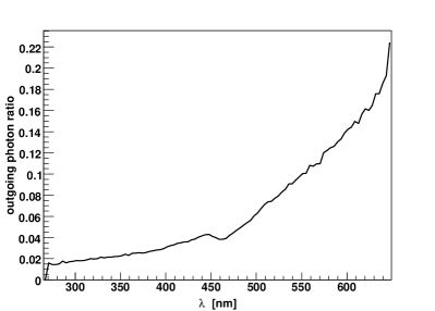
Figure 8: Ratio of outgoing vs. incoming photons as counted at the PMT photocathode.

Figure 9: Representation of the simplified model of PMT.

Based on these facts we have developed an implementation of the simplified PMT model that uses only a rudimentary geometry as shown in Fig. 9. In this simplified model the photons are detected on contact with the outer surface and are consequentially removed from the simulation. No tracking of the photons on the inner structure of the PMT is performed. The chance of producing a photoelectron on the second crossing of the photocathode in the advanced model is accounted for in the simplified model by the usage of the effective quantum efficiency from Eq. (12). The relative ratio of the quantum efficiencies from Eqs. (12) and (11) is shown in Fig. 10. The ratio is mostly close to $\sim 10\%$ increase but then gradually climbs to $\sim 35\%$ for long wavelengths.

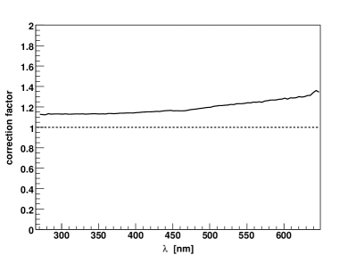
Figure 10: Correction factor $q_{\text{eff}}(\lambda)/q(\lambda)$ as a function of the wavelength. For short wavelengths the correction is of the order of 13% and goes up to 35% for long wavelengths.

5.2 Statistical thinning

Similar to the well established method in extensive air-shower simulations [36, 37], the concept of effective quantum efficiency enables us to implement efficient statistical thinning of the simulated photons. At the moment of production, out of $N_{\text{pr}}(\lambda)$ photons with wavelength $\lambda$ only $q_{\text{eff}}(\lambda)N_{\text{pr}}(\lambda)$ photons with weight $1/q_{\text{eff}}(\lambda)$ undergo further simulation. As a result, such thinned photons upon reaching the photocathode have to produce a photoelectron with probability 1. The average quantum efficiency (in photon energy scale where Cherenkov spectrum is flat) is $\bar{q}_{\text{eff}}=0.22$, resulting in a simulation speed-up for almost a factor $\sim 5$. If we take into account also the losses due to the PMT collection efficiency, this number increases to $\sim 6.5$.

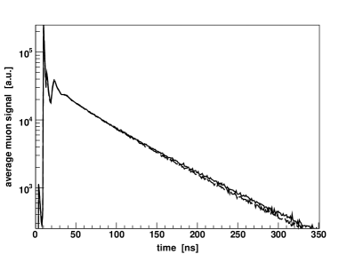
Figure 11: Comparison of the time dependence of the muon signal in an SD station for the advanced PMT model (full line) and the simplified version (dashed line). The main feature is an approximate exponential time dependence with a decay time $\tau\approx 65\,\mathrm{ns}$. The two models agree well with respect to the small details of the early signal and the latter decay part. A small discrepancy, limited to less than 5%, is observed only in the late tail. Note that the oscillating structure for time $<30\,\mathrm{ns}$ is due to the nonuniform arrival of photons after the first few reflections when photons can not be treated yet as homogeneous and isotropic photon gas.

In Fig. 11 the results for the muon response in SD station is compared for both models. The main feature is an exponential decay but with a slightly changing exponent due to the wavelength dependence of the water absorption and wall reflectivity. The characteristic decay time of the muon signal is around $\tau\approx 65\,\mathrm{ns}$. Except in the tail of relatively large times, $t\gg\tau$, where the discrepancy is limited to within 5%, the simplified model reproduces well the details of the muon signal from the advanced PMT model, especially the overall exponential decay and an oscillatory behavior for $t<20\,\mathrm{ns}$. It is worth mentioning here that the signal from the PMT in an SD station is sampled with a $40\,\mathrm{MHz}$ ($25\,\mathrm{ns}$) FADC, i.e. all these details will lie within one sampling bin.

6 Summary

We have implemented an advanced model for the simulation of the PMT response in a water-Cherenkov station of the surface detector. The model is based on the correct thin-film treatment of the photocathode optical processes with complex index of refraction. The model also includes tracking of the photons on the inner mirror surfaces and multiplier structure.

To relate the obtained quantum efficiency of the photocathode to quoted efficiency from the PMT specification we have in simulation reproduced the experimental set-up of the measurement done by the manufacturer. This properly accounts for the increase in photon collecting due to the reflections on mirrored surfaces and inner structure of the PMT, and gives the average value of the conversion factor.

Since a relatively large number of photons is involved in the creation of the muon signal, certain details of the simulation, like the dependence of the absorption on the incidence angles and the exact tracking of the photons on the inner structure, are washed out and can be treated in a phenomenological way.

To reduce the simulation time as well as the complexity of the problem we have implemented another, simplified model of the PMT. Results for the average photoelectron release probabilities for different wavelengths in the advanced PMT model were in turn used to calibrate the effective quantum efficiency of the simplified model. Results from both models agree well with the experimentally obtained number of produced photoelectrons per muon injection. Finally, we have shown that the time dependence of the muon signal is almost not affected by the simplification in the simulation strategy.

References

- [1] J. Abraham, et al., Nucl. Instr. and Meth. A 523 (2004) 50.
- [2] M. Aglietta, et al., in: Proceedings of the 29th International Cosmic Ray Conference 7 (2005) 83; P.S. Allison, et al., in: ibid. 8 (2005) 299; P.L. Ghia, et al., in: Proceedings of the 30th International Cosmic Ray Conference 4 (2007) 315.
- [3] P.S. Allison, et al., in: Proceedings of the 29th International Cosmic Ray Conference 7 (2005) 357; T. Dova, et al., in: ibid. 7 (2005) 5.
- [4] P.K.F. Grieder, Cosmic Rays at Earth, Elsevier, Amsterdam, 2001, p. 354.
- [5] R. Engel, et al., in: Proceedings of the 30th International Cosmic Ray Conference 4 (2007) 385.
- [6] M. Healy, et al., in: Proceedings of the 30th International Cosmic Ray Conference 4 (2007) 377; ibid. 381.
- [7] J. Abraham, et al., Astropart. Phys. 29 (2008) 243; arXiv:0712.1147 [astro-ph].
- [8] A.K. Tripathi, et al., in: Proceedings of the 28th International Cosmic Ray Conference (2003) 1041.
- [9] P.L. Ghia, et al., in: Proceedings of the 30th International Cosmic Ray Conference (2007); arXiv:0706.1212 [astro-ph].
- [10] P. Billoir, Astropart. Phys. 30 (2008) 270.
- [11] Photonis Photomultiplier Tubes Catalogue, http://www.photonis.com/industryscience/products/photomultipliers_assemblies/pmt_catalogue.
- [12] B. Genolini, et al., Nucl. Instr. and Meth. A 504 (2003) 240.
- [13] M.E. Moorhead, N.W. Tanner, Nucl. Instr. and Meth. A 378 (1996) 162.
- [14] S.-O. Flyckt, C. Marmonier, Photomultiplier tubes – principles & applications, Photonis, 2002, http://www.photonis.com/industryscience/products/photomultipliers_assemblies/application_book_1.
- [15] D. Motta, S. Schonert, Nucl. Instr. and Meth. A 539 (2005) 217.
- [16] M.D. Lay, Nucl. Instr. and Meth. A 383 (1996) 485.
- [17] T.H. Chyba, L. Mandel, J. Opt. Soc. Am. B 5 (1988) 1305.
- [18] M.D. Lay, M.J. Lyon, Nucl. Instr. and Meth. A 383 (1996) 495.
- [19] M. Born, E. Wolf, Principles of Optics, 7th Edition, Cambridge University Press, 1999.
- [20] H.A. Macleod, Thin-Film Optical Filters, third edition, Institute of Physics Publishing, Bristol, 2001.
- [21] R.C. Smith and K.S. Baker, Appl. Opt. 20 (1981) 177.
- [22] Surface Optics Corporation, Report SOC-R950-001-0195.
- [23] S. Argirò, et al., Nucl. Instr. and Meth. A 580 (2007) 1485.
- [24] S. Agostinelli, et al., Nucl. Instr. and Meth. A 506 (2003) 250.
- [25] J. Ahrens, et al., Nucl. Instrum. Meth. A 524 (2004) 169.
- [26] A. Achterberg, et al., Astropart. Phys. 26 (2006) 155.
- [27] T. Stanev, R. Ulrich, et al., in: Proceedings of the 28th International Cosmic Ray Conference (2003) 965.
- [28] Y. Totsuka, Nucl. Phys. Proc. Suppl. B 48 (1996) 547.
- [29] E.G. Anassontzis, et al., Nucl. Instrum. Meth. A 479 (2002) 439.
- [30] E. Migneco, et al., Nucl. Phys. Proc. Suppl. B 136 (2004) 61.
- [31] P. Amram, et al., Nucl. Instrum. Meth. A 484 (2002) 369.
- [32] S.J. Brice, et al., Nucl. Instrum. Meth. A 562 (2006) 97.
- [33] E. Aprile, et al., in: International Workshop on Techniques and Applications of Xenon Detectors (2001); arXiv:astro-ph/0207670.
- [34] R.I. Bagduev, et al., Nucl. Instrum. Meth. A 420 (1999) 138; B.K. Lubsandorzhev, et al., Nucl. Instrum. Meth. A 442 (2000) 368.
- [35] D.Nitz, et al., in: Proceedings of the 30th International Cosmic Ray Conference 5 (2007) 889.
- [36] A.M. Hillas, Nucl. Phys. Proc. Suppl. B 52 (1997) 29.
- [37] J. Knapp, D. Heck, S.J. Sciutto, M.T. Dova, and M. Risse, Astroparticle Phys. 19 (2003) 77.