Cooling a mechanical resonator by quantum interference in a triple quantum dot

Abstract

We propose an approach to cool a mechanical resonator (MR) via quantum interference in a triple quantum dot (TQD) capacitively coupled to the MR. The TQD connected to three electrodes is an electronic analog of a three-level atom in $\Lambda$ configuration. The electrons can tunnel from the left electrode into one of the two dots with lower-energy states, but can only tunnel out from the higher-energy state at the third dot to the right electrode. When the two lower-energy states are tuned to be degenerate, an electron in the TQD can be trapped in a superposition of the degenerate states called the dark state. This effect is caused by the destructive quantum interference between tunneling from the two lower-energy states to the higher-energy state. Under this condition, an electron in the dark state readily absorbs an energy quantum from the MR. Repeating this process, the MR can be cooled to its ground state. Moreover, we propose a scheme for verifying the cooling result by measuring the current spectrum of a charge detector adjacent to a double quantum dot coupled to the MR.

I Introduction

Mechanical resonators (MRs) with a high resonant frequency and a small mass have wide applications and are attracting considerable recent attentions Huang03 ; Schwab05 . Technically, these MRs can be used as ultrasensitive sensors in high-precision displacement measurements LaHaye04 , detection of gravitational waves BraginskyPLA02 or mass detection Buks06 . Also, quantized MRs can be useful in quantum information processing. Indeed, quantized motion of buckling nanoscale bars has been proposed for qubit implementation SavelNJP ; Savel07 and also for creating quantum entanglement Vitali07 ; Hartmann08 ; Tian04 . However, for all these applications, a basic prerequirement is that the dynamics of the MRs must approach the quantum regime.

Quantum behaviors of a MR are usually suppressed by the coupling to its environment. One way to approach the quantum regime is to increase its resonant frequency so that an energy quantum of the MR becomes larger than the thermal energy. Recently, MRs based on metallic beams TF08 and carbon nanotubes Huttel09 have been developed, which have resonance frequencies of several hundred megahertz. However, for a MR with a frequency of $200$ MHz, a temperature lower than $10$ mK (below the present dilution refrigerator temperature) is required to maintain the MR at the quantum regime. To attain the quantum regime, one needs to cool the MR further via coupling to an optical or an on-chip electronic system. Numerous experiments on cooling a single MR via radiation pressure or dynamical backaction have been reported (see, e.g., Metzger04 ; Gigan06 ; Kleckner06 ; Arcizet06 ; Naik06 ; Schliesser06 ; Poggio07 ; Lehnert08 ; Kippenberg05 ). Theoretically, cooling by coupling to a Cooper pair box Zhang05 or to a three-level flux qubit You08 via periodic resonant coupling have also been proposed. In these schemes, a strong resonant coupling between the MR and the qubit is required to cool the MR to its ground state.

I.1 Sideband cooling of a MR

In the weak coupling regime, a conventional method for cooling the MR is the sideband cooling approach (see, e.g., Ref. Wilson04 ; Wilson07 ; Marquardt07 ; ASchliesser08 ; Yong08 ; Ouyang09 ; Zippilli09 ; Grajcar08 ). In this case, a MR is coupled to a two-level system (TLS) in which the two states can be electronic states in quantum dots Wilson04 ; Ouyang09 ; Zippilli09 , photonic states in a cavity Wilson07 ; Marquardt07 ; ASchliesser08 ; Yong08 , or charge states in superconducting qubits You05 . In order to achieve ground-state cooling in the sideband cooling approach, the resolved-sideband cooling condition $\omega_{m}\gg\Gamma$ (with $\omega_{m}$ denoting the oscillating frequency of the MR and $\Gamma$ the decay rate of the TLS) must be followed in order to selectively drive the lowest sideband of the TLS. Then, the excitation of the TLS from the ground state $|g\rangle$ to the excited state $|e\rangle$ and the subsequent decay from this excited state to the ground state will, on average, decrease an energy quantum in the MR. This process can be described by $|g,n\rangle\rightarrow|e,n-1\rangle\rightarrow|g,n-1\rangle$, where $n$ denotes to the state with $n$ phonons. However, the frequency of a typical MR is about $100$ MHz TF08 ; Huttel09 . It is in general of the same order of the decay rate of the two-level system. This indicates that the resolved-sideband cooling condition is not easy to fulfill. Violating the condition means that the processes of a carrier transition and a subsequent sideband transition (i.e., $|g,n\rangle\rightarrow|e,n\rangle\rightarrow|g,n+1\rangle$) will occur. This will heat up the MR instead and suppress any ground-state cooling ASchliesser08 .

I.2 Cooling atomic motion via quantum interference in a three-level atom

For laser cooling of atoms, an alternative approach Morigi00 based on quantum interference in the internal degrees of freedom of the atoms without the need to follow the resolved-sideband cooling condition has been proposed. In this approach, an additional state is coupled to the excited state $|3\rangle$ of the TLS to form a $\Lambda$-shaped three-level system [see Fig. 1(b)]. The two lower-energy states in this three-level system are tuned to be degenerate. Due to dissipation of the excited state, the atom will eventually arrive at a particular superposition of the two lower-energy states which is orthogonal to the excited state. This phenomenon results from the destructive quantum interference between the two transitions $|1\rangle\rightarrow|3\rangle$ and $|2\rangle\rightarrow|3\rangle$ and the superposition state is called the dark state Scully . When atomic motion is also considered, the carrier transition ($|1,n\rangle\rightarrow|3,n\rangle$) and thus the heating process of the atomic motion in the sideband cooling scheme is hence suppressed. It was shown that atomic motion can be cooled to its ground state in the non-resolved sideband regime Morigi00 .

I.3 Cooling a MR via quantum interference in a triple quantum dot

In the present work, we propose a new scheme to cool a MR via capacitive coupling to a triple quantum dot (TQD) schematically displayed in Fig. 1(a). We consider the strong Coulomb-blockade regime so that at most one electron is allowed to present at one time in the TQD. The TQD acts as a three-level system in $\Lambda$ configuration, in which the two dot states $|1\rangle$ and $|2\rangle$ (i.e., the single-electron orbital states in dots 1 and 2) are coupled to a third (excited) state $|3\rangle$ via two tunnel barriers [see Fig. 1(a)]. Here, the degrees of freedom of the MR is analogous to the motional degrees of freedom of the atoms discussed above and the TQD is an electronic analog of a three-level atom. We will show that by properly tuning the gate voltages, one can degenerate the two lower-energy states and obtain a dark state in the TQD. By capacitively coupling to the TQD, the MR can be cooled to its ground state, in full analogy to the slowing down of the atoms via quantum interference. Comparing with the cooling of atoms Morigi00 , our approach has the following potential advantages: (i) Our cooling system is completely electronic and can be conveniently fabricated on a chip. (ii) Simply by adjusting the gate voltages, it is easy to achieve the two degenerate lower-energy states required for realizing destructive quantum interference in the TQD. Moreover, in contrast to the cooling of a MR by coupling it to a superconducting qubit Xia09 , the decay rate $\Gamma$ of the higher-energy state of the TQD, which is equal to the rate of electrons tunneling from the TQD to the electrode, is tunable in our case by varying the gate voltage.

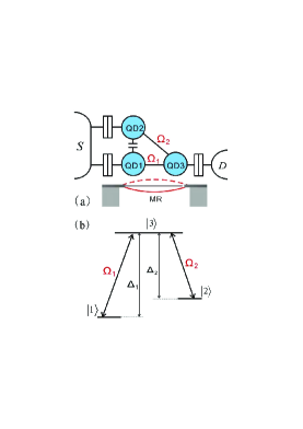
Figure 1: (color online) Schematic diagram of a TQD system. Dots $1$ and $2$ are both tunnel-coupled to dot $3$ (with interdot coupling strengths $\Omega_{1}$ and $\Omega_{2}$, respectively) while they are only capacitively coupled to each other. A MR is capacitively coupled to dots $1$ and $3$ of the TQD. (b) A three-level system in $\Lambda$ configuration. The energy detunings between the two lower-energy states and the third excited state are respectively $\Delta_{1}$ and $\Delta_{2}$. The coupling strength between the state $|1\rangle$ ($|2\rangle$) and the state $|3\rangle$ is $\Omega_{1}$ ($\Omega_{2}$).

Moreover, we also propose a method to verify whether the MR is successfully cooled by coupling it to a double quantum dot (DQD). This DQD can be reduced from the TQD by applying appropriate gate voltages. When the DQD and the MR is tuned into a strongly dispersive regime in which the transition frequency difference between the two subsystems is much larger than the coupling strength between them, the coupling between the MR and the DQD only yields a phonon-number-dependent Stark shift to the transition frequency of the DQD. This Stark shift corresponds to the shift of the resonant peak in the current spectrum of a charge detector. Thus, by measuring the shift of the resonant peak, one can readout the phonon-number state and examine whether the MR is successfully cooled or not.

This paper is organized as follows. Section II introduces a microscopic model for the coupled MR-TQD system. We show that the TQD is an electronic analog of a three-level atom driven by two electromagnetic fields. Also, we show how the TQD evolves into the dark state. In Sec. III, we derive a master equation to describe the quantum dynamics of the coupled MR-TQD system. With this master equation, we further derive in Sec. IV the master equation of the MR by eliminating the TQD degrees of freedom. Moreover, we calculate the steady-state average phonon occupancy of the MR and show that the MR can indeed be cooled to its ground state by using the quantum interference in the TQD. In Sec. V, we propose a method to verify if the MR is successfully cooled by measuring the full-frequency current spectrum of a charge detector. Section VI summarizes our results. In the appendix, we give a detailed derivation of the master equation for the reduced density matrix of the MR.

II A mechanical resonator coupled to a triple quantum dot

II.1 Model

The device layout of a MR coupled to a TQD is shown in Fig. 1(a). The TQD is connected to three electrodes via tunneling barriers. In the TQD, dots $1$ and $2$ are only capacitively coupled to each other and electrons cannot tunnel directly between them. Such capacitively coupled dots have already been achieved in experiments (see, e.g., Clure07 ). In contrast, electrons can tunnel between dots $1$ and $3$ as well as between dots $2$ and $3$. Here we focus on the strong Coulomb-blockade regime, so that at most a single electron is allowed in the TQD. Thus, only four electronic states need to be considered in the TQD, i.e., the vacuum state $|0\rangle$, and states $|1\rangle$, $|2\rangle$ and $|3\rangle$ corresponding to a single electron in the respective dot. The MR is capacitively coupled to dots $1$ and $3$ and this is schematically shown in Fig. 1(a).

The total Hamiltonian of the whole system reads

$$H_{\rm{total}}\!=\!H_{0}+H_{\rm{int}}+H_{\rm{T}}+H_{\rm ep}.$$ (1)

The unperturbed Hamiltonian $H_{0}$ is defined by

$$H_{0}\!=\!H_{\rm{leads}}+H_{\rm{TQD}}+H_{\rm{R}}+H_{\rm ph},$$ (2)

where terms on the R.H.S. of Eq. (2) denote Hamiltonians of the electrodes, the TQD, the MR and the thermal bath given by

$$H_{\rm{leads}}\! =\! \sum_{ik}E_{ik}c_{ik}^{\dagger}c_{ik},$$ (3)

$$H_{\rm{TQD}}\!\! \!=\! \!\!-\Delta_{1}a_{1}^{\dagger}a_{1}\!-\!\Delta_{2}a_{2}^{\dagger}a_{2}\!+\!(\Omega_{1}a_{1}^{\dagger}a_{3}+\Omega_{2}a_{2}^{\dagger}a_{3}+{\rm H.c.}),$$

$$H_{\rm{R}}\! =\! \omega_{m}b^{\dagger}b,$$ (5)

$$H_{\rm ph}\! =\! \sum_{q}\omega_{q}b_{q}^{\dagger}b_{q}.$$ (6)

We have put $\hbar=1$ and the energy of the state $|3\rangle$ is chosen as the zero-energy point. $c_{ik}^{\dagger}$ ($c_{ik}$) is the creation (annihilation) operator of an electron with momentum $k$ in the $i$th electrode ($i=1,2$ or $3$) and $a_{i}^{\dagger}$ creates an electron in the $i$th dot. The phonon operators $b^{\dagger}$ and $b$ respectively create and annihilate an excitation of frequency $\omega_{m}$ in the MR. In Eq. (6), the thermal bath is modeled as a bosonic bath with $b_{q}^{\dagger}$ ($b_{q}$) being the creation (annihilation) operator at freqency $\omega_{q}$.

The electromechanical coupling between the MR and dots 1 and 3 of the TQD is given by

$$H_{\rm{int}}=-g\;(a_{3}^{\dagger}a_{3}-a_{1}^{\dagger}a_{1})(b^{\dagger}+b),$$ (7)

with a coupling strength $g=\eta\omega_{m}$. For a typical electromechanical coupling, $\eta$ $\sim 0.1$ (see, e.g., Ref. Neill09 ). The tunneling coupling between the TQD and the electrodes is

$$H_{\rm{T}}=\sum_{ik}(\Omega_{ik}\;a_{i}^{\dagger}\,c_{ik}+\rm{H.c.}),$$ (8)

where $\Omega_{ik}$ characterizes the coupling strength between the $i$th dot and the associated electrode via tunneling barrier. Moreover, the coupling of the MR to the outside thermal bath is characterized by

$$H_{\rm ep}=\sum_{q}\Omega_{q}(b_{q}^{\dagger}b+{\rm H.c.}),$$ (9)

with a coupling strength $\Omega_{q}$.

II.2 Analogy between TQD and $\Lambda$-type three-level atom in two driving electromagnetical fields

We now show that in the absence of the MR, our TQD system is analogous to a typical $\Lambda$-type three-level atom in the presence of two classical electromagnetical fields. This field-driven three-level system is often used in quantum optics for producing a dark state (see, e.g., Scully ). The Hamiltonian of the field-driven $\Lambda$-type three-level system can be written as

$$H_{\Lambda}\! \!=\! \!\omega_{1}a_{1}^{\dagger}a_{1}+\omega_{2}a_{2}^{\dagger}a_{2}+\omega_{3}a_{3}^{\dagger}a_{3}$$ (10)

$$+\Omega_{a}\cos(\omega_{a}t)(a_{1}^{\dagger}a_{3}+a_{3}^{\dagger}a_{1})$$

$$+\Omega_{b}\cos(\omega_{b}t)(a_{2}^{\dagger}a_{3}+a_{3}^{\dagger}a_{2}),$$

where $\omega_{i}$ ($i=1,2$ or $3$) is the energy of the $i$th state in the three-level system. Also, $\omega_{a}$ and $\omega_{b}$ are the frequencies of the two driving fields and $\Omega_{a}$ and $\Omega_{b}$ are the corresponding driving strengths. In order to eliminate the time-dependence of the Hamiltonian in Eq. (10), we transform the system into a rotating frame defined by $U_{R}=e^{iRt}$ with

$$R=\omega_{a}a_{1}^{\dagger}a_{1}+\omega_{b}a_{2}^{\dagger}a_{2}-\omega_{3}(a_{1}^{\dagger}a_{1}+a_{2}^{\dagger}a_{2}+a_{3}^{\dagger}a_{3}).$$ (11)

The transformed Hamiltonian is

$$\widetilde{H}_{\Lambda}=U_{R}^{-1}H_{\Lambda}U_{R}+i\dot{U}_{R}^{-1}U_{R},$$ (12)

where the first term is evaluated as (within the rotating-wave approximation)

$$U_{R}^{-1}H_{\Lambda}U_{R}\! \!=\! \!\omega_{1}a_{1}^{\dagger}a_{1}+\omega_{2}a_{2}^{\dagger}a_{2}+\omega_{3}a_{3}^{\dagger}a_{3}$$

$$+\frac{\Omega_{a}}{2}(a_{1}^{\dagger}a_{3}+a_{3}^{\dagger}a_{1})+\frac{\Omega_{b}}{2}(a_{2}^{\dagger}a_{3}+a_{3}^{\dagger}a_{2}),$$

and the second term gives

$$i\dot{U}_{R}^{-1}U_{R}\! = \!\omega_{a}a_{1}^{\dagger}a_{1}+\omega_{b}a_{2}^{\dagger}a_{2}-\omega_{3}(a_{1}^{\dagger}a_{1}+a_{2}^{\dagger}a_{2}+a_{3}^{\dagger}a_{3}).$$

Thus, Eq. (12) reduces to

$$\widetilde{H}_{\Lambda}\! = \!-\Delta_{1}a_{1}^{\dagger}a_{1}-\Delta_{2}a_{2}^{\dagger}a_{2}$$ (15)

$$+\Omega_{1}(a_{1}^{\dagger}a_{3}+a_{3}^{\dagger}a_{1})+\Omega_{2}(a_{2}^{\dagger}a_{3}+a_{3}^{\dagger}a_{2}),$$

where $\Delta_{1}=\omega_{3}-\omega_{1}-\omega_{a}$ and $\Delta_{2}=\omega_{3}-\omega_{2}-\omega_{b}$ are the frequency detunings while $\Omega_{1}=\Omega_{a}/2$ and $\Omega_{2}=\Omega_{b}/2$ are the effective driving strengths of the two fields. It is now clear that the Hamiltonian in Eq. (15) is formally equivalent to that of the TQD in Eq. (II.1). This shows that the TQD we propose here is an electronic analog of a $\Lambda$-type three-level atom driven by two electromagnetic fields.

II.3 “Dark state” in the TQD

From the study of quantum optics, the existence of a dark state in a $\Lambda$-type three-level atom when the lower-energy states become degenerate, i.e., $\Delta_{1}=\Delta_{2}$, is able to suppress absorption or emission. Below we demonstrate that a similar dark state also exists in the TQD Michaelis06 .

After tracing over the degrees of freedom of the electrodes, the quantum dynamics of the TQD in the absence of the MR is described by

$$\dot{\rho}_{d}\! \!=\! \!\mathcal{L}_{\rm TQD}\rho_{d}$$

$$\!=\! \!-i[H_{\rm TQD},\rho_{d}]+\Gamma_{1}\mathcal{D}[a_{1}^{\dagger}]\rho+\Gamma_{2}\mathcal{D}[a_{2}^{\dagger}]\rho_{d}+\Gamma_{3}\mathcal{D}[a_{3}]\rho_{d},$$

where $\rho_{d}$ is the reduced density matrix of the TQD and $\Gamma_{i}$ ($i=1,~{}2$ or $3$) is the rate for electrons tunneling into or out of the $i$th dot. The notation $\mathcal{D}$ for any operator $A$ is given by

$$\mathcal{D}[A]\rho=A\rho A^{\dagger}-\frac{1}{2}[A^{\dagger}A\rho+\rho A^{\dagger}A].$$ (17)

Considering equal energy detunings of the lower energy states $|1\rangle$ and $|2\rangle$ with respect to the excited state $|3\rangle$, i.e., $\Delta_{1}=\Delta_{2}=\Delta$, the eigenstates $|g\rangle$, $|-\rangle$ and $|+\rangle$ of the TQD become

$$|g\rangle \!= \!\beta|3\rangle-\frac{\alpha}{\Omega}(\Omega_{1}|1\rangle+\Omega_{2}|2\rangle),$$

$$|-\rangle \!= \!\frac{1}{\Omega}(\Omega_{2}|1\rangle-\Omega_{1}|2\rangle),$$

$$|+\rangle \!= \!\alpha|3\rangle+\frac{\beta}{\Omega}(\Omega_{1}|1\rangle+\Omega_{2}|2\rangle),$$ (18)

where $\alpha=\cos(\theta/2)$, $\beta=\sin(\theta/2)$, $\tan\theta=2\Omega/\Delta$, and $\Omega=\sqrt{\Omega_{1}^{2}+\Omega_{2}^{2}}$. The corresponding eigenenergies are

$$E_{\rm g}=-\frac{\Delta+\phi}{2},~{}~{}E_{-}=-\Delta,~{}~{}E_{+}=-\frac{\Delta-\phi}{2},$$ (19)

with $\phi=\sqrt{\Delta^{2}+4\Omega^{2}}$. For simplicity, we consider equal couplings of the three quantum dots to the corresponding electrodes, i.e., $\Gamma_{1}=\Gamma_{2}=\Gamma_{3}\equiv\Gamma$. Based on the eigenstate basis of the TQD in Eq. (II.3), the equations of motion for the reduced density matrix elements of the TQD are obtained from Eq. (LABEL:ME-TQD) as

$$\dot{\rho}_{00}\! \!=\! \!-2\Gamma\rho_{00}+\Gamma\beta^{2}\rho_{gg}+\Gamma\alpha^{2}\rho_{++}+\Gamma\alpha\beta(\rho_{+g}+\rho_{g+}),$$

$$\dot{\rho}_{gg}\! \!=\! \!\Gamma\alpha^{2}\rho_{00}-\Gamma\beta^{2}\rho_{gg}-\frac{\Gamma}{2}\alpha\beta(\rho_{+g}+\rho_{g+}),$$

$$\dot{\rho}_{--}\! \!=\! \!\Gamma\rho_{00},$$

$$\dot{\rho}_{++}\! \!=\! \!\Gamma\beta^{2}\rho_{00}-\Gamma\alpha^{2}\rho_{++}-\frac{\Gamma}{2}\alpha\beta(\rho_{+g}+\rho_{g+}),$$

$$\dot{\rho}_{+g}\! \!=\! \!-i(E_{\rm+}-E_{\rm g})\rho_{+g}-\frac{\Gamma}{2}\rho_{+g}$$ (20)

$$-\frac{\Gamma}{2}\alpha\beta(\rho_{++}+\rho_{gg})-\Gamma\alpha\beta\rho_{00}.$$

Figure 2 schematically show effective electron tunneling processes through the TQD as described by Eq. (20). Starting from an initially empty TQD, an electron can tunnel from the left electrode into any of the three eigenstates, with tunneling rates $\Gamma\beta^{2}$, $\Gamma$ and $\Gamma\alpha^{2}$ for eigenstates $|+\rangle$, $|-\rangle$ and $|g\rangle$, respectively. An electron in the eigenstate $|+\rangle$ ($|g\rangle$) then tunnels out of the TQD to the right electrode with a rate $\Gamma\alpha^{2}$ ($\Gamma\beta^{2}$). However, if the electron occupies the state $|-\rangle$, no further tunneling occurs because, being orthogonal to $|3\rangle$, it is decoupled from the right electrode. Therefore, an electron in the TQD will be trapped in the state $|-\rangle$, which is called the dark state in quantum optics Michaelis06 . This dark state results from the destructive quantum interference between the transition $|1\rangle\rightarrow|3\rangle$ (i.e., the electron tunneling from state $|1\rangle$ to state $|3\rangle$ in the TQD system) and the transition $|2\rangle\rightarrow|3\rangle$ (i.e., the electron tunneling from state $|2\rangle$ to state $|3\rangle$).

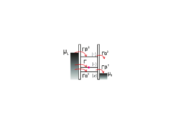
Figure 2:  (color online) Effective tunneling processes of electrons through a TQD represented in the eigenstate basis. An electron can tunnel from the left electrode into the three eigenstates $|+\rangle$, $|-\rangle$ and $|g\rangle$, with rates $\Gamma\beta^{2}$, $\Gamma$ and $\Gamma\alpha^{2}$, respectively. Note that the total tunneling rate is $2\Gamma$ because an electron tunnels from the left electrode to the TQD via two tunnel barriers (each having a tunneling rate $\Gamma$). In the eigenstate $|+\rangle$ ($|g\rangle$), it will tunnel out to the right electrode with a rate $\Gamma\alpha^{2}$ ($\Gamma\beta^{2}$). However, if the electron occupies the dark state $|-\rangle$, no further tunneling occurs and the electron is trapped.

III Effective Hamiltonian and master equation for the coupled MR-TQD system

We now study the coupled MR-TQD system. Rather than analyzing directly the energy exchange between the MR and the TQD which involves tedious algebra, we apply a canonical transform $U=e^{S}$ on the whole system, where

$$S=\eta(a_{3}^{\dagger}a_{3}-a_{1}^{\dagger}a_{1})(b-b^{\dagger}).$$ (21)

The transformed Hamiltonian is given by

$$H\! \!=\! \!UH_{\rm{total}}U^{\dagger}$$ (22)

$$\!=\! \!H_{\rm leads}+H_{\rm ph}+H_{\rm ep}+\omega_{m}b^{\dagger}b-\Delta_{1}a_{1}^{\dagger}a_{1}-\Delta_{2}a_{2}^{\dagger}a_{2}$$

$$+[\Omega_{1}a_{1}^{\dagger}a_{3}B^{2}+\Omega_{2}a_{2}^{\dagger}a_{3}B+{\rm H.c.}],$$

$$+\sum_{k}\big{[}\Omega_{1k}\;a_{1}^{\dagger}\,c_{1k}B+\Omega_{2k}\;a_{2}^{\dagger}\,c_{2k}$$

$$+\Omega_{3k}\;a_{3}^{\dagger}\,c_{3k}B^{\dagger}+\rm{H.c.}\big{]},$$

where we have neglected a small level shift of $\eta^{2}\omega_{m}$ to the states $|1\rangle$ and $|3\rangle$ and we have also defined

$$B=\exp[{-\eta(b-b^{\dagger})}].$$ (23)

To describe the quantum dynamics of the coupled MR-TQD system, we derive a master equation (under the Born-Markov approximation) by tracing over the degrees of freedom of both the electrodes and the thermal bath. Up to second order in $\eta$, the master equation can be written as

$$\frac{d\rho}{dt}\! = \!-i\omega_{m}[b^{\dagger}b,\rho]-i[H_{\rm TQD},\rho]$$ (24)

$$-i[V(b^{\dagger}-b),\rho]+\mathcal{L}_{\rm{T}}\rho+\mathcal{L}_{\rm{D}}\rho,$$

where

$$V\! =\! \eta\big{[}2\Omega_{1}(a_{1}^{\dagger}a_{3}-a_{3}^{\dagger}a_{1})+\Omega_{2}(a_{2}^{\dagger}a_{3}-a_{3}^{\dagger}a_{2})\big{]},$$

$$\mathcal{L}_{\rm T}\rho\! =\! \Gamma\mathcal{D}[a_{1}^{\dagger}]\rho+\Gamma\mathcal{D}[a_{2}^{\dagger}]\rho+\Gamma\mathcal{D}[a_{3}]\rho$$ (26)

$$+\;\eta^{2}\Gamma_{1}\big{(}\mathcal{D}[a_{1}^{\dagger}b^{\dagger}]\rho+\mathcal{D}[a_{1}^{\dagger}b]\rho\big{)}$$

$$+\;\eta^{2}\Gamma_{3}\big{(}\mathcal{D}[a_{3}b^{\dagger}]\rho+\mathcal{D}[a_{3}b]\rho\big{)},$$

$$\mathcal{L}_{\rm{D}}\rho = \gamma[n(\omega_{m})+1]\mathcal{D}[b]\rho+\gamma n(\omega_{m})\mathcal{D}[b^{\dagger}]\rho.$$ (27)

Here, the Liouvillian operator $\mathcal{L}_{\rm{T}}\rho$ accounts for the dissipation due to the electrodes and $\mathcal{L}_{\rm{D}}\rho$ represents the dissipation at the MR induced by the thermal bath. Also, $\gamma$ denotes the decay rate of excitations in the MR induced by the thermal bath and $n(\omega_{m})$ is the average boson number at frequency $\omega_{m}$ in the thermal bath.

IV Ground-state cooling of the MR

IV.1 Master equation for the reduced density matrix of the MR

In the limit $\gamma\ll g\ll\omega_{m}$, the TQD is weakly coupled to the MR and can be regarded as part of the environment experienced by the MR. The degrees of freedom of the TQD can then be adiabatically eliminated Wilson07 ; Cirac92 and the master equation for the reduced density matrix $\mu$ of the MR is given by (see Appendix)

$$\dot{\mu}\! \!=\! \!-i(\omega_{m}+\delta_{m})[b^{\dagger}b,\,\rho]+\frac{1}{2}\left\{\gamma[n(\omega_{m})+1]+A_{-}(\omega_{m})\right\}$$ (28)

$$\times[2b\mu b^{\dagger}-(b^{\dagger}b\mu+\mu b^{\dagger}b)]$$

$$+\frac{1}{2}[\gamma n(\omega_{m})+A_{+}(\omega_{m})][2b^{\dagger}\mu b-(bb^{\dagger}\mu+\mu bb^{\dagger})],$$

where $\delta_{m}$ is the driving-induced shift of the MR frequency. In Eq. (28), the additional terms $A_{+}$ and $A_{-}$ are induced by the coupling with the TQD. With this master equation, one obtains the equation of motion for the phonon-number-probability distribution, $p_{n}=\langle n|\mu|n\rangle$, of the MR:

$$\frac{dp_{n}}{dt} = \big{\{}\gamma[n(\omega_{m})+1]+A_{-}\big{\}}[(n+1)p_{n+1}-np_{n}]$$ (29)

$$+[\gamma n(\omega_{m})+A_{+}][np_{n-1}-(n+1)p_{n}],$$

Moreover, the equation of motion for the average phonon number, $\langle n\rangle=\sum_{n}np_{n}$, in the MR can be obtained from Eq. (29) as

$$\frac{d\left\langle{n}\right\rangle}{dt}\!=\!-(\gamma+W)\langle n\rangle+{\gamma n(\omega_{m})+A_{+}},$$ (30)

where $W=A_{-}-A_{+}$. In order to cool the MR, one needs $W>0$ (i.e., $A_{-}>A_{+}$).

IV.2 Steady-state solution

From Eq. (30), the steady-state average phonon number in the MR is

$${n}_{\rm st}=\frac{\gamma n(\omega_{m})+A_{+}}{\gamma+W},$$ (31)

where the term $\gamma n(\omega_{m})$ in the numerator is due to the thermal bath while $A_{+}$ results from the scattering processes by the TQD. We assume that the MR is initially at equilibrium with the thermal bath, so that the initial phonon number in the MR is $n(\omega_{m})$. In order to cool down the MR significantly, one needs a large cooling rate $W\gg\gamma$ to overcompensate for the heating effect of the thermal bath. At the end of Sec. IV, we show that this can be achieved using typical experimental parameters.

Here we consider $\Delta_{1}=\Delta_{2}\equiv\Delta$ so that the dark state exists. The transition rates $A_{\pm}$ are found to be (see Appendix)

$$A_{\pm}=\frac{2\eta^{2}\Omega_{1}^{2}\Omega_{2}^{2}}{\Omega^{2}}\frac{\omega_{m}^{2}\Gamma}{4[\Omega^{2}-\omega_{m}(\omega_{m}\pm\Delta)]^{2}+\omega_{m}^{2}\Gamma^{2}}+\eta^{2}\Gamma\rho_{00}^{\rm st},$$ (32)

where $\rho_{00}^{\rm st}$ is the steady-state probability of an empty TQD. To cool the MR, one needs $A_{-}>A_{+}$, which is fulfilled either when $\Delta>0$ and $\Omega<\omega_{m}$, or when $\Delta<0$ and $\Omega>\omega_{m}$. Assuming also $W\gg\gamma$, the steady-state average phonon number in the MR is approximately given by

$${n}_{\rm st}\approx\frac{\gamma n(\omega_{m})}{W}+n_{f}.$$ (33)

Here $n_{f}\equiv{A_{+}}/{W}$ which gives

$$n_{f}=\frac{4[\Omega^{2}-\omega_{m}(\omega_{m}-\Delta)]^{2}+\omega_{m}^{2}\Gamma^{2}}{16\Delta\omega_{m}(\omega_{m}^{2}-\Omega^{2})}.$$ (34)

IV.3 Optimal cooling condition

It is easy to see that $n_{f}$ reaches the minimum

$$n_{f}^{\rm min}=(\frac{\Gamma}{4\Delta})^{2},$$ (35)

when the term in square brackets in the r.h.s. of Eq. (34) becomes zero, i.e.,

$$\Omega^{2}=\omega_{m}(\omega_{m}-\Delta),$$ (36)

or

$$\omega_{m}=\frac{1}{2}(\Delta+\phi).$$ (37)

Therefore, by properly choosing the parameters $\Omega,~{}\omega_{m}$, and $\Delta$ so that the optimal cooling condition in Eq. (36) is fulfilled and $\Delta\gg\Gamma$, the steady-state average phonon number in the MR can be much smaller than unity, implying that ground-state cooling of the MR is possible. Moreover, the phonon number $n_{f}$ achievable according to Eqs. (34) and (35) is identical to the previous results for the cooling of trapped atoms via quantum interference Morigi00 . However, the additional advantages of a solid-state cooling system proposed here are that it can be fabricated on a chip and is highly controllable. Specifically, all the relevant parameters (i.e., the detuning $\Delta$, the tunneling rate $\Gamma$ and the interdot coupling strengths $\Omega_{1}$ and $\Omega_{2}$) can be controlled by tuning the gate voltages in the TQD. Thus, for a fixed frequency $\omega_{m}$ of the MR, the optimal cooling condition in Eq. (36) can be conveniently fulfilled.

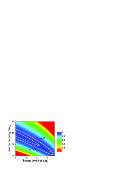
Figure 3:  (color online) Contour plot of the steady-state average phonon number ${n}_{\rm st}$ in the MR as a function of the normalized driving detuning $\Delta/\omega_{m}$ and the normalized interdot coupling $\Omega/\omega_{m}$. The two solid curves correspond to ${n}_{\rm st}=0.05$ and $0.02$. The black dasded line represents $\Omega^{2}=\omega_{m}(\omega_{m}-\Delta)$, under which the MR can be optimally cooled. We have chosen $\Omega_{1}=\Omega_{2}=\Omega/\sqrt{2}$ and typical parameters $\omega_{m}=2\pi\times 100$ MHz, $\Gamma=\omega_{m}$, $Q=10^{5}$, $\eta=0.1$, and $n(\omega_{m})=21$.

The underlying physics of the optimal cooling condition in Eq. (36) can be understood based on the eigenstate basis of the TQD. In the limit $\gamma\ll g\ll\omega_{m}$ considered here, the TQD arrives quickly at the dark state $|-\rangle$. The coupling between the MR and the TQD will excite the TQD to the state $|+\rangle$ most readily when the frequency $\omega_{m}$ of the MR is equal to the transition frequency $(\phi+\Delta)/2$ between the states $|-\rangle$ and $|+\rangle$, i.e., $\omega_{m}=(\phi+\Delta)/2$. This corresponds to the transition $|-,n\rangle\rightarrow|+,n-1\rangle$. The excited electron subsequently tunnels to the right electrode, i.e., $|+,n-1\rangle\rightarrow|0,n-1\rangle$. This whole process extracts an energy quantum from the MR. When this cycle repeats, i.e., $|0,n\rangle\rightarrow|-,n\rangle\rightarrow|+,n-1\rangle\rightarrow|0,n-1\rangle\rightarrow\cdots$, the MR is cooled to the ground state. Here we emphasize that the resonance condition for exciting the TQD from the state $|-\rangle$ to the state $|+\rangle$ via the MR is equivalent to the optimal cooling condition in Eq. (36). An electron can also relax from the dark state $|-\rangle$ to the ground state $|g\rangle$ by releasing energy to the MR. However, this heating process of the MR is strongly suppressed because the frequency of the MR is off-resonant to the transition $|-\rangle\rightarrow|g\rangle$ in the TQD.

Figure 3 displays a contour plot of the steady-state average phonon number of the MR (${n}_{\rm st}$) as a function of the effective interdot coupling $\Omega$ ($=\sqrt{\Omega_{1}^{2}+\Omega_{2}^{2}}$) and the energy detuning $\Delta$. Here we choose $\Delta<0$ and $\Omega>\omega_{m}$ to make sure that $W>0$. For these typical parameters, a small ${n}_{\rm st}<0.05$ is predicted over a wide range of values on the $\Omega-\Delta$ plane. This implies that ground-state cooling of the MR should be experimentally accessible. Furthermore, to estimate the cooling rate $W$, we use typical experimental parameters TF08 ; WeilRevModPhys : $\omega_{m}=2\pi\times 100$ MHz, $\Delta=-2\pi\times 300$ MHz, and $g=2\pi\times 10$ MHz. The interdot couplings are chosen as $\Omega_{1}=\Omega_{2}\simeq 2\pi\times 141$ MHz to fulfill the optimal cooling condition $\Omega^{2}=\omega_{m}(\omega_{m}-\Delta)$. Using Eq. (32), one arrives at a cooling rate $W\approx 2\pi\times 2$ MHz. Considering a MR with a quality factor $Q=10^{5}$ (see, e.g., Ref. Huttel09, ), one has $\gamma=\omega_{m}/Q=2\pi\times 1$kHz. Therefore, appreciable cooling with $W\gg\gamma$ can be achieved. In this case, a MR can be cooled from, e.g., an initial temperature $T=100$ mK corresponding to $n(\omega_{m})=21$ down to $T=0.8$ mK with ${n}_{\rm st}=0.017$.

In contrast, for sideband cooling of a MR Wilson04 ; Wilson07 ; Zippilli09 ; Ouyang09 , the resolved-sideband cooling condition $\omega_{m}\gg\Gamma$ must be followed for ground-state cooling of a MR. For a relatively large decay rate, only MR with a very high frequency (which becomes fragile in experiments) can be cooled. On the other hand, for cooling via quantum interference in the TQD proposed here, the cooling conditions $\Omega^{2}=\omega_{m}(\omega_{m}-\Delta)$ and $\Delta\gg\Gamma$ do not require a high MR frequency.

V A scheme for verifying the cooling of the MR

V.1 Quantum dynamics of coupled MR-DQD system in the presence of a charge detector

To verify whether the MR is cooled or not, we propose a scheme in which the MR is coupled to a two-level system realized by a double quantum dot (DQD). The state of the DQD is in turn measured by a nearby charge detector in the form of, e.g., a quantum point contact (QPC). This setup is schematically shown in Fig. 4. Experimentally, the cooling and the verification setups are all fabricated on the same chip with shared components. Dots 1 and 3 in the TQD from the above cooling setup can make up the DQD after a gate voltage is applied to decouple dot $2$ from dot $3$. Also, the QPC should be decoupled from the rest of the system during cooling by applying a high gate voltage.

The Hamiltonian of the system is given by

$$H=H_{R}+H_{\rm DQD}+H_{\rm QPC}+H_{\rm int}+H_{\rm det}.$$ (38)

The Hamiltonian $H_{R}$ of the MR and the coupling $H_{\rm int}$ between the MR and the DQD are already given in Eqs. (5) and (7). Here $H_{\rm DQD}$, $H_{\rm QPC}$ and $H_{\rm det}$ are respectively the Hamiltonians of the DQD, the QPC and the coupling between them and are given by

$$H_{\rm DQD}\! =\! -\frac{\Delta}{2}\sigma_{z}+\Omega_{1}\sigma_{x},$$

$$H_{\rm QPC}\! =\! \sum_{kq}\omega_{Sk}c_{Sk}^{\dagger}c_{Sk}+\omega_{Dq}c_{Dq}^{\dagger}c_{Dq},$$

$$H_{\rm det}\! =\! \sum_{kq}(T-\chi\sigma_{z})(c_{Sk}^{\dagger}c_{Dq}+{\rm H.c.}),$$ (39)

where $\sigma_{z}=a_{3}^{\dagger}a_{3}-a_{1}^{\dagger}a_{1}$ and $\sigma_{x}=a_{3}^{\dagger}a_{1}+a_{1}^{\dagger}a_{3}$ are the Pauli matrices. Also, $c_{ik}$ ($c_{ik}^{\dagger}$) is the annihilation (creation) operator for an electron with momentum $k$ in either the source ($i=S$) or the drain ($i=D$) of the QPC. $T$ is the transition amplitude of an isolated QPC and $\chi$ is the variation of the transition amplitude caused by the DQD. For simplicity, we assume that the detunning $\Delta$ of the DQD is zero. The DQD has the eigenstates

$$|g\rangle=\frac{\sqrt{2}}{2}(|1\rangle-|3\rangle),~{}~{}|e\rangle=\frac{\sqrt{2}}{2}(|1\rangle+|3\rangle),$$ (40)

with $|g\rangle$ ($|e\rangle$) being the ground (excited) state. Rewriting the Hamiltonian in Eq. (38) on the eigenstate basis of the DQD, we have

$$H\! =\! \omega_{m}b^{\dagger}b+\Omega_{1}\rho_{z}-g\rho_{x}(b^{\dagger}+b)+H_{\rm QPC}$$ (41)

$$+\sum_{kq}(T-\chi\rho_{x})(c_{Sk}^{\dagger}c_{Dq}+{\rm H.c.}),$$

where $\rho_{z}=|e\rangle\langle e|-|g\rangle\langle g|$ and $\rho_{x}=|e\rangle\langle g|+|g\rangle\langle e|$ are the Pauli matrices.

We consider the coupled MR-DQD system in the strong dispersive regime where the coupling strength is much smaller than the difference between the transition frequency $2\Omega_{1}$ of the DQD and that of the MR, i.e., $g\ll\delta=2\Omega_{1}-\omega_{m}$. This regime was previously considered to study whether the vibration of a MR coupled to a superconducting circuit is classical or quantum mechanical Wei06 . In this regime, the phonon in the MR is only virtually exchanged between the DQD and the MR. Thus, the coupling of the DQD to the MR does not change the occupation probability of the electron in the DQD, but only results in phonon-number-dependent Stark shifts on energy levels of the DQD. Moreover, the Stark shifts can be detected by measuring the full-frequency current spectrum of the QPC.

Figure 4:  (color online) Schematic diagram of a MR capacitively coupled to a DQD which is under measurement by a nearby QPC. The energy detuning between the two dot states in the DQD is $\Delta$ and the interdot coupling strength between them is $\Omega_{1}$.

Applying both a rotating-wave approximation and a canonical transformation $U^{\prime}=e^{s^{\prime}}$ with

$$s^{\prime}=\eta(\rho_{-}b^{\dagger}-\rho_{+}b),~{}~{}\eta=g/\delta,$$ (42)

to the Hamiltonian $H$, one obtains [up to $\mathcal{O}(\eta^{2})$]

$$H\! \approx \!\omega_{m}b^{\dagger}b+\frac{2\Omega_{1}+{g^{2}}(2b^{\dagger}b+1)/{\delta}}{2}\rho_{z}$$ (43)

$$+\frac{g^{2}}{2\delta}(|g\rangle\langle g|+|e\rangle\langle e|)+H_{\rm QPC}$$

$$+\sum_{kq}(T-\chi\rho_{x})(c_{Sk}^{\dagger}c_{Dq}+{\rm H.c.}).$$

From Eq. (43), after taking the trace over the degrees of freedom of the QPC, one obtains the following master equation for the reduced density matrix elements of the coupled MR-DQD system Backaction :

$$\dot{\rho}_{gn,gn}\! =\! -\gamma_{+}\rho_{gn,gn}+(\gamma_{-}+\gamma_{d})\rho_{en,en},$$

$$\dot{\rho}_{en,en}\! =\! \gamma_{+}\rho_{gn,gn}-(\gamma_{-}+\gamma_{d})\rho_{en,en},$$

$$\dot{\rho}_{gn,en}\! =\! -i\delta_{n}\rho_{gn,en}-(\gamma_{1}+\frac{\gamma_{d}}{2})\rho_{gn,en},$$ (44)

where $\delta_{n}=2\Omega_{1}+{g^{2}}(2n+1)/\delta$ and $\gamma_{1}=2\pi g_{s}g_{d}\chi^{2}eV_{d}$ with $g_{s}$ ($g_{d}$) being the density of states for electrons in the source (drain) of the QPC and $V_{d}$ the bias voltage across the QPC. Here $\gamma_{\pm}=\gamma_{1}(1\mp\lambda_{n})$, with $\lambda_{n}=\delta_{n}/eV_{d}$, are the QPC-induced excitation and relaxation rates between the ground state and the excited state of the DQD. Also, $\gamma_{d}$ is the relaxation rate resulting from the coupling of the DQD to the thermal bath. Since the dissipation rate of the MR is much smaller than that of the DQD, dissipation of the MR is neglected. In Eq. (44), the reduced density matrix element $\rho_{in,in}$ ($i=g,e$) gives the occupation probability of the state $|i,n\rangle$ of the coupled MR-DQD system ,while $\rho_{in,jn}$ ($i\neq j$) describes the coherence between the states $|i,n\rangle$ and $|j,n\rangle$. The equations of motion for other elements, e.g., $\rho_{in,jn^{\prime}}$ ($n\neq n^{\prime}$), which are decoupled from those considered here, are not shown. Using Eq. (44) and the normalization condition $p_{n}=\rho_{gn,gn}+\rho_{en,en}$, one finds

$$\rho_{gn,gn}(t)\! \!=\! \!\frac{(\gamma_{-}+\gamma_{d})p_{n}}{2\gamma_{0}}$$

$$-\big{[}\frac{(\gamma_{-}+\gamma_{d})p_{n}}{2\gamma_{0}}-\rho_{gn,gn}(0)\big{]}e^{-2\gamma_{0}t},$$

$$\rho_{en,en}(t)\! \!=\! \!\frac{\gamma_{+}}{2\gamma_{0}}p_{n}-\big{[}\frac{\gamma_{+}}{2\gamma_{0}}p_{n}-\rho_{en,en}(0)\big{]}e^{-2\gamma_{0}t},$$

$$\rho_{gn,en}(t)\! \!=\! \!\rho_{gn,en}(0)e^{-i(\delta_{n}-\gamma_{0})t},$$ (45)

where $\gamma_{0}=\gamma_{1}+\gamma_{d}/2$ and $p_{n}$ is the probability that the MR is at state $|n\rangle$.

V.2 Current spectrum of the charge detector

The dc current through the QPC is related to the electron occupation probability in the DQD and is given by GurvitzPRB97

$$I(t)\!=eD\rho_{11}+eD^{\prime}\rho_{33}=\frac{e}{2}(D+D^{\prime})+\frac{e}{2}(D^{\prime}-D)\langle\sigma_{z}\rangle,$$ (46)

where

$$D\! \!=\! \!2\pi g_{s}g_{d}(T-\chi)^{2}V_{d},$$

$$D^{\prime}\! \!=\! \!2\pi g_{s}g_{d}(T+\chi)^{2}V_{d},$$ (47)

are the respective rates of electron tunneling through the QPC when dot $3$ is respectively occupied or empty GurvitzPRB97 . Therefore, one can define the current operator as

$$I(t)=I_{0}+I_{1}\sigma_{z}(t)=I_{0}+I_{1}\rho_{x}(t),$$ (48)

with $I_{0,1}=e(D\pm D^{\prime})/2$. According to the Wiener-Khintchine theorem, the power spectrum of the current through the QPC is Scully

$$S(\omega)\!=\!{\rm Re}\!\!\int\limits_{0}^{\infty}e^{i\omega\tau}d\tau[\langle I(t)I(t+\tau)\rangle-\langle I(t+\tau\rangle\langle I(t)\rangle].$$ (49)

Substituting Eqs. (45) and (48) into Eq. (49), we get

$$S(\omega)/S_{0}\! \!=\! \!1+\frac{2\gamma_{1}\gamma_{2}}{\gamma_{1}+\gamma_{2}}\sum_{n}p_{n}(1-\kappa p_{n})\frac{\gamma_{0}}{\gamma_{0}^{2}+(\delta_{n}-\omega)^{2}}$$

$$-\frac{2\gamma_{1}\gamma_{2}}{\gamma_{1}+\gamma_{2}}\sum_{n}p_{n}(1+\kappa p_{n})\frac{\gamma_{0}}{\gamma_{0}^{2}+(\delta_{n}+\omega)^{2}},$$

where $\gamma_{2}=2\pi g_{s}g_{d}T^{2}V_{d}$, $\kappa=(\gamma_{+}-\gamma_{-}-\gamma_{d})/2\gamma_{0}$, and $S_{0}=2eI_{0}$ is the current-noise background. From Eq. (LABEL:spectrum), one sees that the current spectrum of the QPC consists of peaks at resonance points $\omega=\pm\delta_{n}$. These peaks have width $\gamma_{0}$ and heights increasing with the probability $p_{n}$. For instance, the peaks at the resonance point

$$\delta_{n}=2\Omega_{1}+\frac{g^{2}(2n+1)}{\delta},$$ (51)

is shifted by ${g^{2}}(2n+1)/\delta$ from $2\Omega_{1}$. Thus, from this peak shift in the current spectrum, one can readout the phonon-number state of the MR.

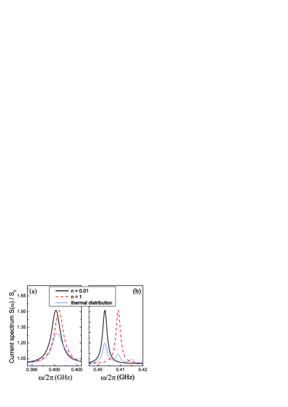
Figure 5:  (color online) Power spectrum of the current through the QPC when the phonon number in the MR are respectively $n=0.01$ (black solid line), $n=1$ (red dashed line), or given by the thermal distribution (blue dotted line), i.e., $p_{n}={n}_{\rm st}^{n}/{(1+{n}_{\rm st})^{n+1}}$ with ${n}_{\rm st}=1$. The coupling strength between the MR and the DQD is $g=0.1~{}\omega_{m}$ (a) and $g=0.3~{}\omega_{m}$ (b). The other parameters are $\omega_{m}=100~{}$MHz, $\Omega_{1}=2\omega_{m}$, $\gamma_{2}=0.01\omega_{m}$, $\gamma_{1}=0.2\gamma_{2}$, and $\gamma_{d}=2\gamma_{2}$.

Figure 4 plots the current spectrum of the QPC with two different coupling strengths between the MR and the DQD. Results for three cases in which the MR is respectively in its ground state ($n=0.01\ll 1$), the first-excited state ($n=1.0$) or thermalized with an average phonon number ${n}_{\rm st}=1.0$ are plotted. Each resonance peak in the current spectrum corresponds to a phonon-number state of the MR. For the thermally distributed case, the current spectrum shows several peaks, where the relative area under each peak gives the probability of the corresponding phonon-number state. As shown in Fig. 4(a), the distance between two adjacent peaks is smaller than the intrinsic peak width in the weak dispersive regime, i.e., $2g^{2}/\delta<\gamma_{0}$, and hence the measured spectrum shows an ensemble. In this case, the phonon-number state of the MR cannot be measured. In the strong limit ($2g^{2}/\delta>\gamma_{0}$), however, the ensemble can be individually resolved [Fig. 4(b)], which allows us to detect the phonon number and also to verify the cooling result of the MR. Indeed, a relatively strong coupling between a MR and a quantum dot has been recently demonstrated Huttel09 . The strong dispersive regime is thus achievable and one can apply the proposed coupled MR-DQD system to verify the cooling of the MR via measuring the current spectrum of a nearby charge detector (e.g., QPC).

VI Discussion and Conclusion

Our proposal on ground state cooling of the MR requires that the TQD is able to evolve into the dark state. However, the dephasing of the TQD due to coupling to other degrees of freedom in the environment can project the TQD into one of the three localized states $|1\rangle$, $|2\rangle$, and $|3\rangle$ and drive the system away from the dark state Michaelis06 . However, the dephasing between the two localized states $|1\rangle$ and $|2\rangle$ depends on the coupling strength and the energy detunning between dots $1$ and $2$ BrandesPRL00 . Here in our system no direct coupling exists between the two localized states $|1\rangle$ and $|2\rangle$, and thus the dephasing almost has negligible effects on the cooling efficiency of the MR.

In summary, we have studied the cooling of a MR by capacitive coupling to a TQD. We show that when the two lower-energy localized states become degenerate, the TQD will be trapped in a dark state which is decoupled from the excited state in the absence of the MR. With the MR in resonance with the transition between the dark state and the excited eigenstate in the TQD, we have shown that the MR can be cooled to its ground state in the non-resolved sideband cooling regime. Moreover, we have proposed a coupled MR-DQD system in the strong dispersive regime for verifying the cooling result of the MR. In this regime, the coupling between the MR and the DQD induces a MR-phonon-number dependent shift of the transition frequency of the DQD. Thus the phonon-number state which characterizes the cooling result of the MR can be detected by measuring the shifts of the resonance peaks in the current spectrum of a nearby charge detector.

Appendix A Master equation for the reduced density matrix of the MR

In this appendix, we derive the master equation [Eq. (28)] for the reduced density matrix of the MR from the master equation [Eq. (24)] of the coupled MR-TQD system by eliminating the degrees of freedom of the TQD. In general, the dissipation rate of the MR is much smaller than the decay rate of the TQD, i.e., $[n(\omega_{m})+1]\gamma\ll\Gamma$. The TQD hence attains its steady-state quickly and its perturbation to the MR can be regarded as part of the environment Wilson07 ; Cirac92 . Up to the second order in $\eta$, Eq. (24) can be rewritten as

$$\frac{d\rho}{dt}\!=\!\mathcal{L}\rho=[\mathcal{L}_{0}+\mathcal{L}_{1}+\mathcal{L}_{2}]\rho,$$ (52)

where

$$\mathcal{L}_{0}{\rho}\! =\! -i\omega_{m}[b^{\dagger}b,\,\rho]-i[H_{\rm TQD},\rho]$$ (53)

$$+\Gamma_{1}\mathcal{D}[a_{1}^{\dagger}]\rho+\Gamma_{2}\mathcal{D}[a_{2}^{\dagger}]\rho+\Gamma_{3}\mathcal{D}[a_{3}]\rho,$$

$$\mathcal{L}_{1}\rho\! =\! -i[V(b^{\dagger}-b),\rho],$$ (54)

$$\mathcal{L}_{2}\rho\! =\! \eta^{2}\Gamma_{1}(\mathcal{D}[a_{1}^{\dagger}b^{\dagger}]\rho+\mathcal{D}[a_{1}^{\dagger}b]\rho)$$ (55)

$$+\eta^{2}\Gamma_{3}(\mathcal{D}[a_{3}b^{\dagger}]\rho+\mathcal{D}[a_{3}b]\rho)+\mathcal{L}_{\rm D}\rho,$$

are respectively the Liouvillians to zeroth, first, and second orders in $\eta$. At zeroth order in $\eta$, the quantum dynamics of the whole system is described by

$$\dot{\rho}(t)=\mathcal{L}_{0}\rho(t).$$ (56)

The MR and the TQD are decoupled. Since the TQD is at its steady state most of the time, one has $\rho(t)=\rho_{d}^{\rm st}\otimes{\rm Tr}_{d}\{\rho\}$ with $\rho_{d}^{\rm st}$ denoting the reduced density matrix of the TQD at steady-state and ${\rm Tr}_{d}\{\cdots\}$ the trace over the TQD’s degrees of freedom. Equation (56) has an infinite number of steady-state solutions. These solutions can be expanded in the basis of the eigenvectors $\rho_{d}^{\rm st}\otimes|n\rangle\langle n^{\prime}|$ of the Liouville operator $\mathcal{L}_{0}$ with eigenvalues $\lambda_{nn^{\prime}}=-i(n-n^{\prime})\omega_{m}$, i.e., $\mathcal{L}_{0}\rho_{nn^{\prime}}=\lambda_{nn^{\prime}}\rho_{nn^{\prime}}$ Morigi00 . Here, $|n\rangle$ ($n=0,1,2,\cdots$) denotes the $n$th state of the MR and $(n-n^{\prime})\omega_{m}$ represents the energy difference between the states $|n\rangle$ and $|n^{\prime}\rangle$. For $\eta\neq 0$, these states with different $n$ are weakly coupled by the perturbative terms $\mathcal{L}_{1}$ and $\mathcal{L}_{2}$. To obtain the quantum dynamics of the MR, we project the system onto the subspace with a zero eigenvalue ($n=n^{\prime}$) of $\mathcal{L}_{0}$. The projection operator $\mathcal{P}$ is defined by

$$\mathcal{L}_{0}\mathcal{P}\rho=0.$$ (57)

Noting $g\ll\omega_{m}$ (i.e., $\eta\ll 1$), a second order perturbation expansion gives the following closed equation for $\mathcal{P}\rho$  Ouyang09

$$\mathcal{P}\dot{\rho}(t)=\mathcal{P}\mathcal{L}_{2}\mathcal{P}\rho(t)+\int\limits_{0}^{\infty}d\tau\mathcal{P}\mathcal{L}_{1}e^{\mathcal{L}_{0}\tau}\mathcal{L}_{1}\mathcal{P}\rho(t).$$ (58)

Substituting Eqs. (54) and (55) into Eq. (58) and taking the trace over the TQD degrees of freedom, the first term in Eq. (58) becomes Cirac92

$${\rm Tr}_{d}\{\mathcal{P}\mathcal{L}_{2}\mathcal{P}\rho(t)\}\! \!=\! \!\frac{1}{2}[\gamma n(\omega_{m})+\eta^{2}\Gamma_{1}\rho_{00}^{\rm st}]\mathcal{D}[b]\mu$$

$$+\frac{1}{2}\big{\{}\gamma[n(\omega_{m})+1]+\eta^{2}\Gamma_{1}\rho_{00}^{\rm st}\big{\}}\mathcal{D}[b^{\dagger}]\mu,$$

and the second term gives

$${\rm Tr}_{d}\bigg{\{}\int\limits_{0}^{\infty}d\tau\mathcal{P}\mathcal{L}_{1}e^{\mathcal{L}_{0}\tau}\mathcal{L}_{1}\mathcal{P}\rho(t)\bigg{\}}$$ (60)

$$\!=\! \!-i(\omega_{m}+\delta_{m})[b^{\dagger}b,\mu],$$

$$+{\rm Re}[G(i\omega_{m})]\mathcal{D}[b]\mu+{\rm Re}[G(-i\omega_{m})]\mathcal{D}[b^{\dagger}]\mu,$$

where $\mu={\rm Tr}_{d}\{\mathcal{P}\rho\}$ is the reduced density matrix of the MR and $\rho_{00}^{\rm st}$ is the probability of an empty TQD at the steady state. Here, we have defined

$$\delta_{m}={\rm Im}[G(i\omega_{m})+G(-i\omega_{m})].$$ (61)

Thus, from Eqs. (58), (LABEL:firstterm) and (60), one has

$$\dot{\mu} = -i(\omega_{m}+\delta_{m})[b^{\dagger}b,\mu]+\frac{1}{2}[\gamma n(\omega_{m})+A_{+}]\mathcal{D}[b]\mu$$ (62)

$$+\frac{1}{2}\big{\{}\gamma[n(\omega_{m})+1]+A_{-}\big{\}}\mathcal{D}[b^{\dagger}]\mu,$$

where

$$A_{\pm}=2\,{\rm Re}[G(\pm i\omega_{m})]+\eta^{2}\Gamma_{1}\rho_{00}^{\rm st}.$$ (63)

Eq. (62) is simply the master equation (28) for the reduced density matrix of the MR derived in Sec. IV. In Eq. (60), the correlation function $G(s)$ is given by

$$G(s)\! \!=\! \!-{\rm Tr}_{d}\int\limits_{0}^{\infty}dtV(0)e^{\mathcal{L}_{\rm TQD}t}V(0)e^{st}$$ (64)

$$\!=\! \!-\int\limits_{0}^{\infty}d\tau\langle V(t)V(0)\rangle e^{st}\!=\!-\langle\widetilde{V}(s)V(0)\rangle,$$

where $s=i\omega_{m}$. Also, $\widetilde{V}(s)$ is the Laplace transform of $V(t)$ and the Liouvillians $\mathcal{L}_{\rm TQD}$ is given in Eq. (LABEL:ME-TQD).

To determine the correlation function $G(\pm s)$, one first calculate the Laplace transform $\widetilde{V}(s)$ of the interaction term $V(t)$. For convenience, we introduce the vector operator $\hat{\sigma}$ for the TQD whose components are defined as

$$\hat{\sigma}_{1}=|1\rangle\langle 1|,~{}\hat{\sigma}_{2}=|2\rangle\langle 2|,~{}\hat{\sigma}_{3}=|3\rangle\langle 3|,$$

$$\hat{\sigma}_{4}=|1\rangle\langle 2|,~{}\hat{\sigma}_{5}=|2\rangle\langle 1|,~{}\hat{\sigma}_{6}=|1\rangle\langle 3|,$$

$$\hat{\sigma}_{7}=|3\rangle\langle 1|,~{}\hat{\sigma}_{8}=|2\rangle\langle 3|,~{}\hat{\sigma}_{9}=|3\rangle\langle 2|,$$ (65)

where the average value of each component is $\langle\hat{\sigma}_{i}\rangle={\rm Tr}\{\hat{\sigma}_{i}\rho_{d}\}$. Using this notation, one has

$$V=2\eta\Omega_{1}(\hat{\sigma}_{7}-\hat{\sigma}_{6})+\eta\Omega_{2}(\hat{\sigma}_{9}-\hat{\sigma}_{8}).$$ (66)

and thus

$$G(s)\! \!=\! \!-2\eta\Omega_{1}[S_{7}(s)-S_{6}(s)]-\eta\Omega_{2}[S_{9}(s)-S_{8}(s)],$$

where $S_{i}(s)=\langle\widetilde{\sigma}_{i}(s)V(0)\rangle$ with $\langle\widetilde{\sigma}_{i}(s)\rangle$ being the Laplace transform of $\langle\hat{\sigma}_{i}(t)\rangle$. From Eq. (LABEL:ME-TQD), we find that $\langle\hat{\sigma}_{i}(t)\rangle$ obeys the equation of motion:

$$\frac{d{\langle\hat{\sigma}(t)\rangle}}{dt}=M{\langle\hat{\sigma}(t)\rangle}+B,$$ (68)

where

$$\begin{array}[]{l}M\!=\!\left({\begin{array}[]{*{20}c}-\Gamma_{1}&-\Gamma_{1}&-\Gamma_{1}&0&0&-i\Omega_{1}&i\Omega_{1}&0&0\\ -\Gamma_{2}&-\Gamma_{2}&-\Gamma_{2}&0&0&0&0&-i\Omega_{2}&i\Omega_{2}\\ 0&0&-\Gamma_{3}&0&0&i\Omega_{1}&-i\Omega_{1}&i\Omega_{2}&-i\Omega_{2}\\ 0&0&0&-i\Delta_{d}&0&-i\Omega_{2}&0&0&i\Omega_{1}\\ 0&0&0&0&i\Delta_{d}&0&i\Omega_{2}&-i\Omega_{1}&0\\ -i\Omega_{1}&0&i\Omega_{1}&-i\Omega_{2}&0&\lambda_{1}&0&0&0\\ i\Omega_{1}&0&-i\Omega_{1}&0&i\Omega_{2}&0&\lambda_{1}^{*}&0&0\\ 0&-i\Omega_{2}&i\Omega_{2}&0&-i\Omega_{1}&0&0&\lambda_{2}&0\\ 0&i\Omega_{2}&-i\Omega_{2}&i\Omega_{1}&0&0&0&0&\lambda_{2}^{*}\\ \end{array}}\right),\\ \end{array}$$ (79)

and $B=(\Gamma_{1},\Gamma_{2},0,0,0,0,0,0,0)^{T}$. Here we have defined $\Delta_{d}\equiv\Delta_{1}-\Delta_{2}$, $\lambda_{1}\equiv-(i\Delta_{1}+\frac{1}{2}\Gamma_{3})$, and $\lambda_{2}\equiv-(i\Delta_{2}+\frac{1}{2}\Gamma_{3})$. From Eq. (68), the steady-state solution of the vector $\langle\hat{\sigma}\rangle$ is calculated as

$$\langle\hat{\sigma}^{\rm st}\rangle=M^{-1}B.$$ (81)

Applying the Laplace transform to Eq. (68), one obtains

$$s\langle\widetilde{{\sigma}}(s)\rangle-\langle\hat{\sigma}(0)\rangle=M\langle\widetilde{{\sigma}}(s)\rangle+\frac{B}{s}.$$ (82)

Moreover, the $i$th component of the vector $\langle\widetilde{\sigma}(s)\rangle$ is given by

$$\langle\widetilde{{\sigma}}_{i}(s)\rangle=\sum_{k=1}^{9}L_{ik}[\langle\hat{\sigma}_{k}(0)\rangle+\frac{B_{k}}{s}].$$ (83)

Here the matrix $L$ is defined as $L=(sI-M)^{-1}$ where $I$ denotes the identity matrix. Assuming that the TQD has already attained its steady-state at initial time $t=0$, i.e., $\langle\hat{\sigma}(0)\rangle=\langle\hat{\sigma}^{\rm st}\rangle$, using Eqs. (66), (A), (81), (83) and the quantum regression theorem Scully , one can obtain the correlation function $G(s)$ and the scattering rates $A_{\pm}$ as given in Eq. (63).

References

• (1) K. C. Schwab and M. L. Roukes, Phys. Today 58, 36 (2005).
• (2) X. M. H. Huang, C. A. Zorman, M. Mehregany, and M. L. Roukes, Nature (London) 421, 496 (2003).
• (3) M. D. LaHaye, O. Buu, B. Camarota, and K. C. Schwab, Science 304, 74 (2004).
• (4) V. Braginsky and S. P. Vyatchanin, Phys. Lett. A 293, 228 (2002).
• (5) E. Buks and B. Yurke, Phys. Rev. E 74, 046619 (2006).
• (6) S. Savel’ev, X. Hu, and F. Nori, New J. Phys. 8, 105 (2006).
• (7) S. Savel’ev, A. L. Rakhmanov, X. Hu, A. Kasumov, and F. Nori, Phys. Rev. B 75, 165417 (2007).
• (8) D. Vitali, S. Gigan, A. Ferreira, H. R. Böhm, P. Tombesi, A. Guerreiro, V. Vedral, A. Zeilinger, and M. Aspelmeyer, Phys. Rev. Lett. 98, 030405 (2007).
• (9) M. J. Hartmann and M. B. Plenio, Phys. Rev. Lett. 101, 200503 (2008).
• (10) L. Tian and P. Zoller, Phys. Rev. Lett. 93, 266403 (2004).
• (11) T. F. Li, Yu. A. Pashkin, O. Astafiev, Y. Nakamura, J. S. Tsai, and H. Im, Appl. Phys. Lett. 92, 043112 (2008).
• (12) A. K. Hüttel, G. A. Steele, B. Witkamp, M. Poot, L. P. Kouwenhoven, and H. S. J. van der Zant, Nano Lett. 9, 2547 (2009).
• (13) C. H. Metzger and K. Karrai, Nature (London) 432, 1002 (2004).
• (14) S. Gigan, H. R. Bohm, M. Paternostro, F. Blaster, G. Langer, J. B. Hertzberg, K. C. Schwab, D. Bauerle, M. Aspelmeyer, and A. Zeilinger, Nature (London) 444, 67 (2006).
• (15) D. Kleckner and D. Bouwmeester, Nature (London) 444, 75 (2006).
• (16) O. Arcizet, R. F. Cohadon, T. Briant, M. Pinard, and A. Heidmann, Nature (London) 444, 71 (2006).
• (17) A. Naik, O. Buu, M. D. LaHaye, A. D. Armour, A. A. Clerk, M. P. Blencowe, and K. C. Schwab, Nature (London) 443, 193 (2006).
• (18) A. Schliesser, P. Del’Haye, N. Nooshi, K. J. Vahala, and T. J. Kippenberg, Phys. Rev. Lett. 97, 243905 (2006).
• (19) M. Poggio, C. L. Degen, H. J. Mamin, and D. Rugar, Phys. Rev. Lett. 99, 017201 (2007).
• (20) J. D. Teufel, C. A. Regal, and K. W. Lehnert, New J. Phys. 10, 095002 (2008).
• (21) T. J. Kippenberg, H. Rokhsari, T. Carmon, A. Scherer, and K. J. Vahala, Phys. Rev. Lett. 95, 033901 (2005).
• (22) P. Zhang, Y. D. Wang, and C. P. Sun, Phys. Rev. Lett. 95, 097204 (2005); Y.D. Wang, Y. Li, F. Xue, C. Bruder, and K. Semba, Phys. Rev. B 80, 144508 (2009).
• (23) J. Q. You, Y. X. Liu, and F. Nori, Phys. Rev. Lett. 100, 047001 (2008).
• (24) I. Wilson-Rae, P. Zoller, and A. Imamoglu, Phys. Rev. Lett. 92, 075507 (2004).
• (25) S. H. Ouyang, J. Q. You, and F. Nori, Phys. Rev. B 79, 075304 (2009).
• (26) S. Zippilli, G. Morigi, and A. Bachtold, Phys. Rev. Lett. 102, 096804 (2009).
• (27) I. Wilson-Rae, N. Nooshi, W. Zwerger, and T. J. Kippenberg, Phys. Rev. Lett. 99, 093901 (2007); I. Wilson-Rae, N. Nooshi, J. Dobrindt, T. J. Kippenberg, and W. Zwerger, New J. Phys. 10, 095007 (2008).
• (28) F. Marquardt, J. P. Chen, A. A. Clerk, and S. M. Girvin, Phys. Rev. Lett. 99, 093902 (2007).
• (29) A. Schliesser, R. Riviére, G. Anetsberger, O. Arcizet, and T. J. Kippenberg, Nature Phys. 4, 415 (2008).
• (30) Y. Li, Y. D Wang, F. Xue, and C. Bruder, Phys. Rev. B 78, 134301 (2008).
• (31) M. Grajcar, S. Ashhab, J. R. Johansson, and F. Nori, Phys. Rev. B 78, 035406 (2008).
• (32) See, e.g., J. Q. You and F. Nori, Phys. Today 58, No. 11, 42 (2005).
• (33) G. Morigi, J. Eschner, and C. H. Keitel, Phys. Rev. Lett. 85, 4458 (2000); G. Morigi, Phys. Rev. A 67, 033402 (2003).
• (34) M. O. Scully and M. S. Zubairy, Quantum Optics (Cambridge University Press, Cambridge, 1997), Chapt. 10.
• (35) K. Xia and J. Evers, Phys. Rev. Lett. 103, 227203 (2009).
• (36) D. T. McClure, L. DiCarlo, Y. Zhang, H.-A. Engel, C. M. Marcus, M. P. Hanson and A. C. Gossard, Phys. Rev. Lett. 98, 056801 (2007).
• (37) N. Lambert, and F. Nori, Phys. Rev. B 78, 214302 (2008).
• (38) B. Michaelis, C. Emary, and C. W. J. Beenakker, EuroPhys. Lett. 63, 677 (2006); C. Emary, Phys. Rev. B 76, 245319 (2007).
• (39) J. I. Cirac, R. Blatt, P. Zoller and W. D. Phillips, Phys. Rev. A 46, 2668 (1992).
• (40) W. G. van der Wiel, S. De Franceschi, J. M. Elzerman, T. Fujisawa, S. Tarucha, and L. P. Kouwenhoven, Rev. Mod. Phys. 75, 1 (2002).
• (41) L. F. Wei, Y.X. Liu, C. P. Sun, and Franco Nori, Phys. Rev. Lett. 97, 237201 (2006).
• (42) S. H. Ouyang, C. H. Lam, and J. Q. You, arXiv:0910.5052 (unpublised).
• (43) S. A. Gurvitz, Phys. Rev. B 56, 15215 (1997).
• (44) T. Brandes, and F. Renzoni, Phys. Rev. Lett. 85, 4148 (2000).