Domain walls of ferroelectric BaTiO₃ within the Ginzburg-Landau-Devonshire phenomenological model

Abstract

Mechanically compatible and electrically neutral domain walls in tetragonal, orthorhombic and rhombohedral ferroelectric phases of BaTiO₃ are systematically investigated in the framework of the phenomenological Ginzburg-Landau-Devonshire (GLD) model with parameters of Ref. [Hlinka and Marton, Phys. Rev. 74, 104104 (2006)]. Polarization and strain profiles within domain walls are calculated numerically and within an approximation leading to the quasi-one-dimensional analytic solutions applied previously to the ferroelectric walls of the tetragonal phase [W. Cao and L.E. Cross, Phys. Rev. 44, 5 (1991)]. Domain wall thicknesses and energy densities are estimated for all mechanically compatible and electrically neutral domain wall species in the entire temperature range of ferroelectric phases. The model suggests that the lowest energy walls in the orthorhombic phase of BaTiO₃ are the 90-degree and 60-degree walls. In the rhombohedral phase, the lowest energy walls are the 71-degree and 109-degree walls. All these ferroelastic walls have thickness below 1 nm except for the 90-degree wall in the tetragonal phase and the 60-degree S-wall in the orthorhombic phase, for which the larger thickness of the order of 5 nm was found. The antiparallel walls of the rhombohedral phase have the largest energy and thus they are unlikely to occur. The calculation indicates that the lowest energy structure of the 109-degree wall and few other domain walls in the orthorhombic and rhombohedral phases resemble Bloch-like walls known from magnetism.

I INTRODUCTION

Domain structure is an important ingredient in functionality of ferroelectric materials. Among others, it has impact on their nonlinear optical properties, dielectric permittivity and polarization switching phenomena. Since domain boundaries in ferroelectric perovskite materials can simultaneously play the role of the ferroelectric and ferroelastic walls, such domain walls also strongly influence the electromechanical material properties: they facilitate switching of spontaneous polarization and spontaneous deformation, thus giving rise to a large extrinsic contribution to e.g. piezoelectric constants, which makes ferroelectric materials extremely attractive for applications. The domain structure also provides additional degree of freedom for tuning of material properties. In general, further development of domain engineering strategies requires deeper understanding of the physics of ferroelectric domain wall itself.

The Ginzburg-Landau-Devonshire (GLD) theory provides a feasible tool for such a purpose. Landau-Devonshire model describes phase-transition properties of single-domain crystal using a limited number of parameters, which are determined experimentally (or recently also using ab-initio methods). Introduction of Ginzburg gradient term to the free energy functional enables addressing nonhomogeneous multi-domain ferroelectric state. The GLD model was previously used for computation of domain wall properties in ferroelectric materials (e.g. Refs. art_cao_cross_prb_1991, ; art_ishibashi_salje_2002, ; art_huang_jiang_hu_liu_JPCM_1996, ; art_hlinka_marton_prb_2006, ; art_erhart_cao_fousek_ferroelectrics_2001, ) and in phase-field computer modeling of domain formation and evolution.art_nambu_sagala_1994 ; art_hu_chen_1998 ; art_ahluwalia_2003 ; art_marton_hlinka_2006 The GLD model can be regarded as a bridge model covering length-scales inaccessible by ab-initio and micro-mechanical models.

BaTiO₃ represents a typical ferroelectric material which undergoes a sequence of phase transitions from high-temperature paraelectric cubic $Pm3m$ ($O_{h}$) to the ferroelectric tetragonal $P4mm$ ($C_{4v}$), orthorhombic $Amm2$ ($C_{2v}$) and rhombohedral $R3m$ ($C_{3v}$) phase. Energetically equivalent directions of spontaneous polarization vector, identifying possible ferroelectric domain states in a particular ferroelectric phase, are displayed in Fig. 1. Domain boundaries separating two domain states are characterized by the rotational angle needed to match spontaneous polarizations on both sides of the boundary. For example, the boundary separating domains with mutually perpendicular spontaneous polarization is commonly called 90^∘ wall, while the one between antiparallel spontaneous polarization regions is called 180^∘ wall. Other angles are possible in orthorhombic and rhombohedral phases of BaTiO₃, where the spontaneous polarization is oriented along the cubic face diagonals and body diagonals, respectively.

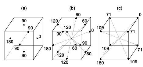
Figure 1: Directions of spontaneous polarization in the (a) tetragonal, (b) orthorhombic and (c) rhombohedral phase. Angles between polarization direction ’0’ and its symmetry equivalent ones are indicated.

The aim of this paper is to calculate basic characteristics of all electrically neutral and mechanically compatible domain walls in all ferroelectric phases of BaTiO₃. For a better comparison of domain wall properties like their thickness or energy density, we employ an Ising-like approximation leading to previously proposed analytically solvable one-dimensional solutions.art_cao_cross_prb_1991 The paper is organized as follows. In Section II. we give an overview of the different kinds of mechanically compatible domain walls in the three ferroelectric phases. It follows from general theory about macroscopic mechanical compatibility of adjacent domain states.art_fousek_janovec_jap_1969 ; janovecIT The GLD parameters used for calculation of the domain wall properties in BaTiO₃ are the same as in our preceding work,art_hlinka_marton_prb_2006 but for the sake of convenience, the definition and the GLD model and its parameters are resumed in Section III. Section IV. is devoted to the description of the computational scheme and approximations applied here to solve analytically the Euler-Lagrange equations. The main result of our study - systematic numerical evaluation of thicknesses, energies, polarization profiles and other properties for different domain walls, is presented in Section V. Sections VI. and VII. are devoted to the discussion of validity of used approximations and the final conclusion, respectively.

II MECHANICALLY COMPATIBLE DOMAIN WALLS IN BARIUM TITANATE

The energy-degeneracy of different directions of spontaneous polarization leads to the appearance of ferroelectric domain structure. Individual domains are separated by domain walls, where the polarization changes from one state to another. Here, only planar domain walls are considered. Orientations of mechanically compatible domain walls are determined by the equation for mechanically compatible interfaces separating two domains with the strain tensors $e_{ij}(-\infty)$ and $e_{ij}(\infty)$ :

$$\sum_{m,n=1}^{3}[e_{mn}(\infty)-e_{mn}(-\infty)]x_{m}x_{n}=0~{}.$$ (1)

Systematic analysis of this equation using symmetry arguments has been done e.g. in Refs. art_fousek_janovec_jap_1969, ; art_fousek_czp_1971, ; janovecIT, . In general, the number $N$ of mechanically compatible domain walls separating two particular domain states can have only one of the three values: $N=0$, $N=2$ or $N=\infty$. In case of $N=2$ there exist two mutually perpendicular domain walls. Each of them is either a crystallographic ($W_{f}$-type) wall or non-crystallographic ($S$-type) wall. Orientation of the $W_{f}$-wall is fixed by symmetry of the crystal, while orientation of the $S$-wall is determined by components of the strain tensor in adjacent domains (and its orientation can be therefore dependent on temperature). For $N=\infty$ there exists infinite number of wall orientations, some of them may be preferred energetically.

Figure 2: Set of mechanically compatible and electrically neutral domain walls in the three ferroelectric phases of BaTiO₃. In the case of 180^∘ domain walls, where the orientation is not determined by symmetry, walls with the most important crystallographic orientations are displayed.

Further, the electrically neutral domain walls will be considered.art_fousek_janovec_jap_1969 It implies that the difference ${\bf P}(\infty)-{\bf P}(-\infty)$ between the spontaneous polarizations in the adjacent domains is perpendicular to the unit vector ${\bf s}$, normal to the domain wall:

$$\left({\bf P}(\infty)-{\bf P}(-\infty)\right)\cdot{\bf s}=0\,.$$ (2)

We also define a unit vector ${\bf r}\parallel({\bf P}(\infty)-{\bf P}(-\infty))$, which identifies the component of the spontaneous polarization which reverses when crossing the wall. Then the charge neutrality condition (2) can be expressed as ${\bf r}\cdot{\bf s}=0$. Finally, let us introduce a third base vector ${\bf t}={\bf r}\times{\bf s}$, which complements the symmetry-adapted orthonormal coordinate system (r, s, t).

BaTiO₃ symmetry allows a variety of domain walls.art_fousek_czp_1971 Ferroelectric walls of BaTiO₃ can be divided in two groups - the non-ferroelasticjanovecIT walls separating domains with antiparallel polarization ($e_{mn}(\infty)-e_{mn}(-\infty)=0$, $N=\infty$) and the ferroelastic walls with other than 180^∘ between polarization in the adjacent domain states ($N=2$). The ${\bf r}\cdot{\bf s}=0$ condition implies that the neutral non-ferroelastic walls are parallel to the spontaneous polarization, and the neutral ferroelastic walls realize a ”head-to-tail” junction. The set of plausible neutral and mechanically compatible domain wall types are schematically shown in Fig. 2. Domain walls are labeled by a symbol composed of the letter specifying the ferroelectric phase (T, O or R staying for the tetragonal, orthorhombic or rhombohedral, resp.), number indicating the polarization rotation angle (180, 120, 109, 90, 71 or 60 degrees) and, if needed, the orientation of the domain wall normal with respect to the parent pseudo-cubic reference structure.

Table 1: Cartesian components of switching vectors ${\bf r}$, domain wall normals ${\bf s}$, and boundary conditions for polarization and strain in adjacent domain states for the inspected domain walls. Vector ${\bf s}_{\rm O60}$ is defined in Eqn. (3), $P_{0}$ stands for magnitude of spontaneous polarization. As usual, spontaneous quantities are those minimizing GLD functional. Numerical values used in this work are given in Sec˙V.

Wall	r	s	${{\bf P}(-\infty)}/{P_{0}}$	${{\bf P}(\infty)}/{P_{0}}$	${\bf e}(-\infty)$	${\bf e}(\infty)$
T180{001}	$(1,0,0)$	$(0,0,1)$	$(1,0,0)$	$(-1,0,0)$	$(e_{\parallel},e_{\perp},e_{\perp},0,0,0)$	$(e_{\parallel},e_{\perp},e_{\perp},0,0,0)$
T180{011}	$(1,0,0)$	$(0,\frac{1}{\sqrt{2}},\frac{1}{\sqrt{2}})$	$(1,0,0)$	$(-1,0,0)$	$(e_{\parallel},e_{\perp},e_{\perp},0,0,0)$	$(e_{\parallel},e_{\perp},e_{\perp},0,0,0)$
T90	$(\frac{1}{\sqrt{2}},\frac{1}{\sqrt{2}},0)$	$(\frac{1}{\sqrt{2}},\frac{-1}{\sqrt{2}},0)$	$(1,0,0)$	$(0,-1,0)$	$(e_{\parallel},e_{\perp},e_{\perp},0,0,0)$	$(e_{\perp},e_{\parallel},e_{\perp},0,0,0)$
O180{1$\bar{1}$0}	$(\frac{1}{\sqrt{2}},\frac{1}{\sqrt{2}},0)$	$(\frac{1}{\sqrt{2}},\frac{-1}{\sqrt{2}},0)$	$(\frac{1}{\sqrt{2}},\frac{1}{\sqrt{2}},0)$	$(\frac{-1}{\sqrt{2}},\frac{-1}{\sqrt{2}},0)$	$(e_{\rm a},e_{\rm a},e_{\rm c},0,0,2e_{\rm b})$	$(e_{\rm a},e_{\rm a},e_{\rm c},0,0,2e_{\rm b})$
O180{001}	$(\frac{1}{\sqrt{2}},\frac{1}{\sqrt{2}},0)$	$(0,0,1)$	$(\frac{1}{\sqrt{2}},\frac{1}{\sqrt{2}},0)$	$(\frac{-1}{\sqrt{2}},\frac{-1}{\sqrt{2}},0)$	$(e_{\rm a},e_{\rm a},e_{\rm c},0,0,2e_{\rm b})$	$(e_{\rm a},e_{\rm a},e_{\rm c},0,0,2e_{\rm b})$
O90	$(0,1,0)$	$(1,0,0)$	$(\frac{1}{\sqrt{2}},\frac{1}{\sqrt{2}},0)$	$(\frac{1}{\sqrt{2}},\frac{-1}{\sqrt{2}},0)$	$(e_{\rm a},e_{\rm a},e_{\rm c},0,0,2e_{\rm b})$	$(e_{\rm a},e_{\rm a},e_{\rm c},0,0,-2e_{\rm b})$
O60	$(\frac{1}{\sqrt{2}},0,\frac{1}{\sqrt{2}})$	${\bf s}_{\rm O60}$	$(\frac{1}{\sqrt{2}},\frac{1}{\sqrt{2}},0)$	$(0,\frac{1}{\sqrt{2}},\frac{-1}{\sqrt{2}})$	$(e_{\rm a},e_{\rm a},e_{\rm c},0,0,2e_{\rm b})$	$(e_{\rm c},e_{\rm a},e_{\rm a},-2e_{\rm b},0,0)$
O120	$(\frac{1}{\sqrt{6}},\frac{2}{\sqrt{6}},\frac{-1}{\sqrt{6}})$	$(\frac{1}{\sqrt{2}},0,\frac{1}{\sqrt{2}})$	$(\frac{1}{\sqrt{2}},\frac{1}{\sqrt{2}},0)$	$(0,\frac{-1}{\sqrt{2}},\frac{1}{\sqrt{2}})$	$(e_{\rm a},e_{\rm a},e_{\rm c},0,0,2e_{\rm b})$	$(e_{\rm c},e_{\rm a},e_{\rm a},-2e_{\rm b},0,0)$
R180{1$\bar{1}$0}	$(\frac{1}{\sqrt{3}},\frac{1}{\sqrt{3}},\frac{1}{\sqrt{3}})$	$(\frac{1}{\sqrt{2}},\frac{-1}{\sqrt{2}},0)$	$(\frac{1}{\sqrt{3}},\frac{1}{\sqrt{3}},\frac{1}{\sqrt{3}})$	$(\frac{-1}{\sqrt{3}},\frac{-1}{\sqrt{3}},\frac{-1}{\sqrt{3}})$	$(e_{\rm a},e_{\rm a},e_{\rm a},2e_{\rm b},2e_{\rm b},2e_{\rm b})$	$(e_{\rm a},e_{\rm a},e_{\rm a},2e_{\rm b},2e_{\rm b},2e_{\rm b})$
R180{$\bar{2}$11}	$(\frac{1}{\sqrt{3}},\frac{1}{\sqrt{3}},\frac{1}{\sqrt{3}})$	$(\frac{-2}{\sqrt{6}},\frac{1}{\sqrt{6}},\frac{1}{\sqrt{6}})$	$(\frac{1}{\sqrt{3}},\frac{1}{\sqrt{3}},\frac{1}{\sqrt{3}})$	$(\frac{-1}{\sqrt{3}},\frac{-1}{\sqrt{3}},\frac{-1}{\sqrt{3}})$	$(e_{\rm a},e_{\rm a},e_{\rm a},2e_{\rm b},2e_{\rm b},2e_{\rm b})$	$(e_{\rm a},e_{\rm a},e_{\rm a},2e_{\rm b},2e_{\rm b},2e_{\rm b})$
R109	$(\frac{1}{\sqrt{2}},\frac{1}{\sqrt{2}},0)$	$(0,0,1)$	$(\frac{1}{\sqrt{3}},\frac{1}{\sqrt{3}},\frac{1}{\sqrt{3}})$	$(\frac{-1}{\sqrt{3}},\frac{-1}{\sqrt{3}},\frac{1}{\sqrt{3}})$	$(e_{\rm a},e_{\rm a},e_{\rm a},2e_{\rm b},2e_{\rm b},2e_{\rm b})$	$(e_{\rm a},e_{\rm a},e_{\rm a},-2e_{\rm b},-2e_{\rm b},2e_{\rm b})$
R71	$(0,1,0)$	$(\frac{1}{\sqrt{2}},0,\frac{1}{\sqrt{2}})$	$(\frac{1}{\sqrt{3}},\frac{1}{\sqrt{3}},\frac{1}{\sqrt{3}})$	$(\frac{1}{\sqrt{3}},\frac{-1}{\sqrt{3}},\frac{1}{\sqrt{3}})$	$(e_{\rm a},e_{\rm a},e_{\rm a},2e_{\rm b},2e_{\rm b},2e_{\rm b})$	$(e_{\rm a},e_{\rm a},e_{\rm a},-2e_{\rm b},2e_{\rm b},-2e_{\rm b})$

Our choice of the base vectors ${\bf r},{\bf s}$ and of the spontaneous polarization and strain components in the adjacent domain pairs for each domain wall type shown in Fig. 2 are summarized in Table 1. Base vectors coincide with special crystallographical directions, except for the O60 wall where the ${\bf s}$ and ${\bf t}$ vectors depend on the orthorhombic spontaneous strain (see Table 1) as follows:art_erhart_cao_fousek_ferroelectrics_2001

$${\bf r}_{\rm O60} = \left(\frac{1}{\sqrt{2}},0,\frac{1}{\sqrt{2}}\right)$$

$${\bf s}_{\rm O60} = \left(\frac{e_{\rm a}-e_{\rm c}}{D_{1}},\frac{2e_{\rm b}}{D_{1}},\frac{e_{\rm c}-e_{\rm a}}{D_{1}}\right)$$

$${\bf t}_{\rm O60} = \left(\frac{-e_{\rm b}}{D_{2}},\frac{e_{\rm a}-e_{\rm c}}{D_{2}},\frac{e_{\rm b}}{D_{2}}\right)~{}~{},$$ (3)

with $D_{1}=\sqrt{2}D_{2}$, $D_{2}=\sqrt{(e_{\rm a}-e_{\rm c})^{2}+2e_{\rm b}^{2}}$ and with $e_{\rm a},e_{\rm b}$, and $e_{\rm c}$ defined in Table I.

Although only the neutral walls are discussed in the following, the Fig. 2 is actually helpful in enumeration of all possible mechanically compatible domain wall species in BaTiO₃. In principle, mechanical compatibility allows 180^∘ $W_{\infty}$-type domain walls with an arbitrary orientation of the domain wall in all three ferroelectric phases (T180, O180, R180). Obviously, they are electrically neutral only if the domain wall normal is parallel with the spontaneous polarization. Ferroelastic walls exists in mutually perpendicular pairs. In the tetragonal phase, there exist 90^∘ $W_{f}$-type domain walls (T90), either charged (head-to-head or tail-to-tail) or neutral (head-to-tail). The orthorhombic phase is more complex. In the case of 60^∘ angle between polarization directions, the N=2 pair is formed by a charged $W_{f}$-type wall and neutral $S$-type wall. The case of 120^∘ angle is similar but $W_{f}$-wall is neutral and $S$-wall is charged. In addition, there are again charged or neutral 90^∘ $W_{f}$-walls (O90). The rhombohedral phase has pairs of charged and neutral $W_{f}$-type domain walls with the angle between polarizations either 109^∘ or 71^∘ (R109 or R71, resp.). Since only neutral walls are discussed here, the $S$-type domain wall will be referred to as O60 and $W_{f}$ wall as O120.

III GLD MODEL FOR BARIUM TITANATE

Calculations presented in this paper are based on the GLD model with anisotropic gradient terms, reviewed in Ref. art_hlinka_marton_prb_2006, . The free energy $F$ is expressed in terms of polarization and strain field taken for primary and secondary order-parameter, resp.:

$$F\left[\{P_{i},P_{i,j},e_{ij}\}\right]=\int f{\rm d{\bf r}}~{},$$ (4)

where the free energy density $f$ consists of Landau, gradient, elastic and electrostriction part

$$f=f_{\rm L}^{(e)}\{P_{i}\}+f_{\rm C}\{P_{i},e_{ij}\}+f_{\rm q}\{P_{i},e_{ij}\}+f_{\rm G}\{P_{i,j}\}.$$ (5)

The Landau potential considered here is expanded up to the sixth order in components of polarization for the cubic symmetry ($O_{h}^{1}$):

$$f_{\rm L}^{\rm(e)}= \alpha_{1}\left(P_{1}^{2}+P_{2}^{2}+P_{3}^{2}\right)$$ (6)

$$+\alpha_{11}^{\rm(e)}\left(P_{1}^{4}+P_{2}^{4}+P_{3}^{4}\right)$$

$$+\alpha_{12}^{\rm(e)}\left(P_{1}^{2}P_{2}^{2}+P_{2}^{2}P_{3}^{2}+P_{1}^{2}P_{3}^{2}\right)$$

$$+\alpha_{111}\left(P_{1}^{6}+P_{2}^{6}+P_{3}^{6}\right)$$

$$+\alpha_{112}(P_{1}^{4}(P_{2}^{2}+P_{3}^{2})+P_{2}^{4}(P_{1}^{2}+P_{3}^{2})$$

$$\,\,\,\,\,+P_{3}^{4}(P_{1}^{2}+P_{2}^{2})).$$

$$+\alpha_{123}P_{1}^{2}P_{2}^{2}P_{3}^{2}$$

with the three temperature-dependent coefficients $\alpha_{1},\alpha_{11}$ and $\alpha_{111}$, as in Ref. art_bell_jap_2000, . This expansion produces the 6 equivalent domain states in the tetragonal phase, 12 in the orthorhombic, and 8 in the rhombohedral phase (see Fig. 1).

Dependence of the free energy on the strain is encountered by including elastic and linear-quadratic electrostriction functionals $F_{\rm C}$ and $F_{\rm q}$, resp. Their corresponding free energy densities are

$$f_{\rm C}=\frac{1}{2}e_{\rho}C_{\rho\sigma}e_{\sigma}$$ (7)

and

$$f_{\rm q}=-q_{ijkl}e_{ij}P_{k}P_{l}~{},$$ (8)

where $e_{ij}=\frac{1}{2}\left(\partial u_{i}/\partial x_{j}+\partial u_{j}/\partial x_{i}\right)$ and $C_{\alpha\beta}$, $q_{\alpha\beta}$ are components of elastic and electrostriction tensor in Voigt notation, $C_{11}=C_{1111}$, $C_{12}=C_{1122}$, $C_{44}=C_{1212}$, $q_{11}=q_{1111}$, $q_{12}=q_{1122}$, but $q_{44}=2q_{1122}$.

The elastic and electrostriction terms result in re-normalization of the bar expansion coefficients $\alpha_{11}^{(e)}$ and $\alpha_{12}^{(e)}$ when minimizing the free energy with respect to strains (in the homogeneous sample). The bar $\alpha_{11}^{(e)},\ \alpha_{12}^{(e)}$ and the relaxed $\alpha_{11},\ \alpha_{12}$ coefficients are related as:art_hlinka_marton_prb_2006

$$\alpha_{11}^{(e)} = \alpha_{11}+\frac{1}{6}\left[\frac{\hat{q}_{11}^{2}}{\hat{C}_{11}}+2\frac{\hat{q}_{22}^{2}}{\hat{C}_{22}}\right]$$

$$\alpha_{12}^{(e)} = \alpha_{12}+\frac{1}{6}\left[2\frac{\hat{q}_{11}^{2}}{\hat{C}_{11}}-2\frac{\hat{q}_{22}^{2}}{\hat{C}_{22}}+3\frac{q_{44}^{2}}{C_{44}}\right]$$ (9)

with

$$\hat{C}_{11} = C_{11}+2C_{12}$$

$$\hat{C}_{12} = C_{11}-C_{12}$$

$$\hat{q}_{11} = q_{11}+2q_{12}$$

$$\hat{q}_{12} = q_{11}-q_{12}~{}.$$ (10)

The Ginzburg gradient term $f_{\rm G}$ is considered in the form

$$f_{\rm G} = \frac{1}{2}G_{11}(P_{1,1}^{2}+P_{2,2}^{2}+P_{3,3}^{2})$$ (11)

$$+G_{12}(P_{1,1}P_{2,2}+P_{2,2}P_{3,3}+P_{1,1}P_{3,3})$$

$$+\frac{1}{2}G_{44}(\left(P_{1,2}+P_{2,1}\right)^{2}+\left(P_{2,3}+P_{3,2}\right)^{2}$$

$$\,\,\,\,\,+\left(P_{3,1}+P_{1,3}\right)^{2})~{}.$$

It was pointed outart_hlinka_marton_prb_2006 that the tensor of gradient constants of BaTiO₃ is highly anisotropic with fundamental consequences on predicted domain wall properties. Up to now, the isotropic gradient tensor $G_{i,j}$ was mostly employed in the computations.

The material-specific coefficients in the model are assumed being constant, except for the three Landau potential coefficients

$$\alpha_{1} = 3.34\times 10^{5}(T-381)$$

$$\alpha_{11} = 4.69\times 10^{6}(T-393)-2.02\times 10^{8}$$

$$\alpha_{111} = -5.52\times 10^{7}(T-393)+2.76\times 10^{9}~{},$$ (12)

where $T$ is absolute temperature.art_bell_jap_2000 The phase transitions occur in this model at the temperatures 392.3 K (C$\rightarrow$T), 282.5 K (T$\rightarrow$O), and 201.8 K (O$\rightarrow$R).art_bell_jap_2000 All phase transitions are of the first order, the local minima corresponding to the tetragonal, orthorhombic and rhombohedral phase exist for this Landau potential between 237 K and 393 K, between 104 K and 303 K, and below 256 K, respectively. Full set of temperature independent parameters of the GLD model reads:art_hlinka_marton_prb_2006 ; note_q44 $\alpha_{12}=3.230\times\rm 10^{8}\,Jm^{5}C^{-4}$, $\alpha_{112}=4.470\times\rm 10^{9}\,Jm^{9}C^{-6}$, $\alpha_{123}=4.910\times\rm 10^{9}\,Jm^{9}C^{-6}$, $G_{11}=51\times\rm 10^{-11}\,Jm^{3}C^{-2}$, $G_{12}=-2\times\rm 10^{-11}\,Jm^{3}C^{-2}$, $G_{44}=2\times\rm 10^{-11}\,Jm^{3}C^{-2}$, $q_{11}=14.20\times\rm 10^{9}\,JmC^{-2}$, $q_{12}=-0.74\times\rm 10^{9}\,JmC^{-2}$, $q_{44}=1.57\times\rm 10^{9}\,JmC^{-2}$, $C_{11}=27.50\times\rm 10^{10}\,Jm^{-3}$, $C_{12}=17.90\times\rm 10^{10}\,Jm^{-3}$ and $C_{44}=5.43\times\rm 10^{10}\,Jm^{-3}$.

IV STRAIGHT POLARIZATION PATH APPROXIMATION

Let us consider a single mechanically compatible and electrically neutral domain wall in a perfect infinite stress-free crystal. Within the continuum GLD theory, such domain wall is associated with a planar kink solution of the Euler-Lagrange equations of the GLD functional for polarization vector and the strain tensor.art_zhirnov_1958 ; art_ishibashi_salje_2002 ; art_cao_cross_prb_1991 ; art_hlinka_marton_prb_2006 Domain wall type is specified by selection of the wall normal $\bf s$ and by the two domain states at $s=-\infty$ and $+\infty$. This ideal geometry implies that the polarization and strain vary only along normal to the wall ${\bf s}$ and domain wall can be thus considered as a trajectory in order-parameter space.

Even if the domain wall is neutral, in its central part the local electric charges can occur due to the position-dependent polarization. The additional assumption $\nabla\cdot{\bf{\rm P}}=0$ ensures the absence of charges in the whole domain wall. Then the local electric field is zero and the electrostatic contribution vanishes. Such strictly charge-free solutionsart_zhirnov_1958 were found to be an excellent approximation for ideal dielectric materials.art_hlinka_marton_prb_2006 The condition $\nabla\cdot{\bf{\rm P}}=0$ implies that the polarization vector variation is restricted to a plane perpendicular to $\bf s$ (the trajectory is constrained to $P_{\rm s}=P_{\rm s}(\pm\infty)$ plane).

In fact, the polarization trajectories representing the T180 and T90 walls calculated under $\nabla\cdot{\bf{\rm P}}=0$ constraint were found to be the straight lines connecting the boundary values.art_zhirnov_1958 ; art_ishibashi_salje_2002 ; art_cao_cross_prb_1991 ; art_hlinka_marton_prb_2006 This greatly simplifies the algebra and the solution of the variational problem can be found analytically. Therefore, we decided to impose the condition of a direct, straight polarization trajectory for the variational problem of all domain wall species of BaTiO₃. This condition, further referred as straight polarization path (SPP) approximation, implies that both $P_{\rm s}$ and $P_{\rm t}$ polarization components are constant across the wall. We shall come back to the meaning and possible drawbacks of this approximation in Section VI.

Polarization and strain in the mechanically compatible and electrically neutral SPP walls can be cast in the form: ${\bf P}=[P_{\rm r}(s),P_{\rm s}(\pm\infty),P_{\rm t}(\pm\infty)]$ and $e=[e_{\rm rr}(\pm\infty),e_{\rm ss}(s),e_{\rm tt}(\pm\infty),2e_{\rm st}(s),2e_{\rm rt}(\pm\infty),2e_{\rm rs}(s)]$, respectively. The $s$-dependent strain components are calculated from the mechanical equilibrium condition

$$\sum_{j=1}^{3}\frac{\partial\sigma_{ij}}{\partial x_{j}}=\sum_{j=1}^{3}\frac{\partial}{\partial x_{j}}\left(\frac{\partial f}{\partial e_{ij}}\right)=0~{}.$$ (13)

Boundary conditions for stress and the fact that all quantities vary only along direction $s$ imply

$$\frac{\partial f_{\rm Cq}}{\partial e_{ij}}+C=0$$ (14)

for $ij\in\{\rm ss,st,rs\}$ with the integration constant $C$ to be determined from boundary conditions.

The Euler-Lagrange equation for polarization reduces to

$$\frac{\partial}{\partial s}\frac{\partial f}{\partial P_{{\rm r},{\rm s}}}-\frac{\partial f}{\partial P_{\rm r}}=0~{}.$$ (15)

where the strain components from Eqn. (14) were substituted into $f$. Thus, the elastic field was eliminated. It turns out that the resulting Euler-Lagrange equation for $P_{\rm r}$ is possible to rewrite in the form

$$g\frac{d^{2}p(s)}{ds^{2}}=2a_{1}p(s)+4a_{11}p^{3}(s)+6a_{111}p^{5}(s)~{},$$ (16)

where $p(s)$ stands for $P_{\rm r}(s)$, and where the coefficients $g,a_{1},a_{11}$ and $a_{111}$, different for each domain type, depend only on the material tensors. The boundary values are $-P_{\rm r}(\infty)=P_{\rm r}(-\infty)=p_{\infty}$.

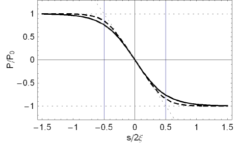
Figure 3: Profile of the ”reversed” polarization component $P_{\rm r}$ (Eqn. 20) for a domain wall with the shape factor $A=1$ (solid) and $A=3$ (dashed). Both profiles have the same derivative for $s/2\xi=0$ (dotted) and therefore also the same thickness (indicated by vertical lines) according to the definition in Eqn. (23).

Solution of the Euler-Lagrange equation (16) is well known.art_zhirnov_1958 ; art_houchmandzadeh_lajzerowic_1991 ; art_hudak ; art_cao_cross_prb_1991 ; art_ishibashi_dvorak_1976 We shall follow the procedure of Ref. art_hlinka_marton_intgrferro, . Integrating Eqn. (16) one can obtain the equation:

$$\frac{g}{2}\left(\frac{\partial p}{\partial s}\right)^{2}=f_{\rm EL}(p)$$ (17)

where (see Ref. art_hlinka_marton_prb_2006, )

$$f_{EL}(p)=a_{1}p(s)^{2}+a_{11}p(s)^{4}+a_{111}p(s)^{6}~{}.$$ (18)

The function $f_{\rm EL}(p)$ is a double-well ”Euler-Lagrange” potential with two minima $\pm p_{\infty}$, where

$$p_{\infty}^{2}=\frac{-a_{11}+\sqrt{a_{11}^{2}-3a_{111}a_{1}}}{3a_{111}}.$$ (19)

The differential Eqn. (16) has the analytical solution

$$p(s)=p_{\infty}\frac{{\sinh}({s}/{\xi^{\prime}})}{\sqrt{A+{\sinh}^{2}({s}/{\xi^{\prime}})}}~{},$$ (20)

where

$$A=\frac{3a_{111}p_{\infty}^{2}+a_{11}}{2a_{111}p_{\infty}^{2}+a_{11}}~{}.$$ (21)

and

$$\xi^{\prime}=\frac{\xi}{\sqrt{A}}~{}.$$ (22)

Quantity $A$ determines deviation of the profile (20) from the $tanh$ profile, which occurs for the $4^{th}$-order potential (i.e., $a_{111}=0,\ A=1$).

The domain wall thickness (Fig. 3) is defined as

$$2\xi=p_{\infty}\sqrt{\frac{2g}{U}}~{}.$$ (23)

with $U$ being the energy barrier between the domain states:

$$U=f_{EL}(0)-f_{EL}(p_{\infty})=2a_{111}p_{\infty}^{6}+a_{11}p_{\infty}^{4}~{}.$$ (24)

The surface energy density of the domain wall is

$$\Sigma = \int_{-\infty}^{\infty}\left(f_{EL}(s)-f_{EL}(p_{\infty})\right)ds$$ (25)

$$= \frac{4}{3}p_{\infty}\sqrt{2gU}\left[A^{5/2}I(A)\right]~{},$$

where

$$I(A)=\frac{3}{4}\int_{-\infty}^{\infty}\frac{{\rm cosh}^{2}(h)dh}{(A+{\rm cosh}^{2}(h)-1)^{3}}~{}.$$ (26)

The domain wall characteristics depend on the coefficients $g,\ a_{1},\ a_{11},\ a_{111}$ through Eqs. (19, 20, 23, 25). The explicit expressions for these coefficients are summarized for various domain walls in Table II. The expressions are simplified using the notation inspired by Ref. art_cao_cross_prb_1991, . For all phases we are using:

$$a_{1}^{\rm r} = \alpha_{1}-\left[\frac{1}{3}\frac{\hat{q}_{11}^{2}}{\hat{C}_{11}}+\frac{1}{6}\frac{\hat{q}_{22}^{2}}{\hat{C}_{22}}-\frac{(q_{11}+q_{12})q_{12}^{\prime}}{2C_{11}^{\prime}}\right]P_{0}^{2}$$

$$a_{11}^{\rm r} = \frac{\alpha_{11}^{(e)}}{2}+\frac{\alpha_{12}^{(e)}}{4}-\frac{q_{12}^{\prime 2}}{2C_{11}^{\prime}}$$

$$a_{12}^{\rm rs} = 3\alpha_{11}^{(e)}-\frac{\alpha_{12}^{(e)}}{2}-\frac{q_{11}^{\prime}q_{12}^{\prime}}{C_{11}^{\prime}}-\frac{\hat{q}_{22}^{2}}{2\hat{C}_{22}}$$

$$a_{111}^{\prime} = \frac{1}{4}\left(\alpha_{111}+\alpha_{112}\right)$$

$$a_{112}^{\prime} = \frac{1}{4}\left(15\alpha_{111}-\alpha_{112}\right)~{},$$

for tetragonal and orthorhombic phases we are abbreviating

$$C_{11}^{\prime} = \frac{C_{11}+C_{12}+2C_{44}}{2}$$

$$C_{12}^{\prime} = \frac{C_{11}+C_{12}-2C_{44}}{2}$$

$$C_{66}^{\prime} = \frac{C_{11}-C_{12}}{2}$$

$$q_{11}^{\prime} = \frac{q_{11}+q_{12}+q_{44}}{2}$$

$$q_{12}^{\prime} = \frac{q_{11}+q_{12}-q_{44}}{2}$$

$$q_{66}^{\prime} = q_{11}-q_{12}~{},$$

and for the rhombohedral phase

$$C_{33}^{\prime} = \frac{C_{11}+C_{12}+2C_{44}}{2}$$

$$q_{11}^{\prime} = \frac{q_{11}+2q_{12}+2q_{44}}{3}$$

$$q_{13}^{\prime} = \frac{q_{11}+2q_{12}-q_{44}}{3}~{}.$$ (27)

The expressions for the coefficients of the T180 and T90 domain walls are equivalent to the previously published expressions.art_cao_cross_prb_1991 ; art_hlinka_marton_prb_2006 Derivations for O60, O120, and R180{$\bar{2}$11} walls lead to complicated formulas, and therefore only numerical results for $g,a_{1},a_{11}$, and $a_{111}$ coefficients are presented here.

Table 2: Parameters characterizing various mechanically compatible and neutral domain wall species of BaTiO₃-like ferroelectrics within the SPP treatment described in the Section IV. Results for O60, O120, and R180{$\bar{2}$11} walls as well as a few other parameters are omitted because the corresponding analytical expressions through the GLD model parameters and spontaneous values of polarization and strain are too complicated.

Domain wall	$p_{\infty}$	$g$	$a_{1}$	$a_{11}$	$a_{111}$
Tetragonal phase
T180{001}	$P_{0}$	$G_{44}$	$\alpha_{1}-e_{\parallel}q_{11}-e_{\perp}q_{12}+\frac{C_{12}}{C_{11}}(e_{\parallel}+e_{\perp})q_{12}$	$\alpha_{11}^{(e)}-\frac{1}{2}\frac{q_{12}^{2}}{C_{11}}$	$\alpha_{111}$
T180{011}	$P_{0}$	$G_{44}$	$\alpha_{1}-e_{\parallel}q_{11}+\frac{C_{12}}{C_{11}^{\prime}}e_{\parallel}q_{12}-2\frac{C_{44}}{C_{11}^{\prime}}e_{\perp}q_{12}$	$\alpha_{11}^{(e)}-\frac{1}{2}\frac{q_{12}^{2}}{C_{11}^{\prime}}$	$\alpha_{111}$
T90	$\frac{P_{0}}{\sqrt{2}}$	$\frac{G_{11}-G_{12}}{2}$	$\alpha_{1}^{\rm r}+\alpha_{12}^{\rm rs}\frac{P_{0}^{2}}{2}+\alpha_{112}^{\prime}\frac{P_{0}^{4}}{4}$	$\alpha_{11}^{\rm r}+\alpha_{112}^{\prime}\frac{P_{0}^{2}}{2}$	$\alpha_{111}^{\prime}$
Orthorhombic phase
O180{1$\bar{1}$0}	$P_{0}$	$\frac{G_{11}-G_{12}}{2}$	$\alpha_{1}-e_{\rm b}(q_{11}^{\prime}-q_{12}^{\prime})-e_{\rm c}q_{12}-e_{\rm a}(q_{11}^{\prime}+q_{12}^{\prime})$	$\frac{\alpha_{11}^{(e)}}{2}+\frac{\alpha_{12}^{(e)}}{4}-\frac{q_{12}^{\prime 2}}{2C_{11}^{\prime}}$	$\frac{1}{4}\left(\alpha_{111}+\alpha_{112}\right)$
			$+\frac{q_{12}^{\prime 2}}{C_{11}^{\prime}}P_{0}^{2}$
O180{001}	$P_{0}$	$G_{44}$	$\alpha_{1}-e_{\rm a}(q_{11}+q_{12})-e_{\rm b}q_{44}+2e_{\rm a}q_{12}\frac{C_{12}}{C_{11}}$	$\frac{\alpha_{11}^{(e)}}{2}+\frac{\alpha_{12}^{(e)}}{4}-\frac{q_{12}^{2}}{2C_{11}}$	$\frac{1}{4}\left(\alpha_{111}+\alpha_{112}\right)$
O90	$\frac{P_{0}}{\sqrt{2}}$	$G_{44}$	$\alpha_{1}^{\rm r}+\alpha_{12}^{\rm(e)}\frac{P_{0}^{2}}{2}+\alpha_{112}\frac{P_{0}^{4}}{4}$	$\alpha_{11}^{(e)}+\frac{1}{2}\left[\alpha_{112}P_{0}^{2}-\frac{q_{12}^{2}}{C_{11}}\right]$	$\alpha_{111}$
O120	$\frac{\sqrt{3}P_{0}}{2}$	$\frac{G_{11}-G_{12}+4G_{44}}{6}$	***	***	$\frac{2\alpha_{111}+21\alpha_{112}+2\alpha_{123}}{108}$
Rhombohedral phase
R180{1$\bar{1}$0}	$P_{0}$	$\frac{G_{11}-G_{12}+G_{44}}{3}$	$\alpha_{1}+\frac{1}{6C_{33}^{\prime}}[C_{12}(e_{\rm a}(q_{11}+2q_{12}-4q_{44})-6e_{\rm b}q_{44})$	$\frac{\alpha_{11}^{(e)}+\alpha_{12}^{(e)}}{3}-\frac{q_{13}^{\prime 2}}{2C_{33}^{\prime}}$	$\frac{3\alpha_{111}+6\alpha_{112}+\alpha_{123}}{27}$
			$-C_{11}(6e_{\rm b}q_{44}+3e_{\rm a}q_{11}^{\prime})$
			$-2C_{44}(3e_{\rm a}(q_{11}+2q_{12})+6e_{\rm b}q_{11}^{\prime})]$
R180{$\bar{2}$11}	$P_{0}$	$\frac{G_{11}-G_{12}+G_{44}}{3}$	***	***	$\frac{3\alpha_{111}+6\alpha_{112}+\alpha_{123}}{27}$
R109	$\frac{P_{0}}{\sqrt{3}}$	$G_{44}$	$\alpha_{1}+\frac{\alpha_{12}^{(e)}P_{0}^{2}}{3}+\frac{\alpha_{112}P_{0}^{4}}{9}+\frac{2q_{12}^{2}P_{0}^{2}}{3C_{11}}-\frac{q_{44}^{2}P_{0}^{2}}{6C_{44}}$	$\frac{\alpha_{11}^{(e)}}{2}+\frac{\alpha_{12}^{(e)}}{4}-\frac{q_{12}^{2}}{2C_{11}}$	$\frac{\alpha_{111}+\alpha_{112}}{4}$
			$-e_{\rm a}(q_{11}+2q_{12})-e_{\rm b}q_{44}$	$+\frac{1}{12}\left(2\alpha_{112}+\alpha_{123}\right)P_{0}^{2}$
R71	$\frac{P_{0}}{\sqrt{3}}$	$G_{44}$	$\alpha_{1}+\frac{2\alpha_{12}^{(e)}P_{0}^{2}}{3}+\frac{2\alpha_{112}P_{0}^{4}}{9}+\frac{\alpha_{123}P_{0}^{4}}{9}$	$\alpha_{11}^{(e)}+\frac{2\alpha_{112}P_{0}^{2}}{3}-\frac{q_{12}^{2}}{2C_{33}^{\prime}}$	$\alpha_{111}$
			$-e_{\rm a}(q_{11}+2q_{12})+\frac{q_{12}^{2}P_{0}^{2}}{3C_{33}^{\prime}}-\frac{q_{44}^{2}P_{0}^{2}}{3C_{44}}$

V QUANTITATIVE RESULTS

Table 3: Predicted values of thickness and planar energy density of domain wall species illustrated in Fig. 2 together with the determining parameters appearing in the SPP treatment. Results are evaluated from the BaTiO₃-specific GLD model at three selected temperatures corresponding to the tetragonal, orthorhombic and rhombohedral phase, respectively. Domain walls for which relaxing of the $P_{\rm t}$ component results in a lower-energy CPP solution (see in Section VI.) are denoted by ^†. Numerical values are in SI units ($2\xi$ in nm; $\Sigma$ in mJ/m²; $U$ in MJ/m³; $p_{\infty}$ in C/m²; $g$ in 10^-11 kg m⁵ s^-2 C^-2; $a_{1}$ in 10⁷ kg m³ s^-2 C^-2; $a_{11}$ in 10⁸ kg m⁷ s^-2 C^-4; $a_{111}$ in 10⁹ kg m¹¹ s^-2 C^-6).

Domain wall	$2\xi$	$\Sigma$	$U$	$A$	$~{}~{}~{}~{}~{}~{}~{}~{}~{}~{}p_{\infty}$	$g$	$a_{1}$	$a_{11}$	$a_{111}$
Tetragonal phase (298 K)
T180{001}	0.63	5.9	6.41	1.43	0.265	2.0	-14.26	1.69	8.00
T180{011}	0.63	5.9	6.41	1.43	0.265	2.0	-14.26	1.69	8.00
T90	3.59	7.0	1.45	1.09	0.188	26.5	-7.86	9.53	3.12
Orthorhombic phase (208 K)
O180{1$\bar{1}$0}†	2.66	31.0	8.20	1.70	0.331	26.5	-9.71	-2.75	4.36
O180{001}	0.70	8.9	8.95	1.64	0.331	2.0	-11.07	-2.13	4.36
O90	0.72	4.3	4.26	1.50	0.234	2.0	-11.62	-0.08	12.97
O60	3.62	5.3	1.09	1.08	0.166	26.1	-7.64	12.14	4.36
O120†	1.70	13.7	5.82	1.47	0.287	10.2	-10.82	0.50	4.92
Rhombohedral phase (118 K)
R180{1$\bar{1}$0}†	2.13	36.0	11.81	1.83	0.381	18.3	-9.53	-3.64	3.17
R180{$\bar{2}$11}†	2.13	36.0	11.81	1.83	0.381	18.3	-9.53	-3.64	3.17
R109†	0.70	7.8	7.81	1.65	0.311	2.0	-10.84	-2.56	5.60
R71	0.74	3.7	3.52	1.58	0.220	2.0	-10.31	-2.42	17.94

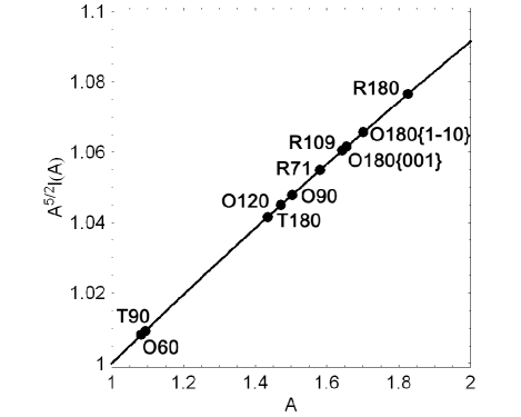
Figure 4: Dependence of correction factor in the expression for domain wall energy density (25) as a function of the shape coefficient $A$. Full points indicate values of $A$ for particular domain walls considered in Table III.

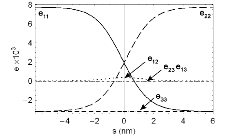
Figure 5: Course of strain components along the domain wall normal coordinate $s$ for the T90 domain wall. Indices refer to cubic axes of the parent phase.

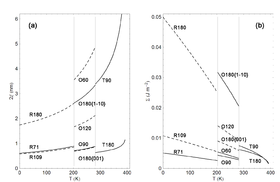
Figure 6: Temperature dependence of the thickness (a) and energy density (b) for various mechanically compatible and neutral domain walls of BaTiO₃ estimated within SPP approximation. The SPP values for domain walls for which relaxing of the $P_{\rm t}$ component results in a lower-energy CPP solution (see in Section VI.) are shown by dashed lines. Thickness of O180{001}, O90 has a very close temperature dependence. The results for T180 as well as for R180 walls are not distinguished by specific orientations of the wall normal, since for both cases the angular dependence of thickness and energy of SPP solutions on the domain wall normal is negligible (see Tab. 3). Vertical lines mark phase-transition temperatures.

Advantage of the GLD approach is that domain wall properties can be obtained at any temperature. In Table 3 we give numerical results for domain wall parameters at one particular temperature for each of the ferroelectric phases: at 298 K, 208 K, and 118 K for the tetragonal, orthorhombic, and rhombohedral phase, resp. Corresponding numerical values of the spontaneous quantities appearing in Table 1 are: $P_{0}=0.265\,{\rm C\,m^{-2}}$, $e_{\parallel}=Q_{11}P_{0}^{2}=7.77\times 10^{-3}$ and $e_{\perp}=Q_{12}P_{0}^{2}=-3.18\times 10^{-3}$ (the tetragonal phase, 298 K); $P_{0}=0.331\,{\rm C\,m^{-2}}$, $e_{\rm a}=\frac{Q_{11}+Q_{12}}{2}P_{0}^{2}=3.58\times 10^{-3}$, $e_{\rm c}=Q_{12}P_{0}^{2}=-4.96\times 10^{-3}$ and $e_{\rm b}=\frac{Q_{44}}{4}P_{0}^{2}=0.79\times 10^{-3}$ (the orthorhombic phase, 208 K); $P_{0}=0.381\,{\rm C\,m^{-2}}$, $e_{\rm a}=\frac{Q_{11}+2Q_{12}}{3}P_{0}^{2}=0.97\times 10^{-3}$ and $e_{\rm b}=\frac{Q_{44}}{4}P_{0}^{2}=0.70\times 10^{-3}$ (the rhombohedral phase, 118 K). The base vectors for the O60 domain wall (see Eqn. 3) at 208 K are

$${\bf r}_{\rm O60} = \left(0.707,0,0.707\right)$$

$${\bf s}_{\rm O60} = \left(0.701,0.130,-0.701\right)$$

$${\bf t}_{\rm O60} = \left(-0.092,0.991,0.092\right)~{}.$$ (28)

The right four columns of the Table 3 contain corresponding numerical values of the domain wall coefficients $g$, $a_{1}$, $a_{11}$, and $a_{111}$ derived from GLD parameters and spontaneous order-parameter values using above derived analytical expressions, mostly given explicitly in Table 2. The left part of the Table 3 contains the key domain wall properties such as wall thickness $2\xi$ and energy density $\Sigma$.

Clearly, T90 and O60 domain walls are considerably broader then others. T90 wall in the tetragonal phase is predicted to be 3.59 nm thick at 298 K (as already calculated in Ref. art_hlinka_marton_prb_2006, ) and S-type O60 domain wall in the orthorhombic phase is predicted to be 3.62 nm thick at 208 K. Since the wall thickness is greater than the lattice spacing, the pinning of the walls is weakart_ishibashi and they can be easily moved. Moreover, in case of O60 wall, the pinning is further suppressed due to ’incommensurate’ character of Miller indices of the wall normal.

As follows from Eqn. (23), domain wall thickness is determined by quantities $g$, $U$, and $p_{\infty}$. By inspection of their values in Table 3, we see that the most important factor is the coefficient $g$. Indeed, the domain walls R71, R109, O90, O180{001}, T180 with $g=2\times 10^{-11}~{}{\rm kg\,m^{5}s^{-2}\,C^{-2}}$ are all very narrow (thickness below $1$ nm), and the thickness of various walls monotonically increases with increasing value of $g$. Let us stress that coefficients $a_{1}$, $a_{11}$, $a_{111}$, and $g$ depend on the direction of the domain wall normal. For example, O180{1$\bar{1}$0} with $g=26.5\times 10^{-11}~{}{\rm kg\,m^{5}s^{-2}\,C^{-2}}$ is almost four times broader than O180{001} with $g=2\times 10^{-11}~{}{\rm kg\,m^{5}s^{-2}\,C^{-2}}$.

In the absence of other constraints, the probability of appearance of domain wall species should be determined by the surface energy density $\Sigma$. Therefore, in the orthorhombic phase, the thinner O180$\{001\}$ wall is more likely to occur than the 0180$\{1\bar{1}0\}$ one. Interestingly, the O180$\{001\}$ wall has almost the same thickness as the O90 wall, while in the tetragonal phase, it is the 90^∘ wall which is much thicker than 180^∘ wall (3.59 nm compared to 0.63 nm).

In general, the normal of the neutral 180^∘-domain wall can take any direction perpendicular to the spontaneous polarization of the adjacent domains. Therefore also $\Sigma$ depends on the orientation of the wall normal (in the $s-t$ plane). We have checked in the orthorhombic phase that the 0180$\{001\}$ and 0180$\{1\bar{1}0\}$ correspond to the extremes in the angular dependence of $\Sigma$, which is monotonous between them. This strong angular dependence is correlated with the anisotropy of the tensor $G_{ijkl}$. However, $g$ is independent of the wall direction in the tetragonal and rhombohedral phase, and also the variation of coefficients $a_{1}$, $a_{11}$, and $a_{111}$ is insignificantly small, so that the effective directional dependence of 180^∘ domain wall properties in these phases is negligible.

The values of the shape factor $A$ (see Table 3) determines the deviation of the $P_{\rm r}(s)$ polarization profile of the domain walls from the simple $tanh$ form. For all studied cases the values of $A$ range between 1 and 2, where the correction factor $A^{5/2}I(A)$ appearing in the Eqn. (25) is almost linear function of $A$, as it can be seen in Fig. 4. It means that the shape deviations are much smaller than those shown by broken line in Fig. 3. Unfortunately, in the case of broad walls T90 and O60, which are good candidates for study of the structure of the wall central part, $A$ is almost one.

Eqn. (14) can be also used to evaluate local strain variation in the wall. In Fig. 5 the profiles of strain tensor components for T90 domain wall are shown for illustration. Obviously, $e_{33},e_{23}$, and $e_{13}$ strain components are strictly constant and equal to their boundary values as it follows from mechanical compatibility conditions. The $e_{11}$ and $e_{22}$ components and polarization $P_{\rm r}$ vary between their spontaneous values. Let us stress that the ’re-entrant’ shear component $e_{12}$ (it has the same value in both adjacent domains) approaches the non-zero value of about 5$\times 10^{-4}$ in the middle of the domain wall.

The temperature dependence of the thickness and surface energy density of the 12 studied domain wall species is plotted in Fig. 6a and Fig. 6b, respectively. Although some properties do vary considerably, e.g. thickness of T90 wall in the vicinity of the paraelectric-ferroelectric phase transition, the sequence of the thickness values as well as the surface energy-density values of different domain wall types remain conserved within each phase.

The temperature dependence of domain wall thickness follows the trend given by Eqn. (23). It increases with increasing temperature due to the dependence on $p_{\infty}$ (see dependence of $U$ on $p_{\infty}$ in Eqn. (24)). Such behavior is well known also from the experimental observations.art_andrews_1986 ; art_robert_1996 ; art_huang_jiang_hu_liu_JPCM_1996

VI CURVED POLARIZATION PATH SOLUTIONS

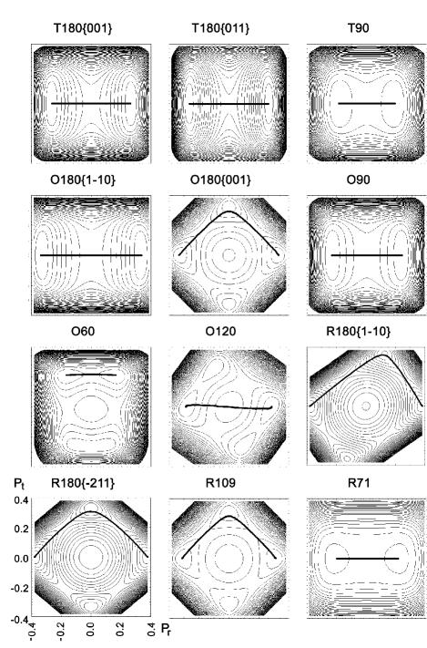
Figure 7: Equipotential contours of the Euler-Lagrange potentials showing ELPS associated with the $P_{\rm s}$=$P_{\rm s}(\pm\infty)$ plane for a set of BaTiO₃ domain walls considered in Table III. Polarization scale given for the bottom left inset (in Cm^-2) is equally valid for all shown ELPS’s. Energetically most favorable domain wall solutions with trajectories restricted to the $P_{\rm s}$=$P_{\rm s}(\pm\infty)$ plane are indicated with bold lines. The solutions corresponding to a linear segment are denoted in the text as SPP walls, as opposed to the CPP solutions (see in Section VI.), which have a curved order-parameter trajectory.

So far we have investigated domain walls within the SPP approximation, i.e. components $P_{\rm s}$ and $P_{\rm t}$, which are the same in both domain states, were kept constant inside the whole wall. This is quite usual assumption made for a ferroelectric domain wall. Nevertheless, the full variational problem, where all three components of $\bf P$ could vary along $\bf s$ coordinate, leads in general to a lower energy solution corresponding to a curved polarization path (CPP) in the 3D primary order-parameter space. Appearance of the non-zero ’re-entrant’ components within a ferroelectric domain wall was considered e.g. in works of Refs. art_huang_jiang_hu_liu_JPCM_1996, ; art_hlinka_marton_prb_2006, ; art_lee_2009, ; art_meyer_vanderbilt_2002, . For 180^∘ walls, the polarization profile associated with SPP is sometimes denoted as the Ising-type wall. In contrast, the CPP solutions with non-zero $P_{\rm s}$, $P_{\rm t}$ are often considered as Néel and Bloch-like,art_lee_2009 even though, in contrast with magnetism, the modulus of $\bf P$ is far from being conserved along the wall normal $\bf s$.

We have previously considered non-constant $P_{\rm s}$ component of polarization in the 90^∘ wall with explicit treatment of electrostatic interaction and realized that the deviations from SPP approximation are quite negligible.art_hlinka_marton_prb_2006 In general, non-constant $P_{\rm s}$ would lead to non-vanishing $\nabla\cdot\bf{\rm P}$ and finite local charge density, which in a perfect dielectric causes a severe energy penalty. The same situation is expected for all domain wall species. However, there is no such penalty for non-constant $P_{\rm t}$-solutions. It was previously arguedart_huang_jiang_hu_liu_JPCM_1996 that the Bloch-like (with a considerable magnitude of $P_{\rm t}$ at the domain wall center) solutions could occur in orthorhombic BaTiO₃. Therefore, it is interesting to systematically check for existence of such solutions using our model.

In order to study such Bloch-like solutions, we have calculated Euler-Lagrange potential in the order-parameter plane $P_{\rm s}=P_{\rm s}(\pm\infty)$ by integrating Euler-Lagrange equations (Eqn. 13 and 14) for all domain wall species from Table 3 similarly as e.g. in the Refs. art_cao_cross_prb_1991, ; art_huang_jiang_hu_liu_JPCM_1996, . Resulting 2D Euler-Lagrange potential surfaces (ELPS) are displayed in Fig. 7. In each ELPS, the bold lines indicate numerically obtained domain-wall solution with the lowest energy. The spatial step was chosen as 0.1 nm, $P_{\rm r}$ and $P_{\rm t}$ were fixed to boundary conditions in sufficient distance from domain wall (6 nm) and initial conditions for $P_{\rm t}$ were chosen so that the polarization path bypasses the energy maximum of the ELPS, and the system was relaxed to the equilibrium.

Among the twelve treated wall species, there are six cases where only the SPP solutions with $P_{\rm t}$=const exist: T180{001}, T180{011}, T90, O180{1$\bar{1}$0}, O90, and R71. These solutions are clearly ”Ising-like”. In all these cases, the ($P_{\rm r}=0$, $P_{\rm t}=0$) point is the only saddle point of the ELPS. In the other six cases – O180{001}, O60, O120, R180{1$\bar{1}$0}, R180{$\bar{2}$11}, and R109 – the ELPS has a maximum at the ($P_{\rm r}=0$, $P_{\rm t}=0$), and the lowest energy solutions correspond to curved polarization paths. This suggests that the previously discussed SPP description may not necessarily be the proper approximation for these walls. Nevertheless, in the case of O60 and O120 walls the deviations from the SPP model are marginal, and only the remaining four solutions exhibit strong Bloch-like behavior. Moreover, the energy differences between SPP and CPP solutions were found to be almost negligible, except for R180, where the CPP energy is by about 10% lower in the entire temperature range of stability of the rhombohedral phase. Therefore, it is quite possible that in the case of O180{001}, R180{1$\bar{1}$0}, R180{$\bar{2}$11}, and R109 walls both Bloch-like and Ising-like solutions may be realized.

The deviations from SPP in the case of the almost Ising-like O60 and O120 walls are associated with the fact that ELPS is not symmetric with respect to $P_{\rm t}=P_{\rm t}(\pm\infty)$ mirror plane. In these cases not only the polarization path and wall energies, but also domain wall thicknesses of the SPP and CPP counterpart solutions are very similar. This is demonstrated in Fig. 8, which shows polarization profiles of both SPP and CPP solutions for the O60 wall.

Much more pronounced difference between domain wall profiles of SPP and CPP solutions are found in case of O180{001}, R180{1$\bar{1}$0}, R180{$\bar{2}$11}, and R109 Bloch-like walls where the CPP trajectories bypass the ($P_{\rm r}=0$, $P_{\rm t}=0$) maximum near the additional minima, which originate from ’intermediate’ domain states either of the same phase or even of the different ferroelectric phases. In these cases, the inadequacy of SPP approximation is obvious. For example, the CPP of R180{$\bar{2}$11} wall seems to pass through a additional minimum corresponding to an ’orthorhombic’ polarization state (consult corresponding inset in the Fig. 2). As expected, the profile of such CPP solution deviates strongly from $tanh$ shape and even definition of the wall thickness would be problematic (see Fig. 9).

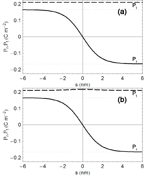
Figure 8: Predicted profiles of polarization components for O60 domain wall in BaTiO₃ at $T=208\,$K. Full line stands for the $P_{\rm r}$ component of polarization vector, broken line for the $P_{\rm t}$ one. Analytically obtained SPP solution (a) practically does not differ from the numerically obtained CPP solution (b) with an unconstrained $P_{\rm t}$ component in this case.

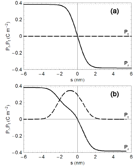
Figure 9: Profiles of polarization components in R180{1$\bar{1}$0} domain wall showing the SPP stationary trajectory (a) as well as the lower energy Bloch-like solution (b), both for the model parameters corresponding to $T=118\,$K. Full line stands for the $P_{\rm r}$ component of polarization vector, broken line for the $P_{\rm t}$ one. The bottom panel demonstrates that Bloch solution may considerable modify the domain domain wall profile.

VII CONCLUSION

The work reports detailed study of mechanically compatible and electrically neutral domain walls in BaTiO₃. The investigation was done within the framework of the GLD model. Using the SPP approximation it was possible to compare properties of various kinds of domain wall species from the same perspective.

The phenomenological nature of the GLD model allowed to predict the temperature dependence of the domain wall characteristics in the whole temperature range of ferroelectric phases. Its continuous nature gave us even the opportunity to deal conveniently with the non-crystallographic S-type domain wall, which has a general orientation with respect to the crystal lattice, and which is therefore difficult to cope with in discrete models relying on periodic boundary conditions.

The S-wall in the orthorhombic, as well as the 90^∘ wall in tetragonal phase were both found to be about 4 nm thick and consequently are expected to be mobile, i.e. they could be easily driven by external fields, and they may thus significantly contribute to the dielectric or piezoelectric response of the material.

For several temperatures, we have numerically investigated domain walls allowing for more complicated CPP solutions with non-constant $P_{\rm t}$. We have identified solutions, which could be considered as analogues of Bloch walls known from magnetism. Interestingly, in contrast with Ref. art_huang_jiang_hu_liu_JPCM_1996, , our model predicts the Ising-type profile of the O180{1$\bar{1}$0} wall. At the same time the Bloch-like structure of the O180{001} wall is predicted.

We believe that this kind of somewhat exotic walls actually represent important generic examples of ferroelectric domain species, which should be anticipated in all ferroelectrics with several equivalent domain states distinguished simultaneously by the orientation of the spontaneous polarization and strain. They should be certainly taken into account in investigations of domain-wall phenomena in ferroelectric perovskites. At the same time, the energy differences between the Bloch-like and Ising-like solutions are rather subtle here. Therefore, in spite of the fairly good agreement for 180^∘ and 90^∘ domain walls between ab-initio calculations and predictions of this model in the tetragonal phase,art_hlinka_marton_prb_2006 the preference for the calculated Bloch-like trajectories may not necessarily reproduced for the domain walls encountered in real BaTiO₃ crystal, since there is obviously a considerable uncertainty in the adopted material-specific GLD parameters. In addition, predictions for the domain walls with very small thickness must be considered with a particular caution since the description of the sharp domain wall profiles obviously touches the limits of the applicability of the continuous model.

In conclusion, we have derived a number of qualitative and quantitative predictions for mechanically compatible neutral domain walls of tetragonal, orthorhombic and rhombohedral BaTiO₃ on the basis of the previously proposed material-specific GLD model. We believe that the insight into the domain wall properties mediated by the provided analytical and numerical analysis could be helpful for understanding of domain wall phenomena in BaTiO₃ as well as in some other intensively investigated members of the ferroelectric perovskite family with same sort of macroscopic ferroelectric phases, for example in KNbO₃, BiFeO₃, PbTiO₃ or even PZT and perovskite relaxor-related materials.

References

• (1) W. Cao and L. E. Cross, Phys. Rev. B 44, 5 (1991).
• (2) Y. Ishibashi and E. Salje, J. Phys. Soc. Jpn. 71, 2800 (2002).
• (3) X. R. Huang, S. S. Jiang, X. B. Hu, and W. J. Liu, J. Phys.: Condens. Matter 9, 4467 (1997).
• (4) J. Hlinka and P. Marton, Phys. Rev. B 74, 104104 (2006).
• (5) J. Erhart, W. Cao, and J. Fousek, Ferroelectrics 252, 137 (2001).
• (6) S. Nambu and D. A. Sagala, Phys. Rev. B 50, 5838 (1994).
• (7) H. L. Hu and L. Q. Chen, J. Am. Ceram. Soc. 81, 492 (1998).
• (8) R. Ahluwalia, T. Lookman, A. Saxena, and W. Cao, cond-mat/0308232 (2003).
• (9) P. Marton and J. Hlinka, Phase Transitions 79, 467 (2006).
• (10) J. Fousek and V. Janovec, J. Appl. Phys. 40, 135 (1969).
• (11) V. Janovec and J. Privratska, Domain structures, in International Tables for Crystallography (Kluwer Academic Publishers, Dordrecht, 2003), Ch. 3.4., vol. D.
• (12) J. Fousek, Czech J. Phys. B 21, 955 (1971).
• (13) A. J. Bell, J. Appl. Phys. 89, 3907 (2001).
• (14) In the final phase of preparation of this paper it turned out that the value of $q_{44}$ should be multiplied by a factor of two.art_hlinka_ondrejkovic_nano_2009 Considering the general character of this paper, we have left the original value of $q_{44}$, which is being used in some previous works reffered to here. The changes in results are minor ones and they can be traced using provided analytical expressions.
• (15) J. Hlinka, P. Ondrejkovic, and P. Marton, Nanotechnology 20, 105709 (2009).
• (16) V. A. Zhirnov, Zh. Eksp. Teor. Fiz. 35, 1175 (1959), [Sov. Phys. JETP 8, 822 (1959)].
• (17) O. Hudak , arXiv:cond-mat/0504701 (2005).
• (18) Y. Ishibashi and V. Dvorak, J. Phys. Soc. Jpn. 41, 1650 (1976).
• (19) B. Houchmandzadeh, J. Lajzerowic, and E. Salje, J. Phys.: Condens. Matter 3, 5163 (1991).
• (20) J. Hlinka and P. Marton, Integrated Ferroelectrics 101, 50 (2008).
• (21) Y. Ishibashi, J. Phys. Soc. Jpn. 46, 1254 (1979).
• (22) M. Robert, I. Reaney, and P. Stadelmann, Physica A 229, 47 (1996).
• (23) S. R. Andrews and R. A. Cowley, J. Phys. C: Solid State Phys. 19, 615 (1986).
• (24) B. Meyer and D. Vanderbilt, Phys. Rev. B 65, 104111 (2002).
• (25) D. Lee, R. K. Behera, P. Wu, H. Xu, S. B. Sinnott, S. R. Phillpot, L. Q. Chen, and V. Gopalan, Phys. Rev. B 80, 060102(R) (2009).