Extinction in Star-Forming Disk Galaxies from Inclination-Dependent Composite Spectra

Abstract

Extinction in galaxies affects their observed properties. In scenarios describing the distribution of dust and stars in individual disk galaxies, the amplitude of the extinction can be modulated by the inclination of the galaxies. In this work we investigate the inclination dependency in composite spectra of star-forming disk galaxies from the Sloan Digital Sky Survey Data Release 5. In a volume-limited sample within a redshift range $0.065-0.075$ and a $r$-band Petrosian absolute magnitude range -19.5 to -22 mag which exhibits a flat distribution of inclination, the inclined relative to face-on extinction in the stellar continuum is found empirically to increase with inclination in the $g$, $r$ and $i$ bands. Within the central $0.5$ intrinsic half-light radius of the galaxies, the $g$-band relative extinction in the stellar continuum for the highly-inclined objects (axis ratio $b/a=$ 0.1) is 1.2 mag, agreeing with previous studies. The extinction curve of the disk galaxies is given in the restframe wavelengths $3700-8000$ Å, identified with major optical emission and absorption lines in diagnostics. The Balmer decrement, H$\alpha$/H$\beta$, remains constant with inclination, suggesting a different kind of dust configuration and/or reddening mechanism in the H II region from that in the stellar continuum. One factor is shown to be the presence of spatially non-uniform interstellar extinction, presumably caused by clumped dust in the vicinity of the H II region.

1 Introduction

Extinction in galaxies affects their observed properties. Ideally it should be taken into account when inferring the intrinsic properties of the galaxies. One empirical approach in studying extinction in disk galaxies is to compare the observed properties of objects with similar intrinsic properties at different inclination (Holmberg, 1958). Optically thin galaxies, when inclined, should show higher surface-brightness than their face-on counterparts because of a larger column of stars observed in a smaller projected area on the sky. This approach has been adopted into various analyses by many authors to study extinction in disk galaxies (e.g., Disney et al., 1989; Valentijn, 1990; Huizinga & van Albada, 1992; Davies et al., 1993; Giovanelli et al., 1994; Boselli & Gavazzi, 1994; Davies & Burstein, 1995).

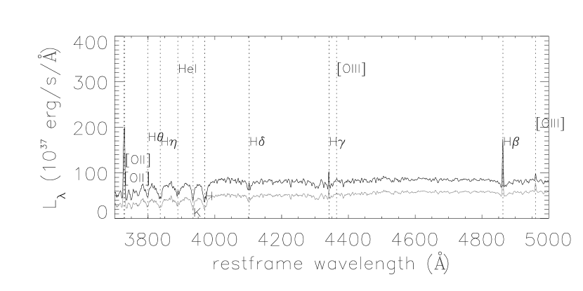
Figure 6: The comparison between the restframe composite spectra of face-on ($b/a=0.9-1.0$, black) and edge-on ($b/a=0.1-0.2$, gray) star-forming disk galaxies, for the volume-limited sub-sample. The flux density per unit wavelength is an “observed” quantity in the sense that inclination correction is not applied.

Recently, there are revived interests on the topic of extinction because of the large sample of galaxies made available by various sky surveys including the Sloan Digital Sky Survey (SDSS; York et al., 2000). Progress has been made in studying extinction in galaxies empirically by using techniques that are depend on or independent of the inclination-related approach. Shao et al. (2007) demonstrated the inclination dependency of dust extinction in disk-dominated galaxies from the SDSS, by using the $z$-band extinction, and an inclination measure being the apparent major to minor axes ratio. Holwerda et al. (2007) applied the technique of occulting galaxy pairs (White & Keel, 1992) to 83 SDSS spiral disk galaxies in in probing the opacity of the foreground galaxies, and found that the optical depths ($\tau$) in the $g$, $r$, $i$ bands are typically within the range $0-1.5$ across the disk from approximately ${0.5}$ to ${4}$ half-light radii ($r_{\rm eff}$, in their Figure 6). Unterborn & Ryden (2008) looked at disk-dominated galaxies from the SDSS and found that the highly inclined objects ($b/a\sim{0.1}$) exhibit $\sim{1}$ mag extinction correction relative to the face-on magnitude. Maller et al. (2009) studied the observed photometric properties of the SDSS galaxies as a function of inclination, and concluded that the inclination-dependent extinction correction in the $g$ band could reach $\sim{1}$ mag with a median value of 0.3 mag for a sample of disk galaxies. Bailin & Harris (2008) applied the inclination-corrected magnitudes to the context of galaxy classification. Driver et al. (2007) developed a sophisticated approach to derive iteratively the extinction-inclination relation for both the bulge and disk components of disk galaxies, and found that the edge-on to face-on relative extinction is $\approx~{}{2}$ mag and $\approx~{}{1}$ mag, respectively for the bulge and the disk. This is an unique approach to date to simultaneously perform the bulge-to-disk decomposition and derive the extinction-inclination relation for both components.

Inspired by these studies, and that the SDSS provides for us a large sample of galaxy spectra within a fixed central 3″-diameter fiber, and that the calibration of the spectra is independent of that in the SDSS photometric data used by Shao et al. (2007), Holwerda et al. (2007), Unterborn & Ryden (2008) and Maller et al. (2009), we now investigate if there is any inclination dependency in the observed galaxy spectra; and what is its wavelength dependency, e.g., the effect in the gaseous component, such as the H II region, vs. that in the stellar continuum; and the comparison of extinctions among different elements. Our approach is to explore the inclination dependency of composite spectra of star-forming disk galaxies in a well defined volume-limited sample that exhibits a flat distribution of the galaxy inclination. The volume-limited nature of the sample eliminates the Malmquist bias in the analysis. The sample is also selected to exhibit a flat distribution of the inclination angle, so that at a chosen redshift ($z$) range, a galaxy of luminosity in a defined range would be observed by the survey, independent of the inclination angle (or other properties) of the galaxy. It is a very important step because one can then assume randomness in the intrinsic properties of the sampled galaxies. We further confine ourselves to a sample of a narrow redshift range, so that any difference detected in the observed properties between the two composite spectra at different inclination would not be mainly due to the difference in the redshifts of the galaxies. On the other hand, the composite spectra, or the sample-average spectra, are used in an effort to average the variation in the intrinsic properties of the galaxies, as the actual optical depth of individual galaxies depends on detailed properties such as the distribution of dust, gas, and stars, the structure of the galaxies such as the presence of arms (e.g. Elmegreen, 1980; Beckman et al., 1996), the Hubble type, etc..

We introduce the galaxy sample in §2. We present results on the inclination dependency of composite spectra of the galaxies in §3. We derive the empirical continuum extinction in the SDSS $g$, $r$, $i$  bands in §4, the model-based face-on extinction in §4.3, and the extinction curve (the extinction as a function of restframe wavelength) in §4.4. We study the relation between the Balmer decrement and the inclination-dependent continuum extinction in §5. We summarize the results in §6.

We use the term “reddening” to refer to the reduction in flux in the shorter wavelengths relative to longer wavelengths, or a decrease in the steepness of the spectral slope. We follow Davies & Burstein (1995) and use the terminology “extinction” to refer to the reduction of flux due to absorption and/or scattering by dust. We use “attenuation” interchangeably with extinction. Following the convention in the SDSS we express the spectra in vacuum wavelengths.

2 The Sample

As part of the Sloan Digital Sky Survey (York et al., 2000) spectra are taken with fibers of 3″  diameter (corresponding to 0.18 mm at the focal plane for the 2.5 m, f/5 telescope). All sources are selected from an initial imaging survey using the SDSS camera described in Gunn et al. (1998) with the filter response curves as described in Fukugita et al. (1996), and using the imaging processing pipeline of Lupton et al. (2001). The astrometric calibration is described in Pier et al. (2003). The photometric system and calibration are described in (Smith et al., 2002; Hogg et al., 2001; Ivezić et al., 2004). The selection criteria of the “Main” galaxies for spectroscopic follow-up observations are discussed by Strauss et al. (2002).

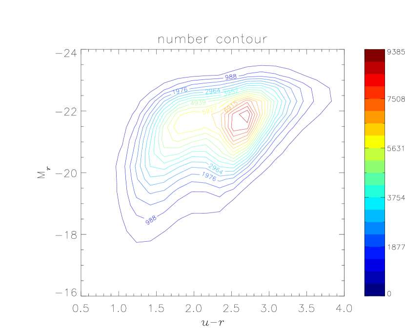
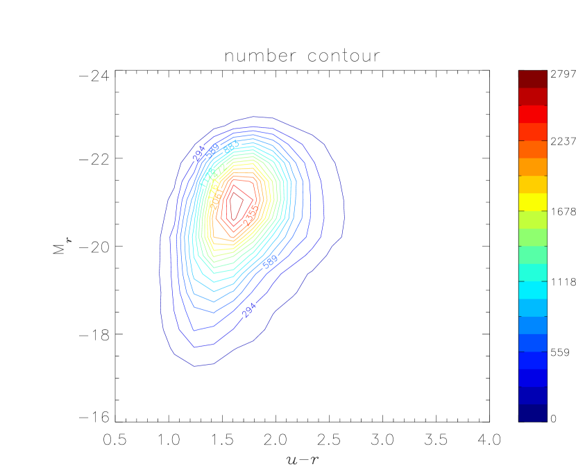
Figure 1: Left: the restframe $r$-band Petrosian absolute magnitude vs. the restframe $u$ - $r$ color for the galaxies in the parent sample. The range of fracDeV_r  is from $0-1$. Both the magnitude and the color are K-corrected. Right: same as the left, but plotted with only the galaxies that lie in a fracDeV_r  range of $0-0.1$. Compared with the left figure, now the blue galaxies are sampled predominantly, with a contamination by the red sequence of $\approx~{}5$%.

Our sample is taken from the spectra of star-forming disk galaxies in the SDSS Data Release 5 (DR5). We determine the criterion for selecting disk-dominated galaxies with the approach used in Unterborn & Ryden (2008), who characterized that galaxies with exponential radial light profiles fall on the blue sequence in the color-magnitude diagram. Based on the full DR5 spectroscopic sample, we define a parent sample of galaxies at redshifts $0-0.2$, which covers the median redshift of the Main galaxy sample, about 0.1 (Strauss et al., 2002). The galaxies in the parent sample have fracDeV_r = $0-1$ in the $r$ band, where fracDeV_r equals $0$ for a pure exponential, and equals $1$ for a pure de Vaucouleurs light profile as provided by the SDSS imaging pipeline (Lupton et al., 2001). The color-magnitude diagram of the parent sample is shown in the left of Figure 1, in the $r$-band Petrosian absolute magnitude, $M_{r}$, vs. $u$ - $r$. Both the absolute magnitudes and the colors are K-corrected, and corrected against foreground dust using the Milky Way dust map (Schlegel et al., 1998). Two main distributions are discernible in the color-magnitude space, corresponding respectively to the red sequence ($u$ - $r$ $>2.4$) and the blue sequence. Based on the parent sample, we determine the appropriate fracDeV_r cut for selecting the blue galaxies by repeatedly narrowing the fracDeV_r range and inspecting the resultant color-magnitude diagrams. Galaxies with fracDeV_r in the range of $0-0.1$ are fairly smooth in the color-magnitude distribution (the right of Figure 1), with a contamination by the red galaxies of $\approx~{}5$% (number ratio of the red sequence to the total). The galaxies with fracDeV_r  = $0-0.1$ are used in the subsequent analysis.

The inclination of a galaxy is represented by the ratio between the minor and major axes in the $r$ band, expab_r (or $b/a$ in this paper for simplicity) provided by the SDSS through fitting each galaxy image with an exponential light profile, arbitrary axis ration and position angles. Apparent axis ratio is shown to be a good measure of the average intrinsic inclination of a sample of galaxies by Shao et al. (2007), who used the approach as in Ryden (2004) to simulate the average relationship between the intrinsic and apparent inclinations in a sample of galaxies of Gaussian-distributed intrinsic thickness, intrinsic ellipticity that are observed at different viewing angles.

2.1 Volume-Limited Sample

Based on the parent sample with a constrained fracDeV_r  = $0-0.1$, several volume-limited samples are constructed by selecting galaxies in narrow ranges of redshift. From these we seek sample(s) that exhibit a flat distribution of the galaxy inclination. We emphasize that this approach is purely empirical but is suitable for our purpose, as such a volume-limited sample with a flat distribution of galaxy inclination is obtained. By the nature of this approach, we neglect the step to correct for any possible biases that are likely to exist in the galaxy sample. Rather, we resort to the cancellation of all of the possible biases that gives rise to a flat distribution of inclination. In the current context, a biased sample is the one which preferentially includes more face-on than edge-on galaxies, or vice versa. We summarize three major kinds of biases:

• The flux-limited nature of the SDSS – the flux limit in the SDSS spectra forbids the inclusion of inclined galaxies that are too dim to be observed at certain redshift.

• The use of observed properties in sample selection – the observed properties are presumably dust-attenuated. The use of the inclination-induced reddened colors would cause a bias against edge-on galaxies. Besides, the bulge-to-total flux ratio (B/T) of inclined galaxies was found to decrease (Tuffs et al., 2004) because the bulge is more attenuated than the disk, implying the use of observed fracDeV_r (correlated with B/T) would cause a bias towards edge-on galaxies.

• The bias that is tough to be controlled without further simulation – both the intrinsic thickness of galaxies, and the seeing, would make edge-on galaxies to appear rounder.

The sample selection for studying inclination-dependent galaxy properties is therefore a highly complex issue. This is exactly why we seek an empirical approach as a pilot study. Naturally future work should be focused on eliminating these biases in the SDSS spectroscopic samples that are used for inclination studies. One possible approach is to derive all of the observed properties of interest that are subjected to both the inclination effects and the selection biases, through empirical relations in the literature and/or simulation. We may then work backwards to derive the intrinsic properties of these galaxies.

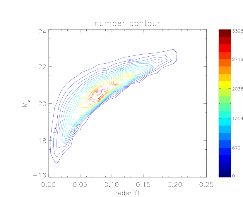
Figure 3: The restframe $r$-band Petrosian absolute magnitude vs. the redshift of the galaxies in the parent sample, where fracDeV_r ranges  from $0-0.1$. The lower absolute magnitude limit corresponds to an apparent magnitude of $17.77$ mag.

To continue with the sample selection we plot the number distribution of the axis ratio of the galaxies ($b/a$) in Figure 2(a) to 2(c). Solely based on redshift cuts and without additional magnitude cuts on top of the survey magnitude limits, we see that at lower redshifts (Figure 2(a), $z$  = $0.03-0.04$) the face-on galaxies are relatively under-sampled. Conversely, at higher redshifts (Figure 2(c), $z$ = $0.1-0.11$) the edge-on galaxies are relatively under-sampled. The upper and lower absolute magnitude limits are illustrated in Figure 3, as a function of redshift. As the SDSS spectroscopic sample is flux-limited ($r$-band Petrosian apparent magnitude brighter than $17.77$ mag), we deduce that the lack of edge-on galaxies at higher redshifts is due to the dropping out of the survey apparent magnitude limit for those highly inclined objects. At the redshift of 0.1, the highly inclined objects that are dropped out of the flux-limited survey would be, as inferred from Figure 3, intrinsically dimmer than $\approx~{}$-20. Conversely, the lack of face-on galaxies at lower redshifts is expected to be related to the interplay among all of the selection biases described previously, causing more edge-on systems to be picked.

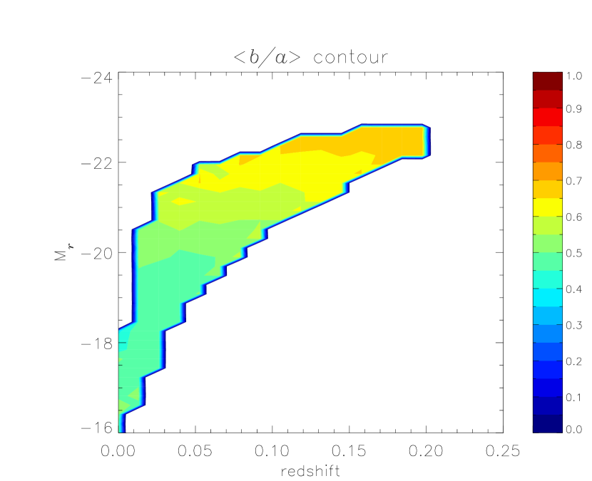
Figure 4: The average inclination of the galaxies (parent sample, fracDeV_r = $0-0.1$), plotted in the plane of $M_{r}$ vs. redshift. The corresponding number distribution is shown in Figure 3.

To understand further this result, we calculate the average inclination of the galaxies, plotted in the plane of $M_{r}$ vs. redshift (Figure 4). Only galaxies at $z\approx$ $0.065-0.075$ show an average inclination of $\approx$ 0.5, consistent with the expected average inclination of a random sample of galaxies that is unbiased against inclination and the range of the inclination being within 0 and 1. This consistency, we note, does not prove that those galaxies are free of any selection bias. One such indication is that the average b/a  value for brighter galaxies (brighter than M${}_{r}\approx~{}$-21) is not 0.5, but 0.65. This bias, however, does not affect the average luminosity in each of the composite spectra, because the average luminosity is heavily weighted towards the characteristic luminosity of a galaxy sample and less sensitive to the number of the bright-end objects. Besides, our lower absolute magnitude limit, -19.5, is dimmer than the characteristic magnitudes (the median $M_{r}$ ranged from -20.1 to -20.4 for b/a from 0.1 to 1.0 for galaxies at $z=$ $0.065-0.075$  in Figure 4), meaning that the characteristic luminosity is included in the luminosity distribution.

Because the $z=$ $0.065-0.075$ sample is mostly flat in terms of its inclination distribution (Figure 2(b)), the relatively small number of nearly edge-on ($b/a=0-0.1$) and nearly face-on ($b/a=0.9-1$) galaxies in Figure 2(b) is interpreted to be physical. Discussed by other authors (e.g., Shao et al., 2007; Unterborn & Ryden, 2008), in an unbiased sample the lack of exactly or nearly face-on galaxies is due to intrinsic ellipticity of the galaxies (on average $\epsilon=1-b/a=0.16$ in the SDSS disk galaxies, Ryden, 2004), and the lack of exactly or nearly edge-on galaxies is due to intrinsic thickness of the galaxy disks. Another factor that may come into play is that the axis ratio b/a may not be a pure inclination measurement of the disk component only, but of the combined bulge+disk systems which are subjected to the seeing effect. This factor could explain, e.g., the lack of edge-on galaxies. In the following, we confine ourselves to the galaxies located at redshift $0.065-0.075$, with a corresponding survey absolute magnitude limits of $\approx$ -19.5 to -22 mag in the $r$ band.

Finally, only spectroscopically-classified star-forming galaxies are considered, where narrow-line active galactic nuclei are removed from the sample through the line ratios [O III]/H$\beta$  vs. [N II]/H$\alpha$  according to the calibration by Kewley et al. (2006). In doing so the origin of the emission lines of the galaxies considered in the later session, e.g., the Balmer decrement (H$\alpha$/H$\beta$), is well constrained – arise from the H II region that is excited by the O/B stars. We take the equivalent widths (EW’s) of these emission lines as those measured by the SDSS, and add a constant restframe stellar absorption of 1.3 Å  to each of the Balmer lines (Hopkins et al., 2003; Miller et al., 2003). Each of the involved emission lines is required to be larger than 0.7 Å  in the restframe EW, and is of at least 2$\sigma$ detection. These selection criteria provide higher confidence to the Balmer decrement measurements that are performed in §5. Composite spectra are constructed in several bins of inclination: $b/a=0.1-0.2,0.2-0.3,0.3-0.4,0.4-0.5,0.5-0.6,0.6-0.7,0.7-0.8,0.8-0.9,$ and $0.9-1.0$. The bin $0.0-1.0$ is dropped in the subsequent analysis because of the limited number of galaxies (Table  1).

2.2 Fraction of Galaxy Light through Spectroscopic Fiber

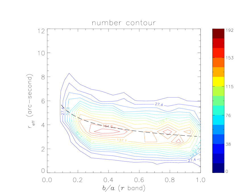
Figure 5: The $r$-band apparent half-light radius, ${r_{\rm eff}}^{b/a}$, as a function of inclination of the galaxies in the parent sample that lie in a fracDeV_r range  from $0-0.1$. The dashed line is the best-fit functional form ${\log}_{10}\left({r_{\rm eff}}^{b/a}\right)={\log}_{10}\left({r_{\rm eff}}^{1}\right)-0.26\,{\log}_{10}\left(b/a\right)$.

The apparent half-light radius of the star-forming disk galaxies is found to increase with the galaxy inclination, as shown in Figure 5. Similar to Maller et al. (2009), the relation in our galaxies can be described by

$${\log}_{10}\left({r_{\rm eff}}^{b/a}\right)={\log}_{10}\left({r_{\rm eff}}^{1}\right)-\beta_{r}\,{\log}_{10}\left(b/a\right)\ ,$$ (1)

where ${r_{\rm eff}}^{b/a}$ is the apparent half-light radius of the inclined galaxies, and ${r_{\rm eff}}^{1}$ is the value of the face-on galaxies. Through a linear least-square fit, the best-fit coefficient in the $r$ band, $\beta_{r}$, is found to be $0.26\pm 0.01$. This value agrees fairly well with that from Maller et al. (2009), who found $\beta_{r}=0.2$ for a different sample of nearby SDSS disk galaxies which also showed inclination dependency in their observed properties. The larger apparent half-light radius in the more inclined disk galaxies was seen also in Huizinga & van Albada (1992) and Möllenhoff et al. (2006), respectively in an independent galaxy sample and in a model for galaxy spectra. The adoption of the relation in Eqn. 1 is physically motivated. Its origin is presumably related to the extinction radial gradient in the galaxies, so that in the inclined galaxies the central region dims by a greater degree than the outer regions, resulting in an increased apparent half-light radius. This explanation is consistent with what we found later (see Figure 8), that dust is present at least in the disk galaxies, and more so for the more inclined galaxies.

Correcting the half-light radius of each galaxy by using Eqn. 1, the sample-average ratio between the radius of the SDSS spectroscopic fiber (a constant $r_{\rm fiber}$$=1.5$″) and the face-on $r_{\rm eff}$ (i.e., $r_{\rm fiber}$/$r_{\rm eff}$¹) is calculated to be approximately 0.45. This ratio stays fairly constant with the galaxy inclination, implying that a similar fraction of the full galaxy light is measured in the spectra of various inclinations.

3 Inclination Dependency of Disk Composite Spectrum

A composite spectrum of the disk galaxies is constructed in each of the bins of inclination. The flux density ($f_{\lambda}$) of each disk galaxy spectrum is converted to luminosity density ($L_{\lambda}$) by multiplying with the standard factor $4\pi d_{L}^{2}$, where $d_{L}$ is the luminosity distance of the galaxy, so that a fair comparison among the composites can be undertaken regardless of the redshift of the galaxies. This importance was also pointed out in Burstein et al. (1991). We use the concordance cosmological parameters in calculating $d_{L}$. The flux density of a composite spectrum in each wavelength bin is taken to be the geometric mean of those from the contributing spectra, which preserves the average of the steepness of the spectral slopes in a sample (e.g., Vanden Berk et al., 2001), and is effective in removing noisy data. Following the SDSS convention, the composite spectra are expressed in vacuum wavelengths, and are rebinned into $3700-8000$ Å  with a spectral resolution of 70 km s^-1 per wavelength bin.

The comparison between the composite spectra of face-on $(b/a=0.9-1.0)$ and edge-on $(b/a=0.1-0.2)$ disk galaxies is shown in Figure 6 and 7. A marked difference is seen in the luminosity and the slope between the continua, as such the inclined galaxies show a lower luminosity and a smaller slope in the continuum. The effect is in agreement with the usual power-law wavelength dependence in extinction curves (e.g., Calzetti et al., 1994).

4 Continuum Extinction in $g,r,i$ bands

4.1 Relative Continuum Extinction

Assuming the inclination dependency in the composite spectra is mainly due to extinction in the samples of the galaxies, we calculate the extinction of the inclined disk at the filter band $x$, $A_{x}(b/a)$ (mag), by comparing the inclined with face-on luminosity ($L_{x}(b/a)$ and $L_{x}(1)$) derived from the composite spectra according to

$$A_{x}(b/a)-A_{x}(1)=-2.5\log_{10}\left[L_{x}(b/a)/L_{x}(1)\right]\ ,$$ (2)

where $A_{x}(1)$ is the face-on extinction. The corresponding relative optical depth ($\tau_{x}(b/a)-\tau_{x}(1)$) can be obtained by dividing the extinction with the factor $2.5\,\log_{10}(e)$ or $1.086$. Although one can get only the inclined extinction relative to the face-on value but not both individually, the advantage of this approach is its being empirical. Throughout the paper, we denote the face-on inclinations to be $b/a=1$ for simplicity, where the highest inclinations are in fact $0.94\pm 0.02$ for our sample (Table 2).

The broad-band luminosity is derived by convolving a composite spectrum with a given filter response curve. To focus on the extinction in the stellar populations instead of other components such as the H II regions, the flux contribution from any emission line to the synthetic magnitudes are excluded. To make sure the continuum extinction is not biased by the continuum estimation method, we use and compare two independent approaches: (1) an empirical sliding window approach (2) a Bayesian approach based on a stellar population model.

In the sliding window approach, the continuum luminosity density at a given restframe wavelength is estimated to be the average luminosity density between the 40th and 60th percentiles of the sample distribution of the contributing luminosity densities, which are in turn taken from within $\pm 150$ wavelength bins (in the spectral resolution of 70 km s^-1 per bin) around the centered wavelength. The emission lines are masked out within a constant wavelength window of $\pm 280$ km s^-1, utilizing the line list in Table 30 of Stoughton et al. (2002).

In the Bayesian approach, the method outlined in Kaviraj et al. (2007) is adopted. We use the Bruzual & Charlot (2003) high-resolution model (1 Å resolution in the restframe wavelengths considered in this work) to determine the integrated stellar light of each composite spectrum, and the extinction model by Calzetti et al. (2000) for the dust reddening. The star formation history is characterized by an exponential declining star formation rate defined by an e-folding time, and the model parameters are, the age of the oldest stars: $1-13.7$ Gyr, the stellar metallicity ($Z$): $0.0004-0.05$, the e-folding time: $1-15$ Gyr, and the nebular gas emission-line reddening: $0-0.8$ mag.

For space saving, not all of the results using both continuum estimation methods are presented. However, we stress that there is no substantial difference detected in the continuum extinction values between both approach. For unity, we present and discuss our results in this work based on the Bayesian continuum estimation, unless otherwise specified. One significant advantage of the Bayesian approach is in the Balmer-line measurements, as will be shown in §5, where the flux contribution from the underlying stellar absorption is represented automatically by using the best-fit stellar population model spectrum.

In Figure 8 we see that the relative $g$-band extinction $A_{g}(b/a)-A_{g}(1)$ increases with the inclination of the galaxies. The relative extinctions for the volume-limited sample are given in Table 2. In the highly inclined objects ($b/a=0.26\pm 0.03$) $A_{g}(b/a)-A_{g}(1)$ is $\approx{0.4}$ mag, $A_{r}(b/a)-A_{r}(1)$ is $\approx{0.2}$ mag, and $A_{i}(b/a)-A_{i}(1)$ is $\approx{0.1}$ mag.

4.2 Empirical Extinction Model

To extrapolate the relative extinction to even higher inclination values where no result is available, empirical models are used. The $\log(b/a)$ model (de Vaucouleurs et al., 1991; Bottinelli et al., 1995; Tully et al., 1998) is

$$A_{x}(b/a)-A_{x}(1)=-\gamma_{x}\,\log_{10}\left(b/a\right)\ .$$ (3)

The best-fit model is drawn in Figure 8. As found also by Unterborn & Ryden (2008), the actual dependence is found here to be steeper than that described by the $\log(b/a)$ model. Instead, we found the following

$$A_{x}(b/a)-A_{x}(1)=\eta_{x}\,\log_{10}^{4}\left(b/a\right)$$ (4)

provides a better fit to our result. This choice is purely empirical, as a physically motivated model depends on knowledge of the actual distribution of stars and dust in a galaxy. In the $g$ band, the best-fit $\eta_{g}=$1.2 mag. This value gives a relative extinction of 1.2 mag for highly inclined galaxies with $b/a=0.1$, agrees with those from the previous studies (Shao et al., 2007; Maller et al., 2009) at the same inclination, both being $\stackrel{{\scriptstyle>}}{{{}_{\sim}}}{1}$ mag in the $g$ band.

4.3 Theoretical Extinction Model: Face-On Extinction

To derive the face-on ($b/a=1$) extinction, the inclination-dependent continuum extinction is fitted with theoretical models which describe the distributions of stars and dust in individual galaxies. The screen model is

$$A_{x}(b/a)=A_{x}(1)/(b/a)\ .$$ (5)

In this scenario, the absorbing layer of material is located above the stars like a screen. This choice is motivated by the study of Shao et al. (2007) where the authors found that the optical depth of inclined disk galaxies in the SDSS is proportional to the cosine of the inclination angle, which is in accord to the description by the screen model. Next, the slab model is considered

$$A_{x}(b/a)=-2.5\,{\log}_{10}{\left[{\frac{b/a}{\tau_{x}(1)}}\,\left(1-e^{-\tau_{x}(1)/(b/a)}\right)\right]}\ ,$$ (6)

for which the stars and the dust are mixed uniformly in a slab. Finally, the sandwich model is

$$A_{x}(b/a) = -2.5\,{\log}_{10}{\left[\frac{1-\zeta}{2}\left(1+e^{-\tau_{x}(1)/(b/a)}\right)\right.}$$ (8)

$$+\left.\frac{\zeta*(b/a)}{\tau_{x}(1)}\left(1-e^{-\tau_{x}(1)/(b/a)}\right)\right]\ ,$$

for which a layer of dust+stars mixture is sandwiched in-between two layers of stars. In these models the face-on extinction and the optical depth are respectively $A_{x}(1)$ and $\tau_{x}(1)$. The geometry of these models are illustrated in detail in Disney et al. (1989). Our model choice for dust+stars is non-exhaustive, there are other models in the literature which address, e.g., the presence of clumped dust (e.g., Tuffs et al., 2004), which we plan to explore in the future.

The best-fit models are drawn in Figure 9. The corresponding best-fit face-on extinctions in the SDSS $g,r,i$ bands are given in Table 3. Among all models the screen model performs the least satisfactory, whereas the slab and sandwich models perform similarly. The best-fit values of $A_{g}(1)$ are model-dependent, as pointed out also by Disney et al. (1989). The best-fit $A_{g}(1)$ however are similar in both the slab and sandwich models, $\sim{0.2}$ mag.

4.4 Extinction Curves in the Optical

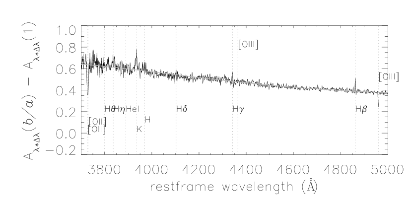
Figure 10: The extinction curve obtained by comparing the edge-on ($b/a=0.1-0.2$) with face-on ($b/a=0.9-1$) composite spectra, according to Eqn. 2. The gray line is the best-fit 3rd degree polynomial function on the emission-line excluded continuum. See Figure 11 for restframe wavelengths longer than 5000 Å.

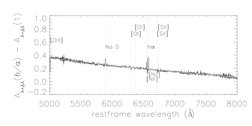
Figure 11: Continuation of Figure 10 to wavelengths $5000-8000$ Å.

The wavelength dependence of the relative extinction is obtained by comparing the inclined to face-on composite spectra. In the following discussions, the inclined spectrum is chosen to be that from the highest inclinations ($b/a=0.1-0.2$), the detailed inclination dependence of the relative extinction in the continuum can be obtained, e.g., by invoking the best-fit empirical or theoretical models (§4.2, §4.3). Within the restframe wavelength range $3700-8000$ Å, the relative extinction as a function of wavelength is calculated according to Eqn. 2, where the broad-band luminosity on the left-hand-side is now substituted by the luminosity density ($L_{\lambda}$) of the composite spectrum multiplied by the size of the wavelength bin ($\Delta{\lambda}$) at the concerned wavelength. The resultant extinction curve is shown in Figure 10 for $\lambda=3700-5000$ Å, and Figure 11 for $\lambda=5000-8000$ Å. Comparing the relative extinction in the lines and in the stellar continuum, the following cases can be visually identified:

$\dagger$

lines which exhibit relative extinction larger than that in the surrounding stellar continuum: Ca K and H absorptions, Na D$\lambda{5896}$ absorption, He I$\lambda{3889}$, H$\alpha$, H$\beta$, H$\gamma$, H$\delta$  emissions, [N II]$\lambda{6550}$ and $\lambda{6585}$ emissions

$\dagger$

lines which exhibit relative extinction smaller than that in the surrounding stellar continuum: [O III]$\lambda{4960}$ and $\lambda{5008}$, [O II]$\lambda{3727}$ and $\lambda{3730}$ and [O I]$\lambda{6302}$ emissions

$\dagger$

lines which exhibit relative extinction similar to that in the surrounding stellar continuum: [S II]$\lambda{6718}$ and $\lambda{6733}$ emissions

$\dagger$

uncertain due to small line strength in the composite spectra: H$\eta$, H$\theta$  emissions, [O III]$\lambda{4364}$, [O I]$\lambda{6366}$ emissions

These lines are all present in the face-on composite disk spectra, albeit in the last case the line strengths in the composite spectra are too small for identification. It is intriguing to see that there is a variety of behaviors, in terms of the inclination-induced dust extinction among the emission/absorption lines, and their relation to the extinction in the stellar continuum. In particular, none of the oxygen forbidden emission lines shows larger relative extinction than in the stellar continuum. Besides, the relative extinction in the [O III]$\lambda{5008}$ is smaller than that in the H$\beta$, a little bit surprising if they are emitted from the same H II region. These results are expected to give us hints on the geometry of the dust in relation to the regions where these lines arise, and on the extinction mechanism (e.g., type of dust) on each of the elements. This analysis however is beyond the scope of this paper, and will be performed in a future work. In this work we focus only on the Balmer decrement, H$\alpha$/H$\beta$, commonly used for deriving the dust reddening in H II region within a emission-line galaxy, later in §5.

The wavelength-dependent relative extinction in the stellar continuum is next fitted by a polynomial function of the 3rd degree

$$A_{\lambda*\Delta\lambda}(b/a)-A_{\lambda*\Delta\lambda}(1)=\sum_{j=0}^{3}\,a_{j}\,{\tilde{\nu}}^{j}\ ,$$ (9)

where the wavenumber $\tilde{\nu}$ (i.e., inverse wavelength, $\tilde{\nu}=1/\lambda$) is in the unit of inverse micron, $\micron^{-1}$. The best-fit coefficients are given in Table 4.

Assuming the stellar population and dust properties of the edge-on galaxies are not specially different from those of the face-on galaxies, the combination of Eqn. 2 and Eqn. 9 can be used to correct against the effects of reddening and extinction in the observed continuum of an inclined star-forming disk galaxy.

5 Balmer Decrement

The reddening on the emissions from the H II regions such as the Balmer decrement (the intensity ratio between H$\alpha$  and H$\beta$) depends on the detailed geometry of the dust and the gas (e.g., Caplan & Deharveng, 1986). If the reddening induced by the galaxy inclination affects the emissions from the H II regions of the galaxy in a similar manner as the integrated light from the continuum-generating stars, the measured H$\alpha$/H$\beta$  ratio can in-principle depend on the inclination of a galaxy. We therefore explore the relationship between the Balmer decrement and the inclination-dependent continuum extinction.

The Balmer line ratio H$\alpha$/H$\beta$ provides a mean for characterizing the dust reddening in “normal” H II regions (case B recombination, $n_{e}=100$ cm^-3, $T_{e}=10,000$ K), because the line ratio is fairly in-sensitive to the electron temperature (see Table 4.4 of Osterbrock, 1989). In measuring the EW of a Balmer line, we fit to the continuum-subtracted composite spectrum a single Gaussian function. In measuring the uncertainty in an EW, the following steps are performed. Firstly, the uncertainty in the luminosity densities of the stellar continuum in each composite is calculated by using ${\delta{L_{\lambda}^{c}}/{L_{\lambda}^{c}}}={\delta{L_{\lambda}}/{L_{\lambda}}}$, where $\delta$ denotes the uncertainty of a quantity. The uncertainty in each Balmer EW is calculated to be $\sum_{\lambda_{R}}{\delta{(L_{\lambda}-L_{\lambda}^{c})}/{L_{\lambda}^{c}}}\,d\lambda$, where $\lambda_{R}$ is the region of influence of the emission lines, taken to be around the line center, $\pm 280$ km s^-1  and $\pm 200$ km s^-1, respectively for the emission lines H$\alpha$ and H$\beta$. Finally, the uncertainty in the H$\alpha$/H$\beta$ is propagated by using $(\textrm{H}\alpha/\textrm{H}\beta)\,\sqrt{(}(\delta\textrm{H}\beta/\textrm{H}\beta)^{2}+(\delta\textrm{H}\alpha/\textrm{H}\alpha)^{2})$.

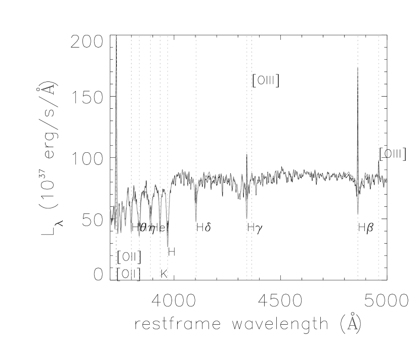
Figure 12: The face-on ($b/a=0.9-1.0$) composite spectrum (black) and the best-fit stellar continuum using the Bayesian approach (gray), in the vicinity of the H$\beta$.

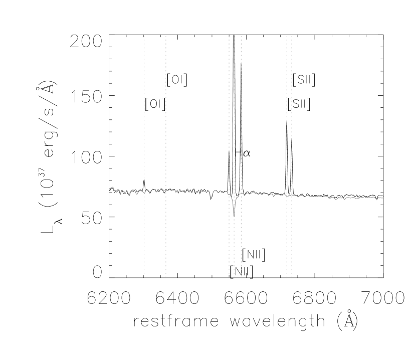
Figure 13: The face-on ($b/a=0.9-1.0$) composite spectrum (black) and the best-fit stellar continuum using the Bayesian approach (gray), in the vicinity of the H$\alpha$.

Examples of the best-fit stellar continua in the vicinity of H$\beta$ and H$\alpha$  emissions are shown respectively in Figure 12 and Figure 13. Using the Bruzual and Charlot stellar population model and the Calzetti dust model, in the Bayesian approach the underlying stellar absorption lines are represented obviously in the best-fit continuum.

The inclination dependency of the H$\alpha$ and H$\beta$ EW’s is shown respectively in Figure 14 and 15, for the sliding window approach (left figures) and the Bayesian approach (right figures). The offset between both approaches is $\approx~{}{7}$ Å  for the H$\alpha$, and $\approx~{}{4}$ Å  for the H$\beta$. If the stellar absorptions are not taken into account as in the sliding window approach, the H$\alpha$/H$\beta$ would be mis-taken to be approximately a factor of 1.5 larger for our galaxies.

The inclination dependency of the measured H$\alpha$/H$\beta$ is shown in Figure 16, using the geometric mean spectra. The Balmer decrements are also calculated in the median spectra, shown in Figure 17, which is expected to preserve the relative line strengths (Vanden Berk et al., 2001). The H$\alpha$/H$\beta$ calculated using the median composite spectra are consistent with those obtained by using the geometric composite spectra. Both plots show that the H$\alpha$/H$\beta$  remains fairly constant with inclination – a different behavior from the stellar continuum extinction, which shows inclination dependency.

5.1 Reddening in H II Region vs. in Continuum-Generating Stars

We adopt the Balmer optical depth ($\tau^{l}_{\rm B}$, Calzetti et al., 1994), a measure of the dust reddening from the measured Balmer line ratio, as follows

$$\tau^{l}_{\rm B}=\log_{e}{\left(\frac{\textrm{H}\alpha/\textrm{H}\beta}{(\textrm{H}\alpha/\textrm{H}\beta)^{T}}\right)}\ .$$ (10)

The superscript $l$ was used by the authors to indicate that $\tau^{l}_{\rm B}$ derived from the emission lines H$\alpha$  and H$\beta$. The ratio $(\textrm{H}\alpha/\textrm{H}\beta)^{T}$ is the un-reddened Balmer decrement, taken to be the theoretical value, 2.86 (Caplan & Deharveng, 1986; Osterbrock, 1989) in this work, which is accurate to 1 % for $T_{e}=5,000-20,000$ K.

The Balmer optical depth vs. the inclination-dependent $g$-band stellar continuum optical depth ($\tau_{g}(b/a)$) is shown in Figure 18. The face-on optical depths ($\tau_{g}(1)$) are taken to be the best-fit values in the slab model  (Table 3). One relation is evident, that most of the points of small optical depths deviate by more than 1$\sigma$  sample scatter from the one-to-one relationship (the dashed line in Figure 18, where $\tau^{l}_{\rm B}=\tau_{g}(b/a)$), because $\tau^{l}_{\rm B}$ is relatively larger.

Next, the color excess obtained from the Balmer decrement is compared with that derived from the inclination-dependent continuum extinction. The intrinsic color excess derived from the Balmer decrement, labeled as ${E(B-V)}_{\rm Balmer}$   in this work, is related to the Balmer optical depth as follows (Calzetti et al., 1994)

$${E(B-V)}_{\rm Balmer}\approx 0.935\,\tau^{l}_{\rm B}\ .$$ (11)

The color excess in stars, ${E(B-V)}_{\rm stars}^{b/a}$, is calculated at a given inclination, $b/a$, by using

$${E(B-V)}_{\rm stars}^{b/a} = {(B-V)}_{\rm stars}^{b/a}-{(B-V)}_{\rm stars}^{\rm 0}$$ (12)

$$= A_{B}(b/a)-A_{V}(b/a)\ ,$$ (13)

where ${(B-V)}_{\rm stars}^{\rm 0}$ is the intrinsic stellar Johnson $B-V$ color of the stars, and ${(B-V)}_{\rm stars}^{b/a}$ is the reddened color due to the inclination effect. Looking at Eqn. 13 and Eqn. 2, the value of ${E(B-V)}_{\rm stars}^{b/a}$ can be calculated by using the empirical continuum extinctions $A_{B}(b/a)-A_{B}(1)$ and $A_{V}(b/a)-A_{V}(1)$, obtained in a similar fashion as in §4 by using the Johnson filter response curves. The face-on extinctions $A_{B}(1)$ and $A_{V}(1)$ are taken to be those from the slab model (Table 3). The ${E(B-V)}_{\rm stars}$  depends weakly on the model, because the model-dependency of the face-on extinctions in the two photometric bands is reduced in the subtraction when calculating ${E(B-V)}_{\rm stars}$. If the face-on extinction derived by the screen model is used instead, the points are to be moved toward left horizontally by 0.1 unit  in the plot (not shown), which do not affect the above results qualitatively.

The comparison between the Balmer-line and stellar continuum color excess is plotted in Figure 19. Most of the points deviate by more than 1$\sigma$ uncertainty from the “uniform interstellar extinction” line (Caplan & Deharveng, 1986), the dashed line in each sub-figure which indicates the presence of uniform interstellar extinction in every galaxy of the sample. And, the Balmer-line color excess is larger than the continuum color excess.

If we assume the color excesses are related so that ${E(B-V)}_{\rm stars}^{b/a}=c\,{E(B-V)}_{\rm Balmer}$, where $c$ is a constant, then we find

$${E(B-V)}_{\rm stars}^{b/a}=\left(0.23\pm 0.20\right)\,{E(B-V)}_{\rm Balmer}$$ (14)

for our sample. The constant is calculated using $c=\sum{E(B-V)}_{\rm stars}^{b/a}\,/\sum{E(B-V)}_{\rm Balmer}$, over all of the inclinations. The result ${E(B-V)}_{\rm Balmer}>{E(B-V)}_{\rm stars}^{b/a}$ agrees qualitatively with that by Calzetti et al. (2000) (their Eqn. 3, with a proportional constant of $0.44\pm 0.03$), although our proportional constant is approximately a factor of 2 lower, both values are consistent to 1$\sigma$  uncertainty. We discuss these results in §6.1.

6 Discussion & Summary

6.1 Spatially Non-uniform Interstellar Extinction

Our study shows the lack of a correlation between the Balmer optical depth and the continuum optical depth, and between the Balmer-line color excess and the continuum color excess. If every galaxy of the sample exhibits uniform interstellar extinction, one would expect ${E(B-V)}_{\rm Balmer}={E(B-V)}_{\rm stars}$ at a given inclination. These results are likely the manifestations of the non-uniform interstellar extinction in at least some of the galaxies in each of the sample. Found also earlier in the H II regions in the Large Magellanic Cloud (Caplan & Deharveng, 1986), it describes the situation where the optical thickness of the dust in front of the light-emitting regions is not the same across the area being observed on a galaxy. Combining with the factor in which the spatial distribution of the star-forming H II regions can be different (e.g., clumped and/or patchy) from that of the continuum-generating stars (e.g., low mass stars), the measured extinctions in the stars and in the H II regions thus can be different.

6.2 Summary

Our study provides a determination of the wavelength-dependent extinction in a large and well-defined sample of star-forming disk galaxies, independent from previous works in the literature. We found that both the luminosity and the steepness of the spectral slope of the composite spectra decrease (i.e., extinguished and reddened) with the inclination of disk galaxies, in a volume-limited sample in $z=$ $0.065-0.075$ and $M_{r}=$ -19.5 to -22 mag  from the SDSS DR5. Assuming this effect is mainly due to intrinsic extinction in the galaxies, in the SDSS $g$-band the inclined relative to face-on continuum extinctions are found empirically to be 1.2 mag for highly inclined objects ($b/a=$ 0.1). The derived face-on extinction is model dependent, nonetheless with both the slab and sandwich models giving 0.2 mag  in the $g$ band. The extinction curve shows a variety of extinction, in both the sign and the amplitude, for emission/absorption lines relative to the stellar continuum. The parameterized extinction curves allow for correcting the observed galaxy continuum against the inclination effect.

The H$\alpha$/H$\beta$ does not show dependence with the inclination, and remain fairly constant. This inclination dependency is different from that in the stellar continuum, suggesting the mechanism and/or the dust configuration responsible for the reddening are different in the H II region and in the continuum-generating stars. The color excess ${E(B-V)}_{\rm Balmer}>{E(B-V)}_{\rm stars}$ at most inclinations, rather than the equality of both. From this we conclude that at least some of the galaxies exhibit the spatially non-uniform interstellar extinction, possibly caused by the presence of the clumped dust in the vicinity of the H II region in the galaxies.

The next step is to correct for the observed properties with existing parameter-inclination relations (e.g., Shao et al., 2007; Unterborn & Ryden, 2008; Driver et al., 2008; Maller et al., 2009, and this work), re-select the galaxies, and repeat the analysis. The convergence of the parameter-inclination relations is essential for ensuring their correctness. This approach is with reference with Driver et al. (2007), who developed an iterative approach to derive cosmic mass densities of the bulge, disk and dust components due to disk galaxies, and found converged extinction-inclination relations for those galaxies.

Our study also raises several interesting questions. For example, does the variation of extinction as a function of inclination from our current empirical measurement agree with that by other approaches, such as stellar population synthesis modeling? Can we build a model to describe the distributions of dust, gas, stars and line-emitting regions, that would explain the relative amount of extinction in the emission/absorption lines and the stellar continuum, to meet the extinction curve? Can we apply the current analysis to other galaxy types? What is the effect of galaxy inclination on photometric redshift, given that the inclination causes a reddening to the colors of a galaxy? We will leave these studies to future papers. Because our sample selection is well defined in a publicly available data set, works can be carried out easily even by other researchers in exploring any secondary factors that may affect the extinction in the galaxies.

7 Acknowledgments

CWY thanks Reynier F. Peletier for discussions on extinction in galaxies. We thank the referee for informative and insightful comments, particularly on the sample selection. We acknowledge support through grants from the W.M. Keck Foundation and the Gordon and Betty Moore Foundation, to establish a program of data-intensive science at to the Johns Hopkins University. IC and LD acknowledge support from NKTH:Polanyi and KCKHA005 grants.

This research has made use of data obtained from or software provided by the US National Virtual Observatory, which is sponsored by the National Science Foundation.

Funding for the SDSS and SDSS-II has been provided by the Alfred P. Sloan Foundation, the Participating Institutions, the National Science Foundation, the U.S. Department of Energy, the National Aeronautics and Space Administration, the Japanese Monbukagakusho, the Max Planck Society, and the Higher Education Funding Council for England. The SDSS Web Site is http://www.sdss.org/.

The SDSS is managed by the Astrophysical Research Consortium for the Participating Institutions. The Participating Institutions are the American Museum of Natural History, Astrophysical Institute Potsdam, University of Basel, University of Cambridge, Case Western Reserve University, University of Chicago, Drexel University, Fermilab, the Institute for Advanced Study, the Japan Participation Group, Johns Hopkins University, the Joint Institute for Nuclear Astrophysics, the Kavli Institute for Particle Astrophysics and Cosmology, the Korean Scientist Group, the Chinese Academy of Sciences (LAMOST), Los Alamos National Laboratory, the Max-Planck-Institute for Astronomy (MPIA), the Max-Planck-Institute for Astrophysics (MPA), New Mexico State University, Ohio State University, University of Pittsburgh, University of Portsmouth, Princeton University, the United States Naval Observatory, and the University of Washington.

3

(a) $z$ = $0.03-0.04$.

(b) $z$ = $0.065-0.075$.

(c) $z$ = $0.1-0.11$.

Figure 2: The number distribution of the axis ratio ($b/a$) of the galaxies in our parent sample in the range fracDeV_r  = $0-0.1$, at three different slices of redshift. The narrowest in the redshifts is designed for the purpose of generating volume-limited samples. Without additional magnitude cuts, we see that at lower redshifts (Figure 2(a)) the face-on galaxies are relatively under-sampled. Conversely, at higher redshifts (Figure 2(c)) the edge-on galaxies are relatively under-sampled.

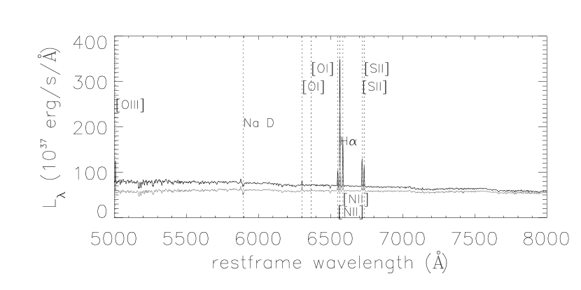
Figure 7: Continuation of Figure 6 to wavelengths $5000-8000$ Å.

Figure 8: Dependency of the $g$-band relative extinction in the disk galaxies on their inclination, for the volume-limited sample. The best-fit empirical models are the log model (dashed line), and the log⁴ model (dot-dot-dot-dashed line).

Figure 9: Dependency of the $g$-band relative extinction in the disk galaxies on their inclination, for the volume-limited sample. The best-fit theoretical models are the screen model (dotted line), the slab model (dashed line) and the sandwich model (dot-dot-dot-dashed line).

Figure 14: The inclination dependency of the H$\alpha$  equivalent width. The sliding window approach (left) and the Bayesian approach (right) are used respectively in estimating the stellar continuum in the composite spectra. The error bar is 1$\sigma$ statistical uncertainty for each parameter.

Figure 15: The inclination dependency of the H$\beta$ equivalent width. The sliding window approach (left) and the Bayesian approach (right) are used respectively in estimating the continuum in the composite spectra. The error bar is 1$\sigma$  statistical uncertainty for each parameter.

Figure 16: The inclination dependency of the Balmer decrement for the star-forming disk galaxies. The Bayesian approach is used in estimating the stellar continuum in the geometric composite spectra. The dashed line indicates the theoretical value of normal H II region. No obvious trend of H$\alpha$/H$\beta$  with inclination is found.

Figure 17: Same as Figure 16 but using the median composite spectra. The dashed line indicates the theoretical value of normal H II region. The Balmer decrement values are consistent to 1$\sigma$ uncertainty with those in Figure 16.

Figure 18: The Balmer optical depth vs. the $g$-band continuum optical depth. The error bar in each axis represents 1$\sigma$ uncertainty in the derived parameter. The dashed line indicates the locus if both optical depths are the same.

Figure 19: The comparison between the color excess derived from the Balmer decrement and from the inclination-dependent extinction in the stellar continuum, respectively. The error bar in each axis represents 1$\sigma$ uncertainty in the derived parameter. The dashed line indicates the locus if every galaxy in the sample exhibits uniform interstellar extinction, where ${E(B-V)}_{\rm Balmer}={E(B-V)}_{\rm stars}$ at a given inclination.

Table 1: Number of star-forming disk galaxy spectra in the volume-limited sample.

$b/a$	number
$0.94\pm 0.03$	387
$0.75\pm 0.03$	615
$0.65\pm 0.03$	625
$0.55\pm 0.03$	621
$0.45\pm 0.03$	678
$0.35\pm 0.03$	784
$0.25\pm 0.03$	684
$0.17\pm 0.02$	214
$0.09\pm 0.00$	2

Table 2: Relative extinction in disk galaxies as a function of inclination, in SDSS $g,r,i$ bands.

$b/a$	$A_{g}(b/a)-A_{g}(1)$	$A_{r}(b/a)-A_{r}(1)$	$A_{i}(b/a)-A_{i}(1)$
$0.94\pm 0.03$	$0.00\pm 0.18$	$0.00\pm 0.12$	$0.00\pm 0.15$
$0.75\pm 0.03$	$-0.04\pm 0.18$	$-0.04\pm 0.12$	$-0.04\pm 0.15$
$0.65\pm 0.03$	$-0.05\pm 0.18$	$-0.05\pm 0.12$	$-0.05\pm 0.15$
$0.55\pm 0.03$	$-0.09\pm 0.18$	$-0.10\pm 0.12$	$-0.11\pm 0.15$
$0.45\pm 0.03$	$-0.05\pm 0.18$	$-0.09\pm 0.12$	$-0.11\pm 0.15$
$0.35\pm 0.03$	$-0.04\pm 0.18$	$-0.12\pm 0.12$	$-0.16\pm 0.15$
$0.25\pm 0.03$	$0.15\pm 0.18$	$0.02\pm 0.12$	$-0.06\pm 0.15$
$0.17\pm 0.02$	$0.41\pm 0.19$	$0.23\pm 0.13$	$0.11\pm 0.15$

Table 3: Best-fit face-on extinction of star-forming disk galaxies in SDSS $g$, $r$, $i$ bands.

model	$A_{g}(1)$	reduced $\chi^{2}$	$A_{r}(1)$	reduced $\chi^{2}$	$A_{i}(1)$	reduced $\chi^{2}$
screen	$0.06\pm 0.03$	0.36	$0.02\pm 0.02$	0.67	$-0.01\pm 0.02$	0.47
slab	$0.20\pm 0.11$	0.17	$0.09\pm 0.06$	0.47	$0.02\pm 0.07$	0.45
sandwich	$0.15\pm 0.05$	0.19	$0.14\pm 0.14$	0.53	$0.15\pm 0.18$	0.45

Table 4: Extinction curve in star-forming disk galaxies, parameterized with 3rd degree polynomial.

$a_{0}$	$a_{1}$	$a_{2}$	$a_{3}$	reduced $\chi^{2}$
$-0.554\pm 0.014$	$0.564\pm 0.023$	$-0.057\pm 0.012$	$0.003\pm 0.002$	0.15

References

- Bailin & Harris (2008) Bailin, J., & Harris, W. E. 2008, ApJ, 681, 225
- Beckman et al. (1996) Beckman, J. E., Peletier, R. F., Knapen, J. H., Corradi, R. L. M., & Gentet, L. J. 1996, ApJ, 467, 175
- Boselli & Gavazzi (1994) Boselli, A., & Gavazzi, G. 1994, A&A, 283, 12
- Bottinelli et al. (1995) Bottinelli, L., Gouguenheim, L., Paturel, G., & Teerikorpi, P. 1995, A&A, 296, 64
- Burstein et al. (1991) Burstein, D., Haynes, M. P., & Faber, M. 1991, Nature, 353, 515
- Bruzual & Charlot (2003) Bruzual, G., & Charlot, S. 2003, MNRAS, 344, 1000
- Calzetti et al. (1994) Calzetti, D., Kinney, A. L., & Storchi-Bergmann, T. 1994, ApJ, 429, 582
- Calzetti et al. (2000) Calzetti, D., Armus, L., Bohlin, R. C., Kinney, A. L., Koornneef, J., & Storchi-Bergmann, T. 2000, ApJ, 533, 682
- Caplan & Deharveng (1986) Caplan, J., & Deharveng, L. 1986, A&A, 155, 297
- Davies et al. (1993) Davies, J. I., Phillips, S., Boyce, P. J., & Disney, M. J. 1993, MNRAS, 260, 491
- Davies & Burstein (1995) Davies, J. I., & Burstein, D. 1995, NATO ASIC Proc. 469: The Opacity of Spiral Disks
- de Vaucouleurs et al. (1991) de Vaucouleurs, G., de Vaucouleurs, A., Corwin, H. G., Jr., Buta, R. J., Paturel, G., & Fouque, P. 1991, Volume 1-3, XII, 2069 pp. 7 figs.. Springer-Verlag Berlin Heidelberg New York,
- Disney et al. (1989) Disney, M., Davies, J., & Phillipps, S. 1989, MNRAS, 239, 939
- Driver et al. (2007) Driver, S. P., Popescu, C. C., Tuffs, R. J., Liske, J., Graham, A. W., Allen, P. D., & de Propris, R. 2007, MNRAS, 379, 1022
- Driver et al. (2008) Driver, S. P., Popescu, C. C., Tuffs, R. J., Graham, A. W., Liske, J., & Baldry, I. 2008, ApJ, 678, L101
- Elmegreen (1980) Elmegreen, D. M. 1980, ApJS, 43, 37
- Fukugita et al. (1996) Fukugita, M., Ichikawa, T., Gunn, J. E., Doi, M., Shimasaku, K., & Schneider, D. P. 1996, AJ, 111, 1748
- Giovanelli et al. (1994) Giovanelli, R., Haynes, M. P., Salzer, J. J., Wegner, G., da Costa, L. N., & Freudling, W. 1994, AJ, 107, 2036
- Gunn et al. (1998) Gunn, J. E., et al. 1998, AJ, 116, 3040
- Hogg et al. (2001) Hogg, D. W., Finkbeiner, D. P., Schlegel, D. J., & Gunn, J. E. 2001, AJ, 122, 2129
- Holmberg (1958) Holmberg, E. 1958, Meddelanden fran Lunds Astronomiska Observatorium Serie II, 136, 1
- Holwerda et al. (2007) Holwerda, B. W., Keel, W. C., & Bolton, A. 2007, AJ, 134, 2385
- Hopkins et al. (2003) Hopkins, A. M., et al. 2003, ApJ, 599, 971
- Huizinga & van Albada (1992) Huizinga, J. E., & van Albada, T. S. 1992, MNRAS, 254, 677
- Ivezić et al. (2004) Ivezić, Ž., et al. 2004, Astronomische Nachrichten, 325, 583
- Kauffmann et al. (2003) Kauffmann, G., et al. 2003, MNRAS, 341, 33
- Kaviraj et al. (2007) Kaviraj, S., Rey, S.-C., Rich, R. M., Yoon, S.-J., & Yi, S. K. 2007, MNRAS, 381, L74
- Kewley et al. (2006) Kewley, L. J., Groves, B., Kauffmann, G., & Heckman, T. 2006, MNRAS, 372, 961
- Lupton et al. (2001) Lupton, R., Gunn, J. E., Ivezić, Z., Knapp, G. R., & Kent, S. 2001, Astronomical Data Analysis Software and Systems X, 238, 269
- Maller et al. (2009) Maller, A. H., Berlind, A. A., Blanton, M. R., & Hogg, D. W. 2009, ApJ, 691, 394
- Miller et al. (2003) Miller, C. J., Nichol, R. C., Gómez, P. L., Hopkins, A. M., & Bernardi, M. 2003, ApJ, 597, 142
- Möllenhoff et al. (2006) Möllenhoff, C., Popescu, C. C., & Tuffs, R. J. 2006, A&A, 456, 941
- Osterbrock (1989) Osterbrock, D. E. 1989, Astrophysics of gaseous nebulae and active galactic nuclei, University Science Books.
- Pier et al. (2003) Pier, J. R., Munn, J. A., Hindsley, R. B., Hennessy, G. S., Kent, S. M., Lupton, R. H., & Ivezić, Ž. 2003, AJ, 125, 1559
- Ryden (2004) Ryden, B. S. 2004, ApJ, 601, 214
- Schlegel et al. (1998) Schlegel, D. J., Finkbeiner, D. P., & Davis, M. 1998, ApJ, 500, 525
- Shao et al. (2007) Shao, Z., Xiao, Q., Shen, S., Mo, H. J., Xia, X., & Deng, Z. 2007, ApJ, 659, 1159
- Shimasaku et al. (2001) Shimasaku, K., et al. 2001, AJ, 122, 1238
- Smith et al. (2002) Smith, J. A., et al. 2002, AJ, 123, 2121
- Stoughton et al. (2002) Stoughton, C., et al. 2002, AJ, 123, 485
- Strauss et al. (2002) Strauss, M. A., et al. 2002, AJ, 124, 1810
- Tuffs et al. (2004) Tuffs, R. J., Popescu, C. C., Völk, H. J., Kylafis, N. D., & Dopita, M. A. 2004, A&A, 419, 821
- Tully et al. (1998) Tully, R. B., Pierce, M. J., Huang, J.-S., Saunders, W., Verheijen, M. A. W., & Witchalls, P. L. 1998, AJ, 115, 2264
- Unterborn & Ryden (2008) Unterborn, C. T., & Ryden, B. S. 2008, ApJ, 687, 976
- Valentijn (1990) Valentijn, E. A. 1990, Nature, 346, 153
- Vanden Berk et al. (2001) Vanden Berk, D. E., et al. 2001, AJ, 122, 549
- White & Keel (1992) White, R. E., III, & Keel, W. C. 1992, Nature, 359, 129
- York et al. (2000) York, D. G., et al. 2000, AJ, 120, 1579
3