Improvements in the X-ray luminosity function and constraints on the Cosmological parameters from X-ray luminous clusters

We show how to improve constraints on $\Omega_{m}$, $\sigma_{8}$, and the dark-energy equation-of-state parameter, $w$, obtained by Mantz et al. (2008) from measurements of the X-ray luminosity function of galaxy clusters, namely MACS, the local BCS and the REFLEX galaxy cluster samples with luminosities $L>3\times 10^{44}$ erg/s in the 0.1–2.4 keV band. To this aim, we use Tinker et al. (2008) mass function instead of Jenkins et al. (2001) and the M-L relationship obtained from Del Popolo (2002) and Del Popolo et al. (2005). Using the same methods and priors of Mantz et al. (2008), we find, for a $\Lambda$CDM universe, $\Omega_{m}=0.28^{+0.05}_{-0.04}$ and $\sigma_{8}=0.78^{+0.04}_{-0.05}$ while the result of Mantz et al. (2008) gives less tight constraints $\Omega_{m}=0.28^{+0.11}_{-0.07}$ and $\sigma_{8}=0.78^{+0.11}_{-0.13}$. In the case of a $w$CDM model, we find $\Omega_{m}=0.27^{+0.07}_{-0.06}$, $\sigma_{8}=0.81^{+0.05}_{-0.06}$ and $w=-1.3^{+0.3}_{-0.4}$, while in Mantz et al. (2008) they are again less tight $\Omega_{m}=0.24^{+0.15}_{-0.07}$, $\sigma_{8}=0.85^{+0.13}_{-0.20}$ and $w=-1.4^{+0.4}_{-0.7}$. Combining the XLF analysis with the $f_{gas}$+CMB+SNIa data set results in the constraint $\Omega_{m}=0.269\pm 0.012$, $\sigma_{8}=0.81\pm 0.021$ and $w=-1.02\pm 0.04$, to be compared with Mantz et al. (2008), $\Omega_{m}=0.269\pm 0.016$, $\sigma_{8}=0.82\pm 0.03$ and $w=-1.02\pm 0.06$. The tightness of the last constraints obtained by Mantz et al. (2008), are fundamentally due to the tightness of the $f_{gas}$+CMB+SNIa constraints and not to their XLF analysis. Our findings, consistent with $w=-1$, lend additional support to the cosmological-constant model.

1 Introduction

Cluster of galaxies are the largest gravitationally-collapsed structures in the Universe. Even at the present epoch they are relatively rare, with only a few percent of galaxies being in clusters. In the hierarchical collapse scenario for structure formation in the universe, the number density of collapsed objects as a function of mass and cosmic time is a sensitive probe of cosmology. The galaxy clusters that occupy the high-mass tail of this population provide a powerful and relatively clean tool for cosmology, since their growth is predominantly determined by linear gravitational processes.

Starting in the 1990’s, analysis of massive clusters have consistently indicated low values of $\Omega_{m}$ (both from the baryonic fraction arguments (White et al. 1993) and measurements of the evolution in the cluster number density (Eke et al. 1998; Borgani et al. 2001) and low values of $\sigma_{8}$ (Henry & Arnaud 1991; Reiprich & Böringer 2002; Schuecker et al. 2003) –a result since then confirmed by cosmic microwave background (CMB) studies, cosmic shear, and other experiments (Spergel et al. 2007; Komatsu et al. 2008; Dunkley et al. 2008; Benjamin et al. 2007; Fu et al. 2008). For precision’s sake, cluster surveys in the local universe are particularly useful for constraining a combination of the matter density parameter $\Omega_{m}$ and the normalization of the power spectrum of density fluctuations. Following the evolution of the cluster space density over a large redshift baseline, one can break the degeneracy between $\sigma_{8}$ and $\Omega_{m}$ (Rosati et al. 2002). Recently, X-ray studies (Vikhlinin et al. 2009b) of the evolution of the cluster mass function at $z=$ 0-0.8 have convincingly demonstrated that the growth of cosmic structure has slowed down at $z<1$ due to the effects of dark energy, and these measurements have been used to improve the determination of the equation of state parameter. Although the quoted cosmological test is very powerful, there are two main problems in practical applications: first, theoretical predictions provide the number density of clusters of a given mass, while the mass itself is never the directly observed quantity. Second, a cluster sample is needed that spans a large-$z$ baseline and is based on model-independent selection criteria.

Determining the evolution of the space density of clusters requires counting the number of clusters of a given mass per unit volume at different redshifts. Therefore, three essential tools are required for its application as a cosmological test: (a) an efficient method to find clusters over a wide redshift range, (b) an observable estimator of the cluster mass, and (c) a method to compute the selection function or equivalently the survey volume within which clusters are found. Observations of clusters in the X-ray band provide an efficient and physically motivated method of identification, which fulfills the three requirements above. The X-ray luminosity, provides a very efficient method for identifying clusters down to a given X-ray flux limit and hence within a known survey volume for each luminosity $L_{x}$, which uniquely specifies the cluster selection, is also a good probe of the depth of the cluster gravitational potential. For these reasons most of the cosmological studies based on clusters have used X–ray -selected samples.

According to the three points quoted above, the recipe for constraining cosmological parameters by means of clusters is composed of three ingredients: 1) The predicted mass function of clusters, $n(M,z)$, as a function of cosmological parameters ($\sigma_{8}$, $\Omega_{m}$, $w$, etc.). 2) Sky surveys with well understood selection functions to find clusters, as well as a relation linking cluster mass with an observable. A successful solution to the former requirement has been to identify clusters by the X-ray emission produced by hot intracluster gas, notably using data from ROSAT. 3) A tight, well-determined scaling relation between survey observable (e.g. $L_{x}$) and mass, with minimal intrinsic scatter.

Early attempts to use evolution of the cluster mass function as a cosmological probe were limited by small sample sizes and either poor proxies for the cluster mass (e.g., the total X-ray flux) or inaccurate measurements (e.g. temperatures with large uncertainties)

Until some years ago the obtained results for $\Omega_{\rm m}$ were several times in disagreement. Study by different authors (Bahcall, Fan & Cen (1997), Bahcall & Fan (1998), Sadat, Blanchard & Oukbir (1998), Blanchard, Bartlett & Sadat (1998), Blanchard & Bartlett (1998), Eke et al. (1998), Viana & Liddle (1999), Reichart et al. (1999), Donahue & Voit 1999, Borgani et al. 2001) found values for $\Omega_{m}$ spanning the entire range of acceptable values: $0.2\leq\Omega_{\rm m}\leq 1$ (see Reichart et al. 1999). It is interesting to note that Viana & Liddle (1999) using the same data set as Eke et al. (1998) showed that uncertainties both in fitting local data and in the theoretical modeling could significantly change the final results: they found $\Omega_{\rm m}\simeq 0.75$ as a preferred value with a critical density model acceptable at $<90\%$ c.l. while Eke et al. (1998) found $\Omega_{\rm m}=0.45\pm 0.2$.

The reasons leading to the quoted discrepancies have been studied in several papers (Eke et al. 1998; Reichart et al. 1999; Donahue & Voit 1999; Borgani et al. 2001) and can be summarized as due to: 1) The inadequate approximation given by the mass function used (e.g., Bryan & Norman 1998). 2) Inadequacy in the structure formation as described by the spherical model leading to changes in the threshold parameter $\delta_{\rm c}$ (e.g., Governato et al. 1999). 3) Inadequacy in the M-T relation obtained from the virial theorem (see Voit & Donahue 1998; Del Popolo 2002). 4) Effects of cooling flows. 5) Determination of the X-ray cluster catalog’s selection function. 5) Missing high redshift clusters in the data used (e.g., the EMSS). 6) Evolution of the L-T relation (Voit & Donahue 1998). 7) The use of different best fitting procedures to get the constraints (Eke et al. 1998). 8) Other effects described in more recent papers (e.g., Mantz et al. 2008 (hereafter M08); Vikhlinin et al 2009b).

(a)  (b)

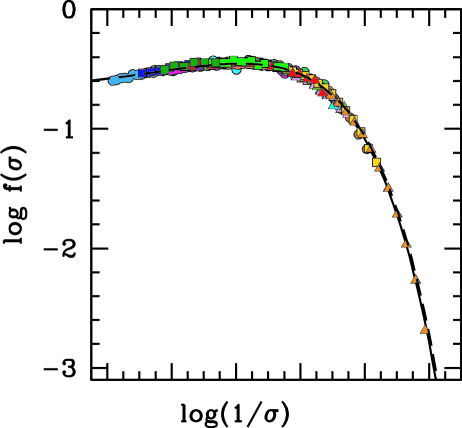
(b)  (b)

Figure 1: In Panel (a), the solid line represents the multiplicity function obtained in this paper, the short–dashed line the fitting formula proposed by Yahagi et al. (2004) (their Eq. 7), the dotted line the Sheth & Tormen (2002) (ST) multiplicity function, the long-dashed line the Jenkins et al. (2001) multiplicity function. The errorbars with open circles represent the run 140 of YNY, those with filled squares the case 70b, those with open squares the case 70a, those with filled circles the case 35b, those with crosses the case 35a. Panel (b). Mass function plotted in redshift-independent form. The measured $f(\sigma)$ from all simulations in Table 1 of Tinker et al. (2008). The solid line is the best fit function of equation (3) (Tinker et al. 2008). The dashed line the model in the present paper.

The situation with the cluster mass function data has been dramatically improved in the past years. A large sample of sufficiently massive clusters extending to $z\simeq 0.9$ has been derived from ROSAT PSPC pointed data covering 400 deg² (Burenin et al. 2007). Distant clusters from the 400d sample were then observed with Chandra, providing high-quality X-ray data and much more accurate total mass indicators (see Vikhlinin et al. 2009b). Chandra coverage has also become available for a complete sample of low-z clusters originally derived from the ROSAT All-Sky Survey (see Vikhlinin et al. 2009b). Results from deep Chandra pointings to a number of low-z clusters have significantly improved our knowledge of the outer cluster regions and provided a much more reliable calibration of the $M_{tot}$ vs. proxy relations than what was possible before. On the theoretical side, improved numerical simulations resulted in better understanding of measurement biases in the X-ray data analysis (Nagai et al. 2007; Rasia et al. 2006; Jeltema et al. 2007).

In the present paper, we want to show how tighter constraints can be obtained in M08 model improving the mass function adopted by them, and the scaling laws used (e.g., the M-T and M-L relationships). In this paper, we use the observed X-ray luminosity function to investigate two cosmological scenarios, assuming a spatially flat metric in both cases: the first includes dark energy in the form of a cosmological constant ($\Lambda$CDM); the second has dark energy with a constant equation-of-state parameter, w (wCDM). The theoretical background for this work is reviewed in Section 2. Section 3 presents the results and Section 4 the conclusions.

2 Theory

In the introduction, we discussed the ingredients needed in the recipe used to constrain cosmological parameters from X-ray observations. In this section, I derive an expression for the X-Ray luminosity function (XLF) (using now the mass function obtained in Del Popolo (2006a, b)) and M–T, L–T relations obtained in Del Popolo 2002, and Del Popolo et al. 2005, respectively) and then I set some constraints to $\Omega_{m}$, $\sigma_{8}$ and the dark–energy equation–of–state parameter $w$, by using the data (clusters) used in M08, namely MACS (Massive Cluster Survey), BCS (Brightest Cluster Sample), and REFLEX (ROSAT ESO FLUX LIMITED X-Ray SAMPLE). Following M08, the constraints are obtained from measurements of the X-Ray luminosity function of the quoted samples. The most straightforward mass -observable relation to complement these X–ray flux–limited surveys is the mass -X–ray luminosity relation. For sufficiently massive (hot) objects at the relevant redshifts, the conversion from X-ray flux to luminosity is approximately independent of temperature, in which case the luminosities can be estimated directly from the survey flux and the selection function is identical to the requirement of detection. A disadvantage is that there is a large scatter in cluster luminosities at fixed mass; however, sufficient data allow this scatter to be quantified empirically. More recently, a dramatic reduction in luminosity-mass scatter has been demonstrated when luminosities are measured excluding cluster centers (typically $r<0.15r_{500}$; Maughan 2007; Zhang et al. 2007). Alternative approaches use cluster temperature (Henry 2000; Seljak 2002; Pierpaoli et al. 2003; Henry 2004), gas fraction (Voevodkin & Vikhlinin 2004) or $Y_{X}$ parameter (Kravtsov et al. 2006) to achieve tighter mass -observable relations at the expense of reducing the size of the samples available for analysis. The need to quantify the selection function in terms of both X-ray flux and a second observable additionally complicates these efforts.

The first ingredient of the quoted recipe (i.e., mass function), used in M08 was the Jenkins et al. (2001) (hereafter J01) mass function. J01 wrote the mass function of galaxy clusters of mass $M$ at redshift $z$ as a ”universal function” of $\sigma^{-1}(M,z)$

$$f(\sigma^{-1})=\frac{M}{\rho_{m}}\frac{n(M,z)}{d\ln\sigma^{-1}}$$ (1)

which was fitted by

$$f(\sigma^{-1})=Ae^{(-|\ln\sigma^{-1}+B|^{\epsilon})}$$ (2)

for cosmological -constant models, with $A=0.316$, $B=0.67$, and $\epsilon=3.82$.

As shown in Del Popolo (2006a) and Del Popolo (2006b), the theoretical mass function obtained in the quoted papers is in better agreement with high resolution N-body simulations, namely Reed et al. 2003 (R03), Yahagi et al. (2004) (YNY), Warren et al. 2006 (W06), and Tinker et al. (2008) (see the following and Fig. 1b) (T08).

The mass function was calculated according to the model of Del Popolo (2006a, b). The multiplicity function, in the quoted model, is given by:

$$\nu f(\nu) = A_{1}\left(1+\frac{\beta_{1}g(\alpha_{1})}{\left(a\nu\right)^{\alpha_{1}}}+\frac{\beta_{2}g(\alpha_{2})}{\left(a\nu\right)^{\alpha_{2}}}+\frac{\beta_{3}g(\alpha_{3})}{\left(a\nu\right)^{\alpha_{3}}}\right)$$ (3)

$$\sqrt{\frac{a\nu}{2\pi}}e^{\{\frac{-a\nu}{2}\left[1+\frac{\beta_{1}}{\left(a\nu\right)^{\alpha_{1}}}+\frac{\beta_{2}}{\left(a\nu\right)^{\alpha_{2}}}+\frac{\beta_{3}}{\left(a\nu\right)^{\alpha_{3}}}\right]^{2}\}}$$

where

$$g(\alpha_{i}) = \mid 1-\alpha_{i}+\frac{\alpha_{i}(\alpha_{i}-1)}{2!}-...-$$ (4)

$$\frac{\alpha_{i}(\alpha_{i}-1)\cdot\cdot\cdot(\alpha_{i}-4)}{5!}\mid$$

where $i=1$ or 2, $\alpha_{1}=0.585$, $\beta_{1}=0.46$, $\alpha_{2}=0.5$ and $\beta_{2}=0.35$, $\alpha_{3}=0.4$ and $\beta_{3}=0.02$, $a=0.707$, and $A_{1}=1.2$ is the normalization constant.

The “multiplicity function” is correlated with the usual, more straightforwardly used, “mass function” as follows. Following Sheth & Tormen (2002) (hereafter ST) notation, if $f(M,\delta)dM$ denotes the fraction of mass that is contained in collapsed haloes that have mass in the range $M$-$M+dM$, at redshift $z$, and $\delta(z)$ is the redshift dependent overdensity, the associated “unconditional” mass function is:

$$n(M,\delta)dM=\frac{{\rho_{b}}}{M}f(M,\delta)dM$$ (5)

In Fig. 1a, we plot the multiplicity function obtained in this paper (simbols are described in the figure caption).

There are some differences between the quoted simulations and the J01 simulations. First, the multiplicity function of the present paper, similar to that of YNY, in the low-$\nu$ region of $\nu\leq 1$ systematically falls below the J01 functions. In this region the multiplicity function of the present paper is very close to that of YNY. Additionally, the numerical multiplicity functions (and that in Del Popolo 2006a,b) have an apparent peak at $\nu\simeq$ instead of the plateau that is seen in the J01 function. Similar differences are seen in the high-$\nu$ region. These differences between numerical multiplicity functions (R03; YNY; W05; Del Popolo 2006a,b) and J01, are however within 1–$\sigma$ error–bars, and so they are overall in agreement. The multiplicity function obtained in the present paper has a peak at $\nu\simeq 1$ as in YNY numerical multiplicity function, instead of a plateau as in the J01 function. Differences are observed also in the redshift evolution of the J01 mass function (Del Popolo 2006b). Summarizing the fitting formulas presented by J01 are accurate to $\simeq 10-20\%$ (Tinker et al. 2008 (T08)). In our model, the mass function that we used is given by Eq. (3), Eq.(4), and Eq(5) which is in perfect agreement with the T08 mass function, as shown in Fig. (1b). So, the accuracy of the mass function is, as in T08, of the order of $\simeq 5\%$ for $\Lambda$CDM models for the mass and redshift range of interest in this study. As a consequence, in this way the theoretical uncertainties in the mass function do not contribute significantly to the systematic error budget.

In Fig. 1b, I plot the mass function for all of our outputs in the $f(\sigma)-\ln(\sigma^{-1})$ plane. Large values of $\ln\sigma^{-1}$ correspond to rare haloes of high redshift and/or high mass, while small values of $\ln\sigma^{-1}$ describe haloes of low mass and redshift combinations. Fig. 1b shows the function $f(\sigma)$ measured for all simulations in Table 1 of T08, the solid line the fit to the data (namely T08 eq. 3) and the dashed line the model of the present paper.

As previously reported, one of the main problems of using the mass function to constrain cosmological parameter is that theoretical predictions provide the number density of clusters of a given mass, while the mass itself is never the directly observed quantity. One then needs relations connecting mass with other quantities more easily obtainable which can be used as a surrogate for cluster mass. Over the past decade, observations of clusters of galaxies (e.g. ROSAT, ASCA) have shown the existence of a correlation between the total gravitating mass of clusters, $M_{tot}$, their X-ray luminosity ($L_{X}$) and the temperature ($T_{X}$) of the intracluster medium (ICM) (David et al. 1993; Markevitch 1998; Horner, Mushotzky & Scharf 1999). By means of the quoted scaling relations one can obtain different methods for tracing the evolution of the cluster number density: (1) The X-ray temperature function (XTF), which has been presented for local (e.g., Henry & Arnaud 1991) and distant clusters (Eke et al. 1998; Henry 2000). 2) The evolution of the X-ray luminosity function (XLF). In this case, we need a relation between the observed $L_{X}$ and the cluster virial mass.

In the following, following M08, we shall use the XLF to constrain cosmological parameters. Then the next crucial step, after having a mass function, is to convert it in a Luminosity function (XLF). This can be done by first converting mass into intra-cluster gas temperature, by means of the $M-T_{x}$ relation, and then converting the temperature into X-ray luminosity, by means of the $L_{x}-T_{x}$ relation. M08 used a self-similar relationship between mass and X-ray luminosity for massive clusters (e.g., Bryan & Norman 1998) modified by an additional redshift–dependent factor (see Morandi et al. 2007). At this point, we must stress an important point. Numerical simulations confirm that the DM component in clusters of galaxies, which represents the dominant fraction of the mass, has a remarkably self-similar behavior; however the baryonic component does not show the same level of self-similarity. This picture is confirmed by X-ray observations, see for instance the deviation of the L -T relation in clusters, which is steeper than the theoretical value predicted by the previous scenario. More precisely, until some years ago, the cluster structure was considered to be scale-free, which means that the global properties of clusters, such as halo mass, luminosity-temperature, and X-ray luminosity would scale self-similarly (Kaiser 1986; Evrard & Henry 1991). In particular, the gas temperature would scale with cluster mass as $T\propto M^{2/3}$ and the bolometric X-ray luminosity would scale with temperature as $L\propto T^{2}$, in the bremsstrahlung-dominated regime above $2$ keV. Studies following that of Kaiser (1986) showed that the observed luminosity-temperature relation is closer to $L\propto T^{3}$ (e.g., Edge & Stewart 1991), indicating that non–gravitational processes should influence the density structure of a cluster s core, where most of the luminosity is generated (Kaiser 1991; Evrard & Henry 1991; Navarro et al. 1995; Bryan & Norman 1998). One way to obtain a scaling law closer to the observational one is to have non–gravitational energy injected into the ICM before or during cluster formation, the so-called pre-heating (Ponman et al. 1999; Bower et al. 1997; Cavaliere et al. 1997, 1999; Tozzi & Norman 2001; Borgani et al. 2001; Voit & Brian 2001), feedback processes that alter the gas characteristics during the evolution of the cluster (Voit & Bryan 2001), cooling flows (Allen & Fabian 1998). A similar situation is valid for the M-T relationship, namely that the self-similarity in the M -T relation seems to break at a few keV (Nevalanien et al. 2000; Xu, Finoguenov et al. 2001; Muanwong et al. 2001; Bialek, Evrard & Mohr 2001). Consequently, if, as in M08, one starts with self-similar scaling laws in order to have consistent scaling relations one has to compare the self-similar scaling relations to observations (Morandi et al. 2007).

Different from the M08 approach, in the following, we use models for the L–T, T–M, relationships taking into account the non-self similarity: namely, the $M-T_{x}$ relation obtained analytically using the model of Del Popolo (2002), while the $L_{x}-T_{x}$ relation is that obtained in Del Popolo, Hiotelis & Peńarrubia (2005) based on an improvement of the Punctuated Equilibrium Model (PEM) of Cavaliere et al. (1997, 1998, 1999). The drawbacks of using self-similar relationships fitted to the data (clusters) and the reasons to use a different approach, were already discussed in Del Popolo (2003) (their sect. 3), and in the remainder of this section.

Similarly, to the present study, in Del Popolo (2003) we used the models for the L–T, T–M, relationships instead of the scaling relations obtained from simulations of Chandra data (see, e.g., Pierpaoli et al. 2001, 2003 for references). Eq. (5) in M08 similar to that Eq. (13) of Pierpaoli et al. (2001) or Eq. (4) of Pierpaoli et al. (2003) comes from rather simplistic arguments (dimensional analysis and an assumption that clusters are self-similar) not taking into account important physical effects that gives rise to a non-self-similar behavior of the quoted relation, as previously discussed. The fitting procedure used by M08, trying to take account of the previous physics and the non-self-similar behavior of the relationship, is complicated by several effects. In fact, in the fit one uses data that may contain small groups which can be influential in the estimation of the slope of the model, and one has then to choose accurately the data to be used in the fit. This choice mitigates the possibility of obtaining biased results if slope of the mass -luminosity relation is different for massive clusters compared with smaller groups. In M08 they fitted only the data (clusters) with $L>3\times 10^{44}$ erg/s in the 0.1–2.4 keV band. Moreover, the process of fitting the model in Eq. 7 of M08 is complicated by the presence of Malmquist bias. Close to the flux limit for selection, any X-ray selected sample will preferentially include the most luminous sources for a given mass. This results in a steepening of the derived mass -luminosity relation and a bias in the inferred intrinsic scatter in luminosity for a given mass. The use of the extended sample of Reiprich & Böringer (2002) (RB02), rather than only their flux–limited HIFLUGCS sample, partially mitigates this effect by softening the flux limit. A further problem is that as a consequence of Malmquist bias there is a strong apparent, but not necessarily physical, correlation between luminosity and redshift due to the fact that the flux limit corresponds to higher luminosities at higher redshifts.

For what concerns the data (clusters) used in the analysis, they are the same of those used by M08: the following three flux-limited surveys are included in our analysis: the BCS (Ebeling et al. 1998) and REFLEX sample (Böhringer et al. 2004) at low redshifts ($z<0.3$), and the MACS (Ebeling et al. 2001) at $0.3<z<0.5$ (see M08). In the analysis, the sample was chosen to cover the redshift range $z<0.5$, since at higher redshifts the number of unrelaxed clusters decrease, and the L–T and T–M relations are appropriate for relaxed clusters. The purpose of this paper is to present an analysis based only on the X-ray luminosity function (XLF) data described above, along with the priors described in Sect. 4 of M08.

Following M08, we parametrize the full model fitted to the X-ray luminosity function data as $h$, $\Omega_{b}h^{2}$, $\Omega_{c}h^{2}$, $\sigma_{8}$, $n_{s}$, $w$ where $\Omega_{b}$ and $\Omega_{c}$ are the baryon and cold dark matter densities ($\Omega_{m}=\Omega_{b}+\Omega_{c}$). In addition to the assumption of spatial flatness, we adopt the Gaussian priors $h=0.72\pm 0.08$ (Freedman et al. 2001) and $\Omega_{b}h^{2}=0.0214\pm 0.002$ (Kirkman et al. 2003) from the Hubble Key Project and Big Bang nucleosynthesis studies, respectively. Since the results are insensitive to the spectral index within a reasonable range (see M08), we fix $n_{s}=0.95$ in accordance with (Spergel et al. 2007) for the standard analysis. The dark-energy equation of state was bounded by a uniform prior, $-5<w<0$.

The luminosity function likelihood is the same as in M08 (Sect. 4.2).

The likelihood that $N$ clusters with inferred luminosities in a range $d\hat{L}$ exist in a volume $dV$ can in general be written as a Poisson probability plus a correction due to the clustering of halos with one another. If the plane of redshift and inferred luminosity is divided into non-overlapping cells, then the likelihood of our data is simply

$$P\left(N_{1},N_{2},\ldots\right)=\prod_{j}\frac{\tilde{N}_{j}^{N_{j}}e^{-\tilde{N}_{j}}}{N_{j}!},$$ (6)

where $N_{j}$ and $\tilde{N}_{j}$ are the number of clusters detected and predicted in the $j$th cell, respectively.

If the cells are taken to be rectangular, with the $j$th cell given by $z_{j}^{(1)}\leq z<z_{j}^{(2)}$ and $\hat{L}_{j}^{(1)}\leq\hat{L}<\hat{L}_{j}^{(2)}$, then

$$\tilde{N}_{j}=\int_{z_{j}^{(1)}}^{z_{j}^{(2)}}dz\frac{dV(z)}{dz}\int_{\hat{L}_{j}^{(1)}}^{\hat{L}_{j}^{(2)}}d\hat{L}\frac{d\tilde{n}(z,\hat{L})}{d\hat{L}},$$ (7)

where $V(z)$ is the comoving volume within redshift $z$. In the absence of intrinsic scatter in the mass–luminosity relation and measurement errors in the observed luminosities, the derivative of the comoving number density would be simply

$$\frac{d\tilde{n}(z,L)}{dL}=f_{sky}(z,L)\frac{dM(L)}{dL}\frac{dn(z,M)}{dM}$$ (8)

Here $f_{sky}$ is the sky coverage fraction of the surveys as a function of redshift and inferred luminosity, $dn/dM$ is no longer the Jenkins mass function but the one discussed in the present paper and $M(L)$ is the mass–luminosity relation discussed in the present paper.

Similar to M08, the presence of scatter requires us to take into account that a cluster detected with inferred luminosity $\hat{L}$ could potentially have any true luminosity $L$ and mass $M$, with some associated probability. To calculate the predicted number density correctly, we must therefore convolve with these probability distributions:

$$\frac{d\tilde{n}(z,\hat{L})}{d\hat{L}} = f_{sky}(z,\hat{L})\int_{0}^{\infty}dL\leavevmode\nobreak\ P(\hat{L}|L)$$

$$\times \int_{0}^{\infty}dM\leavevmode\nobreak\ P(L|M)\frac{dn(z,M)}{dM}.$$

$P(L|M)$ is a log-normal distribution whose width is like in M08 the intrinsic scatter in the mass–luminosity relation, $\eta(z)$, and $P(\hat{L}|L)$ is a normal distribution whose width as a function of flux is modeled as a power law, as described in Sect. 3.2 of M08.

3 Results

In Fig. 2, we compare, for a $\Lambda$CDM the joint $\Omega_{m}$-$\sigma_{8}$ constraints obtained from the BCS, REFLEX and MACS data sets combination The marginalized constraints from the combination of the three cluster samples are $\Omega_{m}=0.28^{+0.05}_{-0.04}$ and $\sigma_{8}=0.78^{+0.04}_{-0.05}$ while the result of M08 gives less tight constraints $\Omega_{m}=0.28^{+0.11}_{-0.07}$ and $\sigma_{8}=0.78^{+0.11}_{-0.13}$.

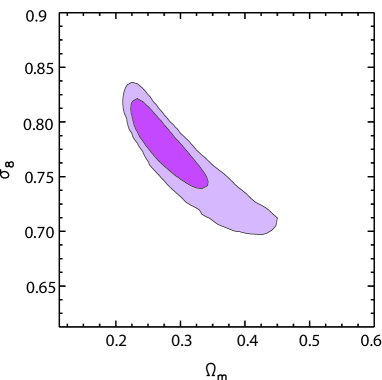
Figure 2: Joint 68.3 and 95.4 per cent confidence constraints on $\Omega_{m}$ and $\sigma_{8}$ for a $\Lambda$CDM model from MACS, BCS, and REFLEX combination using standard priors (as described in the text).

Our previous constraints are in good agreement with recent, independent results from the CMB (Spergel et al. 2007) and cosmic shear, as measured in the 100 Square Degree Survey (Benjamin et al. 2007) and CFHTLS Wide field (Fu et al. 2008). Our results are also in good overall agreement with previous findings based on the observed X-ray luminosity and temperature functions of clusters (Eke et al 1998, Donahue & Voit 1999, Henry 2000, Borgani et al. 2001, Seljak 2002, Allen et al. 2003, Pierpaoli et al. 2003, Schuecker et al. 2003, Henry 2004). Our result on $\Omega_{m}$ is in excellent agreement with current constraints based on cluster $f_{gas}$ data (Allen et al. 2008 and references therein) and the power spectrum of galaxies in the 2dF galaxy redshift survey (Cole et al. 2005) and Sloan Digital Sky Survey (SDSS) (Eisenstein et al. 2005, Tegmark et al. 2006, Percival et al. 2007), as well as the combination of CMB data with a variety of external constraints (Spergel 2007).

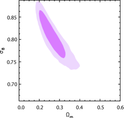
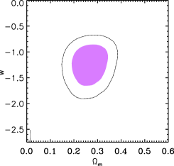
Figure 3: Panel (a). Same as Fig. 2 but for a $w$CDM model. Panel (b). Joint 68.3 and 95.4 per cent confidence constraints on $\Omega_{m}$ and $w$ for a constant-$w$ model using the X-ray luminosity function data and standard priors (as described in the text).

In Fig. 3a, we set constraints for the $w$CDM model, and we plot the joint constraints on $\Omega_{m}$ and $\sigma_{8}$ from the luminosity function data using our standard priors, while Fig. 3b displays constraints on $\Omega_{m}$ and $w$ obtained independently from the XLF data. The marginalized results from the X-ray luminosity function data are $\Omega_{m}=0.27^{+0.07}_{-0.06}$, $\sigma_{8}=0.81^{+0.05}_{-0.06}$ and $w=-1.3^{+0.3}_{-0.4}$, while in M08 they are again less tight $\Omega_{m}=0.24^{+0.15}_{-0.07}$, $\sigma_{8}=0.85^{+0.13}_{-0.20}$ and $w=-1.4^{+0.4}_{-0.7}$. Our new XLF results are consistent with the cosmological-constant model ($w=-1$).

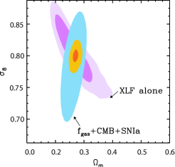
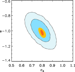
Figure 4: Joint 68.3 and 95.4 per cent confidence constraints on $\Omega_{m}$ and $\sigma_{8}$ (left panel) and $\sigma_{8}$ and $w$ (right panel) obtained from a combined $f_{gas}$+CMB+SNIa analysis (blue) and the improved constraints obtained by combining these data with the XLF (gold). No priors on $h$, $\Omega_{b}h^{2}$ or $n_{s}$ are imposed in either analysis. In the left panel, the results from the XLF alone using standard priors are shown (purple) in order to illustrate the degeneracy breaking. Note that in the left panel we plotted just the inner confidence contours in the $f_{gas}$+CMB+SNIa analysis, in order to have a more readable plot.

An improvement on the previous results can be obtained by adding to the XLF analysis the $f_{gas}$+CMB+SNIa data set. The $f_{gas}$+CMB+SNIa combination already provides tight constraints on $\Omega_{m}$, $h$, $\Omega_{b}h^{2}$ and $n_{s}$ (hence no priors on these parameters are used in either combined analysis), but the degeneracy between $w$ and $\sigma_{8}$ (right panel of Fig. 4) limits the precision of the dark energy results. The addition of the XLF data breaks the degeneracy in the $\Omega_{m}$-$\sigma_{8}$ plane (left panel), resulting in tighter constraints on $\Omega_{m}$, $\sigma_{8}$ and $w$. The degeneracy breaking power of other combinations of data with the CMB is discussed by Spergel et al. (2007). The resulting constraint are $\Omega_{m}=0.269\pm 0.012$, $\sigma_{8}=0.81{\pm 0.021}$ and $w=-1.02{\pm 0.04}$, to be compared with M08 $\Omega_{m}=0.269{\pm 0.016}$, $\sigma_{8}=0.82{\pm 0.03}$ and $w=-1.02{\pm 0.06}$. The previous constraints are in agreement within the errors with Vikhlinin et al. (2009b) constraints, namely $\Omega_{m}=0.255\pm 0.043$, $\sigma_{8}=0.786{\pm 0.011}$ and $w=-0.991{\pm 0.045}$.

It is important to note that the tight constraints obtained by M08 when combining XLF analysis with the $f_{gas}$+CMB+SNIa data set are primarily due to the tightness of the constraints obtained from $f_{gas}$+CMB+SNIa data itself and not to the precision of the XLF analysis of M08, as shown by comparing our results for $\Omega_{m}$, $\sigma_{8}$, $w$ obtained by the XLF analysis with those of M08. In our model the improvement in the mass function model and the L-M relationship gives rise to tight constraints even when using only the XLF function.

In order to understand why the results of our analysis are different from those of M08, we have to stress a key point. The M08 paper, as well as several others papers in the literature, used two different data sets: REFLEX, BCS, and MACS to constrain cosmological parameters and another external data set to constrain the luminosity–mass relation (RB02 data set), which in M08 is a power-law with three free parameters, without explicitly accounting for selection bias. Consequently, it was necessary to restrict that external data set (RB02) to low redshifts and high fluxes in order to minimize the effects of selection bias, making it impossible to test for departures from self-similar evolution in the scaling relation. In order to have a “self-consistent” analysis, it is necessary that a single likelihood function be applied to the full data set which encompasses the entire theoretical model (cosmology + scaling relations) so as to ensure that the covariance among all the model parameters is fully captured and that the effects of the mass function and selection biases are properly accounted for throughout. This kind of analysis was performed for the first time by Vikhlinin et al. (2009a,b), who used the same cluster sample to constrain the scaling relations, thus obtaining tighter constraints.

In the analysis of the present paper, the L–M relation is a physically motivated relation (not a power-law with free parameters) which does not require fits to data, as in M08. Since we do not need the double analysis of M08 and previous papers, the first to get the L–M fitting parameters from RB02 data, and the second to obtain the cosmological constraints using BCS, REFLEX and MACS, we bypass the quoted drawback in the M08 analysis.

It is interesting to note that a month after the present paper was submitted, two papers, Mantz et al. (2009a,b), appeared in arXiv showing that the key point that I previously stressed, namely generalizing M08 to allow the quoted simultaneous and self-consistent fit and using T08 mass function (instead of that in Jenkins et al. 2001) result in cosmological constraints that are a factor 2-3 better than those in M08, based on the same flux-limited sample of clusters. In the present paper, we have also checked that using the same L–M relation used in M08, we reobtain the same set of constraints derived by M08 .

Another point to stress concerns the use of our non-self similar L–M relation for clusters of luminosity $L>3\times 10^{44}$ erg/s in the 0.1–2.4 keV band. Since the clusters included in the M08 sample are high X-ray luminosity (above $3\times 10^{44}$ erg/s), one could think that the changes in the L–M relation of the present paper, with respect to the classical self-similar model, will not produce significant changes in constraints on the cosmological parameters. Even if major differences between the L–M model of the present paper and the self–similar model are observed at gas temperatures below 3 ${\rm keV}$, we stress that the present L–M relation depends on the M–T and L–T relationships, and especially the second one (based on the Modified Punctuated Equilibrium Model (MPEM)) never behaves in a self-similar way as shown in Del Popolo et al. (2005) (even at gas temperatures higher than 10 keV). Moreover, as previously reported, the improvement in the constraints is strictly connected to the fact that we bypass the quoted drawback in the M08 analysis by means of our L–M relation not depending on parameters that must be fixed using external data.

In order to obtain tighter and tighter constraints one needs to try to reduce to the minimum the systematic uncertainties in the analysis. Much progress is expected over the coming years in refining the ranges of these allowances, both observationally and through improved simulations. A reduction in the size of the required systematic allowances will tighten the cosmological constraints. Improved numerical simulations of large samples of massive clusters, including a more complete treatment of star formation and feedback physics that reproduces both the observed optical galaxy luminosity function and cluster X-ray properties, will be of major importance. Further deep X-ray and optical observations of nearby clusters will provide better constraints on the viscosity of the cluster gas. Improved optical/near infrared observations of clusters should pin down the stellar mass fraction in galaxy clusters and its evolution. Ground and space-based gravitational lensing studies will provide important, independent constraints on the mass distributions in clusters; a large program using the Subaru telescope and Hubble Space Telescope is underway, as is similar work by other groups (e.g. Hoekstra 2007).

In the near future, continuing programs of Chandra and XMM-Newton observations of known, X-ray luminous clusters should allow important progress to be made, both by expanding the $f_{gas}$ sample (e.g. Chandra snapshot observations of the entire MACS sample; Ebeling et al. 2001, 2007) and through deeper observations of the current target list. A new, large area X-ray survey such as that proposed by the Spectrum-RG/eROSITA project could make a substantial contribution, finding hundreds of suitable systems at high redshifts.

Looking a decade ahead, the International X-ray Observatory (IXO), result of the merging of NASA’s Constellation-X and ESA/JAXA’s XEUS mission concepts, will offer the possibility to carry out precise studies of dark energy using the $f_{gas}$ technique.

4 Conclusions

In the present paper, we showed how to improve the constraints on $\Omega_{m}$, $\sigma_{8}$, and the dark-energy equation-of-state parameter, $w$, from measurements of the X-ray luminosity function of galaxy clusters, as performed by M08. Improving the mass function by means of Del Popolo (2006a, b) model, which was shown to be in good agreement with T08 and using the L–M relationship obtained in Del Popolo (2002) and Del Popolo et al. (2005), we showed that the XLF alone can give tight constraints on the cosmological parameters. Using the same methods and priors of M08, we find, for a $\Lambda$CDM universe, $\Omega_{m}=0.28^{+0.05}_{-0.04}$ and $\sigma_{8}=0.78^{+0.04}_{-0.05}$ and similarly in the case of a $w$CDM model, we find $\Omega_{m}=0.27^{+0.07}_{-0.06}$, $\sigma_{8}=0.81^{+0.05}_{-0.06}$ and $w=-1.3^{+0.3}_{-0.4}$, both tighter than M08 results. Combining the XLF analysis with the $f_{gas}$+CMB+SNIa data set results in the constraint $\Omega_{m}=0.269\pm 0.012$, $\sigma_{8}=0.81\pm 0.021$ and $w=-1.02\pm 0.04$, in agreement with the most recent determination of the quoted parameters (Allen et al. 2008; Vikhlinin et al. 2009b; Percival et al. 2009). Our findings, consistent with $w=-1$ lends additional support to the cosmological-constant model.

- (1) Allen S. W., Schmidt R. W., Fabian A. C., Ebeling H., 2003, MNRAS, 342, 287
- (2) Allen et al. 2008, MNRAS 383, Issue 3, 879
- (3) Allen, S. W., & Fabian, A. 1998, MNRAS, 297, L57
- (4) Bahcall, N. A. & Fan, X. 1998, ApJ, 504, 1
- (5) Bahcall,N. A., Fan, X., & Cen, R. 1997, ApJ, 485, L53
- (6) Bardeen J.M., Bond, J. R., Kaiser, N., Szalay, A. S. 1986, ApJ 304, 15
- (7) Benjamin, J. et al., 2007, MNRAS, 381, 702
- (8) Bialek, J. J., Evrard, A. E., & Mohr J. J. 2001, ApJ, 555, 597
- (9) Blanchard, A., & Bartlett, J.G. 1998,A&A, 332, L49
- (10) Blanchard, A., Bartlett, J. G., & Sadat, R. 1998, preprint (astro-ph/9809182)
- (11) Böhringer H. et al., 2004, A&A, 425, 367
- (12) Borgani, S. et al., 2001, ApJ, 561, 13
- (13) Bower, R. G., Castander, F. J., Couch, W., Ellis, R. S., & Böhringer, H. 1997, MNRAS, 291, 353
- (14) Bryan,G. L., & Norman,M. L. 1998,ApJ, 495, 80
- (15) Burenin, R. A., Vikhlinin, A., Hornstrup, A., Ebeling, H., Quintana, H., & Mescheryakov, A. 2007, ApJS, 172, 561,
- (16) Cavaliere, A., Menci, N., & Tozzi, P. 1997, ApJ, 484, L21 (CMT97)
- (17) . 1998, ApJ, 501, 493 (CMT98)
- (18) . 1999, MNRAS, 308, 599 (CMT99)
- (19) Cash, A., 1979, ApJ 228, 939
- (20) Cole, S., et al., 2005, MNRAS, 362, 505
- (21) David L.P., Slyz A., Jones C., Forman W., Vrtilek S.D., 1993, ApJ, 412, 479
- (22) Del Popolo A., 2002, MNRAS 336, 81
- (23) Del Popolo A., 2003, ApJ 599, 723
- (24) Del Popolo A., Hiotelis S., Peńarrubia G., 2005, ApJ 628, 76
- (25) Del Popolo, A., 2006a, ApJ 637, 12
- (26) Del Popolo, A., 2006b, AJ 131, 2367
- (27) Donahue,M., & Voit, G.M. 1999,ApJ, 523, L137
- (28) Dunkley, J. et al., 2008, arXiv:0811.4280
- (29) Ebeling H., Edge A. C., Allen S.W., Crawford C. S., Fabian A. C., Huchra J. P., 2000, MNRAS, 318, 333
- (30) Ebeling H., Edge A. C., Bohringer H., Allen S. W., Crawford C. S., Fabian A. C., Voges W., Huchra J. P., 1998,
- (31) Ebeling H., Edge A. C., Henry J. P., 2001, ApJ, 553, 668
- (32) Ebeling H., Barrett E., Donovan D., Ma C. J., Edge A. C., van Speybroeck L., 2007, ApJL, 661, L33
- (33) Edge, A. C., & Stewart, G. C. 1991, MNRAS, 252, 414
- (34) Eke, V. R. et al., 1998, MNRAS, 298, 1145
- (35) Eke, V. R., Cole, S., & Frenk, C. S. 1996, MNRAS, 282, 263
- (36) Eisenstein D. J. et al., 2005, ApJ, 633, 560
- (37) Finoguenov, A., Reiprich, T. H., & Böhringer, H. 2001, A&A, 368, 749
- (38) Freedman W. L. et al., 2001, ApJ, 553, 47
- (39) Fu, L. et al., 2008, A&A, 479, 9
- (40) Gao L., Navarro J. F., Cole S., Frenk C., White S. D. M., Springel V., Jenkins A., Neto A. F., 2007, MNRAS, submitted, arXiv:astro-ph/0711.0746
- (41) Governato, F., Babul, A., Quinn, T., Tozzi, P., Baugh, C., Katz, N., & Lake,G. 1999,MNRAS, 307, 949
- (42) Gregory P. C., & Loredo T., 1992, ApJ 398, 146
- (43) Henry J. P., 2000, ApJ, 534, 565
- (44) Henry J. P., 2004, ApJ, 609, 603
- (45) Henry, J. P. & Arnaud, K. A., 1991, ApJ, 372, 410
- (46) Horner D.J., Mushotzky R.F., Scharf C.A., 1999, ApJ, 520, 78
- (47) Hoekstra H., 2007, MNRAS 379, 317
- (48) Hu W., Kravtsov A. V., 2003, ApJ, 584, 702
- (49) Jenkins A., Frenk C. S., White S. D. M., Colberg J. M., Cole S., Evrard A. E., Couchman H. M. P., Yoshida N., 2001, MNRAS 321, 372
- (50) Jeltema, T. E., Hallman, E. J., Burns, J. O., & Motl, P. M. 2007, ApJ, in press, (ArXiv:0708.1518, 708
- (51) Kaiser, N. 1986, MNRAS, 222, 323
- (52) Kaiser, N. 1991, ApJ, 383, 104
- (53) Kirkman D., Tytler D., Suzuki N., O Meara J. M., Lubin D., 2003, ApJS, 149, 1
- (54) Komatsu, E. et al., 2008, arXiv:0803.0547
- (55) Kravtsov A. V., Vikhlinin A., Nagai D., 2006, ApJ, 650, 128
- (56) Maughan B. J., 2007; ApJ 668, 772
- (57) Mantz et al 2008, MNRAS, 387, 1179 (M08)
- (58) Mantz et al 2009a, arXiv: 0909.3098
- (59) Mantz et al 2009b, arXiv: 0909.3099
- (60) Markevitch M., 1998, ApJ, 503, 77
- (61) Morandi A., Ettori S., Moscardini L., 2007, MNRAS, 379, 518
- (62) Muanwong, O., Thomas, P. A., Kay, S. T., Pearce, F. R., & Couchman, H. M. P. 2001, ApJ, 552, L27
- (63) Nagai, D., Vikhlinin, A., & Kravtsov, A. V. 2007, ApJ, 655, 98
- (64) Navarro, J. F., Frenk, C. S., & White, S. D. M. 1995, MNRAS, 275, 720
- (65) Nevalainen, J., Markevitch, M., & Forman, W. 2000, ApJ, 532, 694
- (66) Percival W. J. et al., 2007, ApJ, 657, 51
- (67) Percival W. J. et al., 2009, astro-ph.CO/0907.1660
- (68) Pierpaoli E., Scott D., White M., 2001, MNRAS, 325, 77
- (69) Pierpaoli E., Borgani S., Scott D., White M., 2003, MNRAS, 342, 163
- (70) Ponman, T. J., Cannon, D. B., & Navarro, J. F. 1999, Nature, 397, 135
- (71) Press W., & Schechter P., 1974, ApJ 187, 425
- (72) Rasia, E., et al. 2006, MNRAS, 369, 2013
- (73) Reed, D., et al. 2003, MNRAS, 346, 565 (R03)
- (74) Reichart, D. E., Nichol, R. C., Castander, F. J., Burke, D. J., Romer, A. K., Holden, B. P., Collins, C. A., & Ulmer, M. P. 1999b, ApJ, 518, 521
- (75) Reiprich, T. H. & Böhringer, H., 2002, ApJ, 567, 716
- (76) Rosati, P., Borgani S., and Norman, C., Ann. Rev. Astron. Astrophys 2002, 40: 539-77
- (77) Sadat,R., Blanchard, A., & Oukbir, J. 1998,A&A, 329, 21
- (78) Schuecker, P. et al., 2003, A&A, 398, 867
- (79) Seljak U., 2002, MNRAS, 337, 769
- (80) Sheth R. K., & Tormen G., 2002, MNRAS 329, 61
- (81) Spergel, D. N. et al., 2007, ApJS, 170, 377
- (82) Tegmark M. et al., 2006, Phys. Rev. D, 74, 123507
- (83) Tinker et al. 2008, ApJ 688, 709
- (84) Tozzi, P., & Norman, C. 2001, ApJ, 546, 63
- (85) Trümper J., 1993, Science, 260, 1769
- (86) Viana, P. T. P., & Liddle, A. R. 1999, MNRAS, 303, 535
- (87) Voit, C.M. 2000, ApJ, 543, 113
- (88) Vikhlinin, A., McNamara, B. R., Forman, W., Jones, C., Quintana, H., & Hornstrup, A. 1998, ApJ 502, 558
- (89) Vikhlinin, A. et al., 2009a, ApJ 692, 1033
- (90) Vikhlinin, A. et al., 2009b, ApJ 692, 1060
- (91) Voevodkin A., Vikhlinin A., 2004, ApJ, 601, 610
- (92) Voit, C.M., & Donahue,M. 1998,ApJ, 500, L111
- (93) Voit, G. M., & Bryan, G. 2001, Nature, 414, 425
- (94) Warren, M. S., Abazajian, K., Holz, D. E., & Teodoro, L. 2006, ApJ, 646, 881
- (95) White S.D.M., Navarro J.F., Evrard A.E., Frenk C.S., 1993, Nature, 366, 429.
- (96) Xu, H., Jing, G., & Wu, X. 2001, ApJ, 553, 78
- (97) Yahagi, H., Nagashima, M., & Yoshii, Y. 2004, ApJ, 605, 709 (YNY04)
- (98) Zhang, Y. Y., Finoguenov A., Böhringer H., Kneib J. P., Smith G. P., Czoske O., Soucail G., 2007, A&A 467, 437