Graph-Constrained Group Testing

Abstract

Non-adaptive group testing involves grouping arbitrary subsets of $n$ items into different pools. Each pool is then tested and defective items are identified. A fundamental question involves minimizing the number of pools required to identify at most $d$ defective items. Motivated by applications in network tomography, sensor networks and infection propagation, a variation of group testing problems on graphs is formulated. Unlike conventional group testing problems, each group here must conform to the constraints imposed by a graph. For instance, items can be associated with vertices and each pool is any set of nodes that must be path connected. In this paper, a test is associated with a random walk. In this context, conventional group testing corresponds to the special case of a complete graph on $n$ vertices.

For interesting classes of graphs a rather surprising result is obtained, namely, that the number of tests required to identify $d$ defective items is substantially similar to what is required in conventional group testing problems, where no such constraints on pooling is imposed. Specifically, if $T(n)$ corresponds to the mixing time of the graph $G$, it is shown that with $m=O(d^{2}T^{2}(n)\log(n/d))$ non-adaptive tests, one can identify the defective items. Consequently, for the Erdős-Rényi random graph $G(n,p)$, as well as expander graphs with constant spectral gap, it follows that $m=O(d^{2}\log^{3}n)$ non-adaptive tests are sufficient to identify $d$ defective items. Next, a specific scenario is considered that arises in network tomography, for which it is shown that $m=O(d^{3}\log^{3}n)$ non-adaptive tests are sufficient to identify $d$ defective items. Noisy counterparts of the graph constrained group testing problem are considered, for which parallel results are developed. We also briefly discuss extensions to compressive sensing on graphs.

I Introduction

In this paper we introduce the graph constrained group testing problem motivated by applications in network tomography, sensor networks and infection propagation. While group testing theory (see  [1, 2] and more recently [3]), and its numerous applications, such as industrial quality assurance [4], DNA library screening [5], software testing [6], and multi-access communications [7], have been systematically explored, the graph constrained group testing problem is new to the best of our knowledge.

Group testing involves identifying at most $d$ defective items out of a set of $n$ items. In non-adaptive group testing, which is the subject of this paper, we are given an $m\times n$ binary matrix, $M$, usually referred to as a test or measurement matrix. Ones on the $j$th row of $M$ indicate which subset of the $n$ items belongs to the $j$th pool. A test is conducted on each pool; a positive outcome indicating that at least one defective item is part of the pool; and a negative test indicating that no defective items are part of the pool. The conventional group testing problem is to design a matrix $M$ with minimum number of rows $m$ that guarantees error free identification of the defective items. While the best known (probabilistic) pooling design requires a test matrix with $m=O(d^{2}\log(n/d))$ rows, and an almost-matching lower bound of $m=\Omega(d^{2}(\log n)/(\log d))$ is known on the number of pools (cf. [2, Chapter 7]), the size of the optimal test still remains open.

Note that in the standard group testing problem the test matrix $M$ can be designed arbitrarily. In this paper we consider a generalization of the group testing problem to the case where the matrix $M$ must conform to constraints imposed by a graph $G=(V,E)$. In general, as we will describe shortly, such problems naturally arise in several applications such as network tomography [8, 9], sensor networks [10], and infection propagation [11]. While the graph constrained group testing problem has been alluded to in these applications, the problem of test design or the characterization of the minimum number of tests, to the best of our knowledge, has not been addressed before. In this light our paper is the first to formalize the graph constrained group testing problem. In our graph group testing problem the $n$ items are either vertices or links (edges) of the graph; at most $d$ of them are defective. The task is to identify the defective vertices or edges. The test matrix $M$ is constrained as follows: for items associated with vertices each row must correspond to a subset of vertices that are connected by a path on the graph; similarly, for items associated with links each row must correspond to links that form a path on $G$. The task is to design an $m\times n$ binary test matrix with minimum number of rows $m$ that guarantees error free identification of the defective items.

We will next describe several applications, which illustrate the graph constrained group testing problem.

I-A Network Tomography & Compressed Sensing over Graphs

For a given network, identification of congested links from end-to-end path measurements is one of the key problems in network tomography [9], [8]. In many settings of today’s IP networks, there is one or a few links along the path which cause the packet losses in the path. Finding the locations of such congested links is sufficient for most of the practical applications.

This problem can be understood as a graph-constrained group testing as follows. We model the network as a graph $G=(V,E)$ where the set $V$ denotes the network routers/hosts and the set $E$ denotes the communication links (see Fig. 1). Suppose, we have a monitoring system that consists of one or more end hosts (so called vantage points) that can send and receive packets. Each vantage point sends packets through the network by assigning the routes and the end hosts.

All measurement results (i.e., whether each packet has reached its destination) will be reported to a central server whose responsibility is to identify the congested links. Since the network is given, not any route is a valid one. A vantage point can only assign those routes which form a path in the graph $G$. The question of interest is to determine the number of measurements that is needed in order to identify the congested links in a given network.

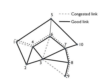
Figure 1: The route $1\rightarrow 4\rightarrow 6\rightarrow 7\rightarrow 8\rightarrow 9$ is valid while $2\rightarrow 6\rightarrow 5$ is not.

We primarily deal with Boolean operations on binary valued variables in this paper, namely, link states are binary valued and the measurements are boolean operations on the link states. Nevertheless, the techniques described here can be extended to include non-boolean operations and non-binary variables as well. Specifically, suppose there are a sparse set of links that take on non-zero values. These non-zero values could correspond to packet delays, and packet loss probabilities along each link. Measurements along each path provides aggregate delay or aggregate loss along the path. The set of paths generated by $m$ random walks forms a $m\times|E|$ routing matrix $M$. For an appropriate choice of $m$ and graphs studied in this paper, it turns out (see [12]) that such routing matrices belongs to the class of so called expander matrices. These expander type properties in turn obey a suitable type of restricted-isometry-property (1-RIP) [13]. Such properties in turn are sufficient for recovering sparse vectors using $\ell_{1}$ optimization techniques. Consequently, the results of this paper have implications for compressed sensing on graphs.

I-B Sensor Networks

The network tomography problem is further compounded in wireless sensor networks (WSN). As described in [10] the routing topology in WSN is constantly changing due to the inherent ad-hoc nature of the communication protocols. The sensor network is static with a given graph topology such as a geometric random graph. Sensor networks can be monitored passively or actively. In passive monitoring, at any instant, sensor nodes form a tree to route packets to the sink. The routing tree constantly changes unpredictably but must be consistent with the underlying network connectivity. A test is considered positive if the arrival time is significantly large, which indicates that there is at least one defective sensor node or a congested link. The goal is to identify defective links or sensor nodes based on packet arrival times at the sink. In active monitoring network nodes continuously calculate some high level, summarized information such as the average or maximum energy level among all nodes in the network. When the high level information indicates congested links, a low level and more energy consuming procedure is used to accurately locate the trouble spots.

I-C Infection Propagation

Suppose that we have a large population where only a small number of people are infected by a certain viral sickness (e.g., a flu epidemic). The task is to identify the set of infected individuals by sending agents among them. Each agent contacts a pre-determined or randomly chosen set of people. Once an agent has made contact with an infected person, there is a chance that he gets infected, too. By the end of the testing procedure, all agents are gathered and tested for the disease. While this problem has been described in [11], the analysis ignores the inherent graph constraints that need to be further imposed. It is realistic to assume that, once an agent has contacted a person, the next contact will be with someone in close proximity of that person. Therefore, in this model we are given a random geometric graph that indicates which set of contacts can be made by an agent (see Fig. 2). Now, the question is to determine the number of agents that is needed in order to identify the set of infected people.

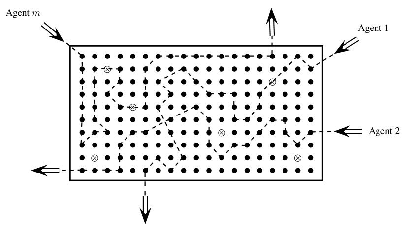
Figure 2: Collective sampling using agents. The $\otimes$ symbols represent infected people whereas the healthy population is indicated by $\bullet$ symbols. The dashed lines show the group of people contacted by each agent [11].

These applications present different cases where graph constrained group testing can arise. However, there are important distinctions. In the wired network tomography scenario the links are the items and each row of the matrix $M$ is associated with a route between any two vantage points. A test is positive if a path is congested, namely, if it contains at least one congested link. Note that in this case since the routing table is assumed to be static, the route between any two vantage points is fixed. Consequently, the matrix $M$ is deterministic and the problem reduces to determining whether or not the matrix $M$ satisfies identifiability.

Our problem is closer in spirit to the wireless sensor network scenario. In the passive case the links are the items and each row of the matrix $M$ is associated with a route between a sensor node and the sink. A test is positive if a path is congested, namely, if it contains at least one congested link. Note that in this case since the routing table is constantly changing, the route between a sensor node and the sink is constantly changing as well. Nevertheless the set of possible routes must be drawn from the underlying connectivity graph. Consequently, the matrix $M$ can be assumed to be random and the problem is to determine how many different tests are required to identify the congested links. Note that, in contrast to the wired scenario, tests conducted between the same sensor node and sink yields new information here. A similar situation arises in the active monitoring case as well. Here one could randomly query along different routes to determine whether or not a path is congested. These tests can be collated to identify congested links. Note that in the active case the test matrix $M$ is amenable to design in that one could selectively choose certain paths over others by considering weighted graphs.

Motivated by the WSN scenario we describe pool designs based on random walks on graphs. As is well known a random walk is the state evolution on a finite reversible Markov chain. Each row of the binary test matrix is derived from the evolution of the random walk, namely, the ones on the $j$th row of $M$ correspond to the vertices visited by the $j$th walk. This is close to the WSN scenario because as in the WSN scenario the path between two given nodes changes randomly. We develop several results in this context.

First, we consider random walks that start either at a random node or an arbitrary node but terminate after some appropriately chosen number of steps $t$. By optimizing the length of the walk we arrive at an interesting result for important classes of graphs. Specifically we show that the number of tests required to identify $d$ defective items is substantially similar to that required in conventional group testing problems, except the fact that an extra term appears which captures the topology of the underlying graph. The best known result for the number of tests required when no graphical constraints are imposed scales as $O(d^{2}\log(n/d))$. For the graph constrained case we show that with $m=O(d^{2}T^{2}(n)\log(n/d))$ non-adaptive tests one can identify the defective items, where $T(n)$ corresponds to the mixing time of the underlying graph $G$. Consequently, for the Erdős-Rényi random graph $G(n,p)$ with $p=\Omega((\log^{2}n)/n)$, as well as expander graphs with constant spectral gap, it follows that $m=O(d^{2}\log^{3}n)$ non-adaptive tests are sufficient to identify $d$ defective items. In particular, for a complete graph where no pooling constraint is imposed, we have $T(n)=1$, and therefore, our result subsumes the well-known result for the conventional group testing problem.

Next we consider unbounded-length random walks that originate at a source node and terminate at a sink node. Both the source node and the sink node can either be arbitrary or be chosen uniformly at random. This directly corresponds to the network tomography problem that arises in the WSN context. This is because the source nodes can be viewed as sensor nodes, while the sink node maybe viewed as the fusion center, where data is aggregated. At any instant, we can assume that a random tree originating at the sensor nodes and terminating at the sink is realized. While this random tree does not have cycles, there exist close connections between random walks and randomly generated trees. Indeed, it is well known that the so called loop-erased random walks, obtained by systematically erasing loops in random walks, to obtain spanning trees, is a method for sampling spanning trees from a uniform distribution [14]. In this scenario, we show that $m=O(d^{3}\log^{3}n)$ non-adaptive tests are sufficient to identify $d$ defective items. By considering complete graphs we also establish that the cubic dependence on $d$ in this result cannot be improved.

We will also consider noisy counterparts of the graph constrained group testing problem, where the outcome of each measurement may be independently corrupted (flipped) with probability $0\leq q<1/2$. We develop parallel results for these cases. In addition to a setting with noisy measurement outcomes, these results can be used in a so called dilution model (as observed in [3, 11]). In this model, each item can be diluted in each test with some a priori known probability. In a network setting, this would correspond to the case where a test on a path with a congested link can turn out to be negative with some probability. We show that similar scaling results holds for this case as well.

Other group testing problems on graphs: Several variations of classical group testing have been studied in the literature that possess a graph theoretic nature. A notable example is the problem of learning hidden sparse subgraphs (or more generally, hypergraphs), defined as follows (cf. [15]): Assume that, for a given graph, a small number of the edges are marked as defective. The problem is to use a small number of measurements of the following type to identify the set of defective edges: Each measurement specifies a subset of vertices, and the outcome would be positive iff the graph induced on the subset contains a defective edge. Another variation concerns group testing with constraints defined by a rooted tree. Namely, the set of items corresponds to the leaves of a given rooted tree, and each test is restricted to pool all the leaves that descend from a specified node in the tree (see [2, Chapter 12]). To the best of our knowledge, our work is the first variation to consider the natural restriction of the pools with respect to the paths on a given graph.

The rest of this paper is organized as follows. In Section II, we introduce our notation and mention some basic facts related to group testing and random walks on graphs. Section III formally describes the problem that we consider and states our main results. In Section IV we prove the main results, and finally, in Section V show instantiations of the result to the important cases of graph-constrained group testing on regular expander graphs and random graphs in the Erdős-Rényi model.

II Definitions and Notation

In this section we introduce some tools, definition and notations which are used throughout the paper.

Definition 1.

For two given boolean vectors $S$ and $T$ of the same length we denote their element-wise logical $\mathsf{or}$ by $S\vee T$. More generally, we will use $\bigvee_{i=1}^{d}S_{i}$ to denote the element-wise $\mathsf{or}$ of $d$ boolean vectors $S_{1},\ldots,S_{d}$. The logical subtraction of two boolean vectors $S=(s_{1},\ldots,s_{n})$ and $T=(t_{1},\ldots,t_{n})$, denoted by $S\setminus T$, is defined as a boolean vector which has a $1$ at position $i$ if and only if $s_{i}=1$ and $t_{i}=0$. We also use $|S|$ to show the number of $1$’s in (i.e., the Hamming weight of) a vector $S$.

We often find it convenient to think of boolean vectors as characteristic vectors of sets. That is, $x\in\{0,1\}^{n}$ would correspond to a set $X\subseteq[n]$ (where $[n]:=\{1,\ldots,n\}$) such that $i\in X$ iff the entry at the $i$th position of $x$ is $1$. In this sense, the above definition extends the set-theoretic notions of union, subtraction, and cardinality to boolean vectors.

Matrices that are suitable for the purpose of group testing are known as disjunct matrices. The formal definition is as follows.

Definition 2.

An $m\times n$ boolean matrix $M$ is called $d$-disjunct, if, for every column $S_{0}$ and every choice of $d$ columns $S_{1},\ldots,S_{d}$ of $M$ (different from $S_{0}$), there is at least one row at which the entry corresponding to $S_{0}$ is $1$ and those corresponding to $S_{1},\ldots,S_{d}$ are all zeros. More generally, for an integer $e\geq 0$, the matrix is called $(d,e)$-disjunct if for every choice of the columns $S_{i}$ as above, they satisfy

$$|S_{0}\setminus\bigvee_{i=1}^{d}S_{i}|>e.$$

A $(d,0)$-disjunct matrix is said to be $d$-disjunct.

A classical observation in group testing theory states that disjunct matrices can be used in non-adaptive group testing schemes to distinguish sparse boolean vectors (cf. [2]). More precisely, suppose that a $d$-disjunct matrix $M$ with $n$ columns is used as the measurement matrix; i.e., we assume that the rows of $M$ are the characteristic vectors of the pools defined by the scheme. Then, the test outcomes obtained by applying the scheme on two distinct $d$-sparse vectors of length $n$ must differ in at least one position. More generally, if $M$ is taken to be $(d,e)$-disjunct, the test outcomes must differ in at least $e+1$ positions. Thus, the more general notion of $(d,e)$-disjunct matrices is useful for various “noisy” settings, where we are allowed to have a few false outcomes (in particular, up to $\lfloor(e-1)/2\rfloor$ incorrect measurement outcomes can be tolerated by $(d,e)$-disjunct matrices without causing any confusion).

For our application, sparse vectors (that are to be distinguished) correspond to boolean vectors encoding the set of defective vertices (or edges) in a given undirected graph. The encoding is such that the coordinate positions are indexed by the set of vertices (edges) of the graph and a position contains $1$ iff it corresponds to a defective vertex (edge). Moreover, we aim to construct disjunct matrices that are also constrained to be consistent with the underlying graph.

Definition 3.

Let $G=(V,E)$ be an undirected graph, and $A$ and $B$ be boolean matrices with $|V|$ and $|E|$ columns, respectively. The columns of $A$ are indexed by the elements of $V$ and the columns of $B$ are indexed by the elements of $E$. Then,

• The matrix $A$ is said to be vertex-consistent with $G$ if each row of $A$, seen as the characteristic vector of a subset of $V$, exactly represents the set of vertices visited by some walk on $G$.

• The matrix $B$ is said to be edge-consistent with $G$ if each row of $B$, seen as the characteristic vector of a subset of $E$, exactly corresponds to the set of edges traversed by a walk on $G$.

Note that the choice of the walk corresponding to each row of $A$ or $B$ need not be unique. Moreover, a walk may visit a vertex (or edge) more than once.

Definition 4.

An undirected graph $G=(V,E)$ is called $(D,c)$-uniform, for some $c\geq 1$, if the degree of each vertex $v\in V$ (denoted by $\deg(v)$) is between $D$ and $cD$.

Definition 5.

The point-wise distance of two probability distributions $\mu,\mu^{\prime}$ on a finite space $\Omega$ is defined as

$$\|\mu-\mu^{\prime}\|_{\infty}:=\max_{i\in\Omega}|\mu(i)-\mu^{\prime}(i)|,$$

where $\mu(i)$ (resp., $\mu^{\prime}(i)$) denotes the probability assigned by $\mu$ (resp., $\mu^{\prime}$) to the outcome $i\in\Omega$. We say that the two distributions are $\delta$-close if their point-wise distance is at most $\delta$.

For notions such as random walks, stationary distribution and mixing time we refer to many text books on probability theory, Markov chains, and randomized algorithms. In particular for an accessible treatment of the basic notions, see [16, Chapter 6] or [17, Chapter 7]. The particular variation of the mixing time that we will use in this work is defined with respect to the point-wise distance as follows.

Definition 6.

Let $G=(V,E)$ with $|V|=n$ be a $(D,c)$-uniform graph and denote by $\mu$ its stationary distribution. For $v\in V$ and an integer $\tau$, denote by $\mu^{\tau}_{v}$ the distribution that a random walk of length $\tau$ starting at $v$ ends up at. Then, the $\delta$-mixing time of $G$ (with respect to the $\ell_{\infty}$ norm) is the smallest integer $t$ such that $\|\mu^{\tau}_{v}-\mu\|_{\infty}\leq\delta$, for $\forall\tau\geq t$ and $\forall v\in V$. For concreteness, we define the quantity $T(n)$ as the $\delta$-mixing time of $G$ for $\delta:=(1/2cn)^{2}$.

Throughout this work, the constraint graphs are considered to be $(D,c)$-uniform, for an appropriate choice of $D$ and some (typically constant) parameter $c$. When $c=1$, the graph is $D$-regular.

For a graph to have a small mixing time, a random walk starting from any vertex must quickly induce a uniform distribution on the vertex set of the graph. Intuitively this happens if the graph has no “bottle necks” at which the walk can be “trapped”, or in other words, if the graph is “highly connected”. The standard notion of conductance, as defined below, quantifies the connectivity of a graph.

Definition 7.

Let $G=(V,E)$ be a graph on $n$ vertices. For every $S\subseteq V$, define $\Delta(S):=\sum_{v\in S}\deg(v)$, $\bar{S}:=V\setminus S$, and denote by $E(S,\bar{S})$ the number of edges crossing the cut defined by $S$ and its complement. Then the conductance of $G$ is defined by the quantity

$$\Phi(G):=\min_{S\subseteq V\colon\Delta(S)\leq|E|}\frac{E(S,\bar{S})}{\Delta(S)}.$$

We also formally define two important classes of graphs, for which we will specialize our results.

Definition 8.

Take a complete graph on $n$ vertices, and remove edges independently with probability $1-p$. The resulting graph is called the Erdős-Rényi random graph, and denoted by $G(n,p)$.

Definition 9.

For a graph $G=(V,E)$ with $|V|=n$, the (edge) expansion of $G$ is defined as

$$h(G)=\min_{S\subseteq V\colon 0<|S|\leq\frac{n}{2}}\frac{E(S,\bar{S})}{|S|}.$$

A family $\mathcal{G}$ of $D$-regular graphs is called an (edge) expander family if there exists a constant $\sigma>0$ such that $h(G)\geq\sigma$ for each $G\in\mathcal{G}$. In particular each $G\in\mathcal{G}$ is called an expander graph.

For a general study of Erdős-Rényi random graphs and their properties we refer to the fascinating book of Bollobás [18]. For the terminology on expander graphs, we refer the reader to the excellent survey by Hoory, Linial and Wigderson [19].

Definition 10.

Consider a particular random walk $W:=(v_{0},v_{1},\ldots,v_{t})$ of length $t$ on a graph $G=(V,E)$, where the random variables $v_{i}\in V$ denote the vertices visited by the walk, and form a Markov chain. We distinguish the following quantities related to the walk $W$:

• For a vertex $v\in V$ (resp., edge $e\in E$), denote by $\pi_{v}$ (resp., $\pi_{e}$) the probability that $W$ passes $v$ (resp., $e$).

• For a vertex $v\in V$ (resp., edge $e\in E$) and subset $A\subseteq V$, $v\notin A$ (resp., $B\subseteq E$, $e\notin B$), denote by $\pi_{v,A}$ (resp., $\pi_{e,B}$) the probability that $W$ passes $v$ but none of the vertices in $A$ (resp., passes $e$ but none of the edges in $B$).

Note that these quantities are determined by not only $v,e,A,B$ (indicated as subscripts) but they also depend on the choice of the underlying graph, the distribution of the initial vertex $v_{0}$ and length of the walk $t$. However, we find it convenient to keep the latter parameters implicit when their choice is clear from the context.

In the previous definition, the length of the random walk was taken as a fixed parameter $t$. Another type of random walks that we consider in this work have their end points as a parameter and do not have an a priori fixed length. In the following, we define similar probabilities related to the latter type of random walks.

Definition 11.

Consider a particular random walk $W:=(v_{0},v_{1},\ldots,u)$ on a graph $G=(V,E)$ that continues until it reaches a fixed vertex $u\in V$. We distinguish the following quantities related to $W$: For a vertex $v\in V$ (resp., edge $e\in E$) and subset $A\subseteq V$, $v\notin A$ (resp., $B\subseteq E$, $e\notin B$), denote by $\pi^{(u)}_{v,A}$ (resp., $\pi^{(u)}_{e,B}$) the probability that $W$ passes $v$ but none of the vertices in $A$ (resp., passes $e$ but none of the edges in $B$).

Again these quantities depend on the choice of $G$ and the distribution of $v_{0}$ that we will keep implicit.

III Problem setting and Main Results

Problem Statement. Consider a given graph $G=(V,E)$ in which at most $d$ vertices (resp., edges) are defective. The goal is to characterize the set of defective items using a number of measurements that is as small as possible, where each measurement determines whether the set of vertices (resp., edges) observed along a path on the graph has a non-empty intersection with the defective set. We call the problem of finding defective vertices vertex group testing and that of finding defective edges edge group testing.

As mentioned earlier, not all sets of vertices can be grouped together, and only those that share a path on the underlying graph $G$ can participate in a pool (see Fig. 3).

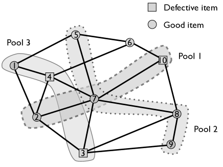
Figure 3: The result of pool 1 is positive since it contains a defective item, whereas the result of pool 2 is negative since it does not contain a defective item. Pool 3 is not consistent with the graph and thus not allowed since the items are not connected by a path.

In the following, we introduce four random constructions (designs) for both problems. The proposed designs follow the natural idea of determining pools by taking random walks on the graph.

Design 1. Given: a constraint graph $G=(V,E)$ with $r\geq 0$ designated vertices $s_{1},\ldots,s_{r}\in V$, and integer parameters $m$ and $t$. Output: an $m\times|V|$ boolean matrix $M$. Construction: Construct each row of $M$ independently as follows: Let $v\in V$ be any of the designated vertices $s_{i}$, or otherwise a vertex chosen uniformly at random from $V$. Perform a random walk of length $t$ starting from $v$, and let the corresponding row of $M$ be the characteristic vector of the set of vertices visited by the walk.

Design 2. Given: a constraint graph $G=(V,E)$ and integer parameters $m$ and $t$. Output: an $m\times|E|$ boolean matrix $M$. Construction: Construct each row of $M$ independently as follows: Let $v\in V$ be any arbitrary vertex of $G$. Perform a random walk of length $t$ starting from $v$, and let the corresponding row of $M$ be the characteristic vector of the set of edges visited by the walk.

Design 3. Given: a constraint graph $G=(V,E)$ with $r\geq 0$ designated vertices $s_{1},\ldots,s_{r}\in V$, a sink node $u\in V$, and integer parameter $m$. Output: an $m\times|V|$ boolean matrix $M$. Constructions: Construct each row of $M$ independently as follows: Let $v\in V$ be any of the designated vertices $s_{i}$, or otherwise a vertex chosen uniformly at random from $V$. Perform a random walk starting from $v$ until we reach $u$, and let the corresponding row of $M$ be the characteristic vector of the set of vertices visited by the walk.

Design 4. Given: a constraint graph $G=(V,E)$, a sink node $u\in V$, and integer parameter $m$. Output: an $m\times|E|$ boolean matrix $M$. Construction: Construct each row of $M$ independently as follows: Let $v\in V$ be any arbitrary vertex of $G$. Perform a random walk, starting from $v$ until we reach $u$, and let the corresponding row of $M$ be the characteristic vector of the set of edges visited by the walk.

By construction, Designs 1 and 3 (resp., Designs 2 and 4) output boolean matrices that are vertex- (resp., edge-) consistent with the graph $G$. Our main goal is to show that, when the number of rows $m$ is sufficiently large, the output matrices become $d$-disjunct (for a given parameter $d$) with overwhelming probability.

Remark 12.

Designs 1 and 3 in particular provide two choices for constructing the measurement matrix $M$. Namely, the start vertices can be chosen within a fixed set of designated vertices, or, chosen randomly among all vertices of the graph. As we will see later, in theory there is no significant difference between the two schemes. However, for some applications it might be the case that only a small subset of vertices are accessible as the starting points (e.g., in network tomography such a subset can be determined by the vantage points), and this can be modeled by an appropriate choice of the designated vertices in Designs 1 and 3.

TABLE I: The asymptotic values of various parameters in Theorem 13.

Parameter	Value
$D_{0}$	$O(c^{2}dT^{2}(n))$
$m_{1},m_{2}$	$O(c^{4}d^{2}T^{2}(n)\log(n/d))$
$m_{3}$	$O(c^{8}d^{3}T^{4}(n)\log(n/d))$
$m_{4}$	$O(c^{9}d^{3}DT^{4}(n)\log(n/d))$
$t_{1}$	$O(n/(c^{3}dT(n)))$
$t_{2}$	$O(nD/(c^{3}dT(n)))$
$e_{1},e_{2},e_{3},e_{4}$	$\Omega(\eta d\log(n/d)/(1-\eta)^{2})$
$m^{\prime}_{i},i\in[4]$	$O(m_{i}/(1-\eta)^{2})$

The following theorem states the main result of this work, showing that our proposed designs indeed produce disjunct matrices that can be used for the purpose of graph-constrained group testing. We will state both noiseless results (corresponding to $d$-disjunct matrices), and noisy ones (corresponding to $(d,e)$-disjunct ones, where the noise tolerance $e$ depends on a fixed “noise parameter” $\eta\in[0,1)$). The proof of the following theorem is given in Section IV.

Theorem 13.

Let $\eta\geq 0$ be a fixed parameter, and suppose that $G=(V,E)$ is a $(D,c)$-uniform graph on $n$ vertices with $\delta$-mixing time $T(n)$ (where $\delta:=(1/2cn)^{2}$). Then there exist parameters with asymptotic values given in Table I such that, provided that $D\geq D_{0}$,

1. Design 1 with the path length $t:=t_{1}$ and the number of measurements $m:=m_{1}$ outputs a matrix $M$ that is vertex-consistent with $G$. Moreover, once the columns of $M$ corresponding to the designated vertices $s_{1},\ldots,s_{r}$ are removed, the matrix becomes $d$-disjunct with probability $1-o(1)$. More generally, for $m:=m^{\prime}_{1}$ the matrix becomes $(d,e_{1})$-disjunct with probability $1-o(1)$.

2. Design 2 with path length $t:=t_{2}$ and $m:=m_{2}$ measurements outputs a matrix $M$ that is edge-consistent with $G$ and is $d$-disjunct with probability $1-o(1)$. More generally, for $m:=m^{\prime}_{2}$ the matrix becomes $(d,e_{2})$-disjunct with probability $1-o(1)$.

3. Design 3 with the number of measurements $m:=m_{3}$ outputs a matrix $M$ that is vertex-consistent with $G$. Moreover, once the columns of $M$ corresponding to the designated vertices $s_{1},\ldots,s_{r}$ and the sink node $u$ are removed, the matrix becomes $d$-disjunct with probability $1-o(1)$. More generally, for $m:=m^{\prime}_{3}$ the matrix becomes $(d,e_{3})$-disjunct with probability $1-o(1)$.

4. Design 4 with the number of measurements $m:=m_{4}$ outputs a matrix $M$ that is edge-consistent with $G$ and is $d$-disjunct with probability $1-o(1)$. More generally, for $m:=m^{\prime}_{4}$ the matrix becomes $(d,e_{4})$-disjunct with probability $1-o(1)$.

Remark 14.

In Designs 1 and 3, we need to assume that the designated vertices (if any) are not defective, and hence, their corresponding columns can be removed from the matrix $M$. By doing so, we will be able to ensure that the resulting matrix is disjunct. Obviously, such a restriction cannot be avoided since, for example, $M$ might be forced to contain an all-ones column corresponding to one of the designated vertices and thus, fail to be even $1$-disjunct.

Remark 15.

By applying Theorem 13 on the complete graph (using Design 1), we get $O(d^{2}\log(n/d))$ measurements, since in this case, the mixing time is $T(n)=1$ and also $c=1$. Thereby, we recover the trade-off obtained by the probabilistic construction in classical group testing (note that classical group testing corresponds to graph-constrained group testing on the vertices of the complete graph).

We will show in Section V that, for our specific choice of $\delta:=(1/2cn)^{2}$, the $\delta$-mixing time of an Erdős-Rényi random graph $G(n,p)$ is (with overwhelming probability) $T(n)=O(\log n)$. This bound more generally holds for any graph with conductance $\Omega(1)$, and in particular, expander graphs with constant spectral gap. Thus we have the following result (with a summary of the achieved parameters given in Table II).

Theorem 16.

There is an integer $D_{0}=\Omega(d\log^{2}n)$ such that for every $D\geq D_{0}$ the following holds: Suppose that the graph $G$ is either

1. A $D$-regular expander graph with normalized second largest eigenvalue (in absolute value) $\lambda$ that is bounded away from $1$; i.e., $\lambda=1-\Omega(1)$, or,

2. An Erdős-Rényi random graph $G(n,D/n)$.

Then for every $\eta\in[0,1)$, with probability $1-o(1)$ Designs 1, 2, 3, and 4 output $(d,e)$-disjunct matrices (not considering the columns corresponding to the designated vertices and the sink in Designs 1 and 3), for some $e=\Omega(\eta d\log n)$, using respectively $m_{1},m_{2},m_{3},m_{4}$ measurements, where $m_{1},m_{2}=O(d^{2}(\log^{3}n)/(1-\eta)^{2})$, $m_{3}=O(d^{3}(\log^{5}n)/(1-\eta)^{2})$, and $m_{4}=O(d^{3}D(\log^{5}n)/(1-\eta)^{2})$.

TABLE II: The asymptotic values of the bounds achieved by Theorem 16.

Parameter	Value
$D_{0}$	$O(d\log^{2}n)$
$m_{1},m_{2}$	$O(d^{2}(\log^{3}n)/(1-p)^{2})$
$m_{3}$	$O(d^{3}(\log^{5}n)/(1-p)^{2})$
$m_{4}$	$O(d^{3}D(\log^{5}n)/(1-p)^{2})$
$e$	$\Omega(\eta d\log n)$

The fixed-input case. Recall that, as Theorem 13 shows, our proposed designs almost surely produce disjunct matrices using a number of measurements summarized in Table I. Thus, with overwhelming probability, once we fix the resulting matrix, it has the combinatorial property of distinguishing between any two $d$-sparse boolean vectors (each corresponding to a set of up to $d$ defective vertices, not including designated ones, for Designs 1 and 3, or up to $d$ defective edges for Designs 2 and 4) in the worst case. However, the randomized nature of our designs can be used to our benefit to show that, practically, one can get similar results with a number of measurements that is almost by a factor $d$ smaller than what required by Theorem 13. Of course, assuming a substantially lower number of measurements, we should not expect to obtain disjunct matrices, or equivalently, to be able to distinguish between any two sparse vectors in the worst case. However, it can be shown that, for every fixed $d$-sparse vector $x$, the resulting matrix with overwhelming probability will be able to distinguish between $x$ and any other $d$-sparse vector using a lower number of measurements. In particular, with overwhelming probability (over the choice of the measurements), from the measurement outcomes obtained from $x$, it will be possible to uniquely reconstruct $x$. More precisely, it is possible to show the following theorem, as proved in Section IV.

Theorem 17.

Consider the assumptions of Theorem 13, and let $\gamma:=(\log n)/(d\log(n/d))$. Consider any fixed set of up to $d$ vertices $S\subseteq V$ such that $|S|\leq d$ and $S\cap\{s_{1},\ldots,s_{r}\}=\emptyset$ and any fixed set of up to $d$ edges $T\subseteq E$, $|T|\leq d$. Then with probability $1-o(1)$ over the randomness of the designs the following holds.

Let $M_{1},\ldots M_{4}$ respectively denote the measurement matrices produced by Designs $1,\ldots,4$ with the number of rows set to $O(\gamma m^{\prime}_{i})$. Then for every $S^{\prime}\subseteq V$ and every $T^{\prime}\subseteq E$ such that $S^{\prime}\neq S$, $T^{\prime}\neq T$ and $|S^{\prime}|\leq d$, $S^{\prime}\cap\{s_{1},\ldots,s_{r}\}=\emptyset$, $|T^{\prime}|\leq d$, we have that

1. The measurement outcomes of $M_{1}$ on $S$ and $S^{\prime}$ (resp., $M_{3}$ on $S$ and $S^{\prime}$) differ at more than $\Omega(\gamma e_{1})$ (resp., $\Omega(\gamma e_{3})$) positions.

2. The measurement outcomes of $M_{2}$ on $T$ and $T^{\prime}$ (resp., $M_{4}$ on $T$ and $T^{\prime}$) differ at more than $\Omega(\gamma e_{2})$ (resp., $\Omega(\gamma e_{4})$) positions.

A direct implication of this result is that (with overwhelming probability), once we fix the matrices obtained from our randomized designs with the lowered number of measurements (namely, having $O(\gamma m^{\prime}_{i})\approx O(m^{\prime}_{i}/d)$ rows), the fixed matrices will be able to distinguish between almost all pairs of $d$-sparse vectors (and in particular, uniquely identify randomly drawn $d$-sparse vectors, with probability $1-o(1)$ over their distribution).

Example in Network Tomography. Here we illustrate a simple concrete example that demonstrates how our constructions can be used for network tomography in a simplified model. Suppose that a network (with known topology) is modeled by a graph with nodes representing routers and edges representing links that connect them, and it is suspected that at most $d$ links in the network are congested (and thus, packets routed through them are dropped). Assume that, at a particular “source node” $s$, we wish to identify the set of congested links by distributing packets that originate from $s$ in the network.

First, $s$ generates a packet containing a time stamp $t$ and sends it to a randomly chosen neighbor, who in turn, decrements the time stamp and forwards the packet to a randomly chosen neighbor, etc. The process continues until the time stamp reaches zero, at which point the packet is sent back to $s$ along the same path it has traversed. This can be achieved by storing the route to be followed (which is randomly chosen at $s$) in the packet. Alternatively, for practical purposes, instead of storing the whole route in the packet, $s$ can generate and store a random seed for a pseudorandom generator as a header in the packet. Then each intermediate router can use the specified seed to determine one of its neighbors to which the packet has to be forwarded.

Using the procedure sketched above, the source node generates a number of independent packets, which are distributed in the network. Each packet is either returned back to $s$ in a timely manner, or, eventually do not reach $s$ due to the presence of a congested link within the route. By choosing an appropriate timeout, $s$ can determine the packets that are routed through the congested links.

The particular scheme sketched above implements our Design 2, and thus Theorem 13 implies that, by choosing the number of hops $t$ appropriately, after generating a sufficient number of packets (that can be substantially smaller than the size of the network), $s$ can determine the exact set of congested links. This result holds even if a number of the measurements produce false outcomes (e.g., a congested link may nevertheless manage to forward a packet, or a packet may be dropped for reasons other than congestion), in which case by estimating an appropriate value for the noise parameter $p$ in Theorem 13 and increasing the number of measurements accordingly, the source can still correctly distinguish the congested links. Of course one can consider different schemes for routing the test packets. For example, it may be more desirable to forward the packets until they reach a pre-determined “sink node”, an approach that is modeled by our Designs 3 and 4 above.

IV Proof of Theorems 13 and 17

Before discussing Theorem 13 and its proof, we introduce some basic propositions that are later used in the proof. The omitted proofs will be presented in the appendix. Throughout this section, we consider an underlying graph $G=(V,E)$ that is $(D,c)$-uniform, with mixing time $T(n)$ as in Definition 6.

Proposition 18.

Let $A,B_{1},B_{2},\ldots,B_{n}$ be events on a finite probability space, define $B:=\cup_{i=1}^{n}B_{i}$, and suppose that:

1. For every $i\in[n]$, $\Pr[A\mid B_{i}]\leq\epsilon$.

2. For every set $S\subseteq[n]$ with $|S|>k$, $\cap_{i\in S}B_{i}=\emptyset$.

Then, $\Pr[A\mid B]\leq\epsilon k$.

The proof of this proposition may be found in Section VI-A. The following proposition is a corollary of a well-known result for the stationary distribution of irregular graphs [17, Theorem 7.13]. A formal proof of this proposition is given in Section VI-B.

Proposition 19.

Let $G=(V,E)$ be a $(D,c)$-uniform graph, and denote by $\mu$ the stationary distribution of $G$ (assuming that $G$ is not bipartite). Then for each $v\in V$, $1/cn\leq\mu(v)\leq c/n$.

Proposition 20.

For the quantities $\pi_{v}$ and $\pi_{e}$ in Definition 10, we have

$$\pi_{v}=\Omega\left(\frac{t}{cnT(n)}\right),\quad\pi_{e}=\Omega\left(\frac{t}{cDnT(n)}\right).$$

The proof of this Proposition 20 is presented in Section VI-C. In fact, a stronger statement than this proposition can be obtained, that with noticeable probability, every fixed vertex (or edge) is hit by the walk at least once but not too many times nor too “early”. This is made more precise in the following two propositions, which are proved in Sections VI-D and VI-E, respectively.

Proposition 21.

Consider any walk $W$ in Design 1 (resp., Design 2). There is a $k=O(c^{2}T(n))$ such that, for every $v\in V$ and every $e\in E$, the probability that $W$ passes $v$ (resp., $e$) more than $k$ times is at most $\pi_{v}/4$ (resp., $\pi_{e}/4$).

Proposition 22.

For any random walk $W$ in Design 1, let $v\in V$ be any vertex that is not among the designated vertices $s_{1},\ldots,s_{r}$. Then the probability that $W$ visits $v$ within the first $k$ steps is at most $k/D$.

The following proposition shows that the distributions of two vertices on a random walk that are far apart by a sufficiently large number of steps are almost independent. The proof of this proposition may be found in Section VI-F.

Proposition 23.

Consider a random walk $w:=(v_{0},v_{1},\ldots,v_{t})$ on $G$ starting from an arbitrary vertex, and suppose that $j\geq i+T(n)$. Let $\mathcal{E}$ denote any event that only depends on the first $i$ vertices visited by the walk. Then for every $u,v\in V$,

$$|\Pr[v_{i}=u|v_{j}=v,\mathcal{E}]-\Pr[v_{i}=u|\mathcal{E}]|\leq 2/(3cn).$$

The following lemmas, which form the technical core of this work, lower bound the quantities $\pi_{v,A}$, $\pi_{e,B}$, $\pi^{(u)}_{v,A}$, $\pi^{(u)}_{e,B}$ as defined by Definitions 10 and 11.

Lemma 24.

There is a $D_{0}=O(c^{2}dT^{2}(n))$ and $t_{1}=O(n/(c^{3}dT(n)))$ such that whenever $D\geq D_{0}$, by setting the path lengths $t:=t_{1}$ in Design 1 the following holds. Let $v\in V$, and $A\subseteq V$ be a set of at most $d$ vertices in $G$ such that $v\notin A$ and $A\cup\{v\}$ does not include any of the designated vertices $s_{1},\ldots s_{r}$. Then

$$\pi_{v,A}=\Omega\left(\frac{1}{c^{4}dT^{2}(n)}\right).$$ (1)

Proof:

Denote by $\mu$ the stationary distribution of $G$. We know from Proposition 19 that for each $u\in V$, $1/cn\leq\mu_{u}\leq c/n$.

Let $k=O(c^{2}T(n))$ be the quantity given by Proposition 21, $\mathcal{B}$ denote the bad event that $W$ hits some vertex in $A$. Moreover, let $\mathcal{G}$ denote the good event that $W$ hits $v$ no more than $k$ times in total and never within the first $2T(n)$ steps. The probability of $\mathcal{G}$ is, by Propositions 21 and 22, at least

$$\Pr(\mathcal{G})\geq 1-2T(n)/D-O(t/cnT(n)),$$

which can be made arbitrarily close to $1$ (say larger than $0.99$) by choosing $D$ sufficiently large and $t$ sufficiently small (as required by the statement). Now,

$$\pi_{v,A} =\Pr[\lnot\mathcal{B},v\in W]$$

$$\geq\Pr[\lnot\mathcal{B},v\in W,\mathcal{G}]$$

$$=\Pr[v\in W,\mathcal{G}](1-\Pr[\mathcal{B}\mid v\in W,\mathcal{G}]).$$ (2)

By taking $D$ large enough, and in particular, $D=\Omega(c^{2}dT^{2}(n))$, we can ensure that

$$2T(n)/D\leq\pi_{v}/4.$$

Combined with Proposition 21, we have $\Pr[v\in W,\mathcal{G}]\geq\pi_{v}/2$, since

$$\Pr[v\in W,\mathcal{G}] = \Pr[v\in W]+\Pr[\mathcal{G}]-\Pr[(v\in W)\cup\mathcal{G}]$$

$$\geq \pi_{v}+(1-\pi_{v}/2)-1=\pi_{v}/2.$$

Thus, (2) gives

$$\pi_{v,A}\geq\pi_{v}(1-\Pr[\mathcal{B}\mid v\in W,\mathcal{G}])/2.$$ (3)

Now we need to upperbound $\pi:=\Pr[\mathcal{B}\mid v\in W,\mathcal{G}]$. Before doing so, fix some $i>2T(n)$, and assume that $v_{i}=v$. Moreover, fix some vertex $u\notin A$ and assume that $v_{0}=u$. We first try to upperbound $\Pr[\mathcal{B}\mid v_{i}=v,v_{0}=u]$.

Let $\ell:=i-T(n)$ and $\rho:=i+T(n)$, and for the moment, assume that $T(n)+1<\ell<\rho<t$ (a “degenerate” situation occurs when this is not the case). Partition $W$ into four parts:

$$W_{1} :=(v_{0},v_{1},\ldots,v_{T(n)}),$$

$$W_{2} :=(v_{T(n)+1},v_{T(n)+2},\ldots,v_{\ell-1}),$$

$$W_{3} :=(v_{\ell},v_{\ell+1},\ldots,v_{\rho}),$$

$$W_{4} :=(v_{\rho+1},v_{\rho+2},\ldots,v_{t}).$$

For $j=1,2,3,4$, define

$$\pi_{j}:=\Pr[\text{$W_{j}$ enters $A$}\mid v_{i}=v,v_{0}=u].$$

Now we upperbound each of the $\pi_{j}$. In a degenerate situation, some of the $W_{i}$ may be empty, and the corresponding $\pi_{j}$ will be zero.

Each of the sub-walks $W_{2}$ and $W_{4}$ are “oblivious” of the conditioning on $v_{i}$ and $v_{0}$ (because they are sufficiently far from both and Proposition 23 applies). In particular, the distribution of each vertex on $W_{4}$ is point-wise close to $\mu$. Therefore, under our conditioning the probability that each such vertex belongs to $A$ is at most $|A|(c/n+\delta)<2dc/n$. The argument on $W_{2}$ is similar, but more care is needed. Without the conditioning on $v_{i}$, each vertex on $W_{2}$ has an almost-stationary distribution. Moreover, by Proposition 23, the conditioning on $v_{2}$ changes this distribution by up to $\delta^{\prime}:=2/(3cn)<1/n$ at each point. Altogether, for each $j\in\{T(n)+1,\ldots,\ell-1\}$, we have

$$\Pr[v_{j}\in A\mid v_{i}=v,v_{0}=u] \leq|A|(c/n+\delta+\delta^{\prime})$$

$$\leq 2dc/n.$$

Using a union bound on the number of steps, we conclude that $\pi_{2}+\pi_{4}\leq 2dct/n$.

In order to bound $\pi_{3}$, we observe that of all $D$ or more neighbors of $v_{i}$, at most $d$ can lie on $A$. Therefore,

$$\Pr[v_{i+1}\in A\mid v_{i}=v,v_{0}=u]\leq d/D.$$

Similarly,

$$\Pr[v_{i+2}\in A\mid v_{i}=v,v_{0}=u,v_{i+1}]\leq d/D,$$

regardless of $v_{i+1}$ which means

$$\Pr[v_{i+2}\in A\mid v_{i}=v,v_{0}=u]\leq d/D,$$

and in general,

$$(\forall j=i+1,\ldots,\rho),\quad\Pr[v_{j}\in A\mid v_{i}=v,v_{0}=u]\leq d/D.$$ (4)

Similarly we have,

$$\Pr[v_{i-1}\in A\mid v_{i}=v]\leq d/D,$$

and by Proposition 23 (and time-reversibility), conditioning on $v_{0}$ changes this probability by at most $d\delta^{\prime}$. Therefore,

$$\Pr[v_{i-1}\in A\mid v_{i}=v,v_{0}=u]\leq d/D+d\delta^{\prime},$$

and in general,

$$(\forall j=\ell,\ldots,i-1),\\ \quad\Pr[v_{j}\in A\mid v_{i}=v,v_{0}=u]\leq d/D+d\delta^{\prime}.$$ (5)

Altogether, using a union bound and by combining (4) and (5), we get that

$$\pi_{3}\leq 2dT(n)/D+dT(n)/n\leq 3dT(n)/D.$$

Using the same reasoning, $\pi_{1}$ can be bounded as

$$\pi_{1}\leq dT(n)/D+dT(n)/n\leq 2dT(n)/D.$$

Finally, we obtain

$$\Pr[\mathcal{B}\mid v_{i}=v,v_{0}=u] \leq\pi_{1}+\pi_{2}+\pi_{3}+\pi_{4}$$

$$\leq\frac{5dT(n)}{D}+\frac{2dct}{n}.$$ (6)

Our next step is to relax the conditioning on the starting point of the walk. The probability that the initial vertex is in $A$ is at most $d/n$ (as this happens only when the initial vertex is taken randomly), and by Proposition 23, conditioning on $v_{i}$ changes this probability by at most $d\delta^{\prime}<d/n$. Now we write

$$\Pr[\mathcal{B}\mid v_{i}=v] \leq\Pr[v_{0}\in A]+\Pr[\mathcal{B}\mid v_{i}=v,v_{0}\notin A]$$

$$\leq\Pr[v_{0}\in A]+\pi_{1}+\pi_{2}+\pi_{3}+\pi_{4}$$

$$\leq\frac{5dT(n)}{D}+\frac{4dct}{n},$$

where we have used the chain rule in the first inequality, and Proposition 18 with $k=1$ for the second one. Now, since $\Pr[\mathcal{G}]$ is very close to $1$, conditioning on this event does not increase probabilities by much (say no more than a factor $1.1$). Therefore,

$$\Pr[\mathcal{B}\mid v_{i}=v,\mathcal{G}]\leq 1.1\left(\frac{5dT(n)}{D}+\frac{4dct}{n}\right).$$

Now in the probability space conditioned on $\mathcal{G}$, define events $\mathcal{G}_{i}$, $i=2T(n)+1,\ldots t$, where $\mathcal{G}_{i}$ is the event that $v_{i}=v$. Note that the intersection of more than $k$ of the $\mathcal{G}_{i}$ is empty (as conditioning on $\mathcal{G}$ implies that the walk never passes $v$ more than $k$ times), and moreover, the union of these is the event that the walk passes $v$. Now we apply Proposition 18 to conclude that

$$\Pr[\mathcal{B}\mid v\in W,\mathcal{G}] \leq 1.1k\left(\frac{5dT(n)}{D}+\frac{4dct}{n}\right)$$

$$=O\left(c^{2}T(n)\left(\frac{5dT(n)}{D}+\frac{4dct}{n}\right)\right).$$

By taking $D=\Omega(c^{2}dT^{2}(n))$ and $t=O(n/c^{3}dT(n))$ we can make the right hand side arbitrarily small (say at most $1/2$). Now we get back to (3) to conclude, using Proposition 20, that

$$\pi_{v,A}\geq\pi_{v}/4=\Omega\left(\frac{t}{cnT(n)}\right)=\Omega\left(\frac{1}{c^{4}dT^{2}(n)}\right).$$

∎

Similarly, we can bound the edge-related probability $\pi_{e,B}$ as in the following lemma. The proof of the lemma is very similar to that of Lemma 24, and is therefore skipped for brevity.

Lemma 25.

There is a $D_{0}=O(c^{2}dT^{2}(n))$ and $t_{2}=O(nD/c^{3}dT(n))$ such that whenever $D\geq D_{0}$, by setting the path lengths $t:=t_{2}$ in Design 2 the following holds. Let $B\subseteq E$ be a set of at most $d$ edges in $G$, and $e\in E$, $e\notin B$. Then

$$\pi_{e,B}=\Omega\left(\frac{1}{c^{4}dT^{2}(n)}\right).$$ (7)

In Designs 3 and 4, the quantities $\pi^{(u)}_{v,A}$ and $\pi^{(u)}_{e,B}$ defined in Definition 11 play a similar role as $\pi_{v,A}$ and $\pi_{e,B}$. In order to prove disjunctness of the matrices obtained in Designs 3 and 4, we will need lower bounds on $\pi^{(u)}_{v,A}$ and $\pi^{(u)}_{e,B}$ as well. In the following we show the desired lower bounds.

Lemma 26.

There is a $D_{0}=O(c^{2}dT^{2}(n))$ such that whenever $D\geq D_{0}$, in Design 3 the following holds. Let $v\in V$, and $A\subseteq V$ be a set of at most $d$ vertices in $G$ such that $v\notin A$ and $A\cup\{v\}$ is disjoint from $\{s_{1},\ldots s_{r},u\}$. Then

$$\pi^{(u)}_{v,A}=\Omega\left(\frac{1}{c^{8}d^{2}T^{4}(n)}\right).$$ (8)

Proof:

Let $D_{0}$ and $t_{1}$ be quantities given by Lemma 24. Let $w_{0}$ denote the start vertex of a walk performed in Design 3, and consider an infinite walk $W=(v_{0},v_{1},v_{2},\ldots)$ that starts from a vertex identically distributed with $w_{0}$. Let the random variables $i,j,k$ respectively denote the times that $W$ visits $v,u$, and any of the vertices in $A$ for the first time. Therefore, $v_{i}=v$, $v_{j}=u$, and $v_{k}\in A$, $v_{t}\neq v$ for every $t<i$ and so on. Then the quantity $\pi^{(u)}_{v,A}$ that we wish to bound corresponds to the probability that $i<j<k$, that is, probability of the event that in $W$, the first visit of $v$ occurs before the walk reaches the sink node $u$ for the first time, and moreover, the walk never hits $A$ before reaching $u$. Observe that this event in particular contains the sub-event that $i\leq t_{1}$, $t_{1}<j\leq 2t_{1}$, and $k>2t_{1}$, where $t_{1}$ is picked as in Lemma 24. Denote by $\mathcal{W}\subseteq V^{t_{1}+1}$ the set of all sequences of $t_{1}+1$ vertices of $G$ (i.e., walks of length $t_{1}$) that include $v$ but not any of the vertices in $A\cup\{u\}$. Now, we can write

$$\pi^{(u)}_{v,A} = \Pr[i<j<k]$$

$$\geq \Pr[i\leq t_{1}<j\leq 2t_{1}<k]$$

$$= \Pr[(i\leq t_{1})\land(j>t_{1})\land(k>t_{1})]\cdot$$

$$\Pr[t_{1}<j\leq 2t_{1}<k\mid$$

$$\qquad(i\leq t_{1})\land(j>t_{1})\land(k>t_{1})]$$

$$= \Pr[(v_{0},\ldots,v_{t_{1}})\in\mathcal{W}]\cdot$$

$$\Pr[t_{1}<j\leq 2t_{1}<k\mid(v_{0},\ldots,v_{t_{1}})\in\mathcal{W}]$$

(10)

The probability $\Pr[(v_{0},\ldots,v_{t_{1}})\in\mathcal{W}]$ is exactly $\pi_{v,{A\cup\{u\}}}$ with respect to the start vertex $w_{0}$. Therefore, Lemma 24 gives the lower bound

$$\Pr[(v_{0},\ldots,v_{t_{1}})\in\mathcal{W}]=\Omega\left(\frac{1}{c^{4}dT^{2}(n)}\right).$$

Furthermore observe that, regardless of the outcome $(v_{0},\ldots,v_{t_{1}})\in\mathcal{W}$, we have

$$\Pr[t_{1}<j\leq 2t_{1}<k\mid v_{0},\ldots,v_{t_{1}}]=\pi_{u,A}$$

where $\pi_{u,A}$ is taken with respect to the start vertex $v_{t_{1}}$. Therefore, since $v_{t_{1}}\notin A\cup\{u\}$, again we can use Lemma 24 to conclude that

$$\Pr[t_{1}<j\leq 2t_{1}<k\mid(v_{0},\ldots,v_{t_{1}})\in\mathcal{W}]=\Omega\left(\frac{1}{c^{4}dT^{2}(n)}\right).$$

By plugging the bounds in (10) the claim follows. ∎

A similar result can be obtained for Design 4 on the edges. Since the arguments are very similar, we only sketch a proof.

Lemma 27.

There is a $D_{0}=O(c^{2}dT^{2}(n))$ such that whenever $D\geq D_{0}$, in Design 4 the following holds. Let $B\subseteq E$ be a set of at most $d$ edges in $G$, and $e\in E$, $e\notin B$. Then

$$\pi^{(u)}_{e,B}=\Omega\left(\frac{1}{c^{9}d^{2}DT^{4}(n)}\right).$$ (11)

Proof:

(sketch) Similar to the proof of Lemma 26, we consider an infinite continuation $W=(v_{0},v_{1},\ldots)$ of a walk performed in Design 4 and focus on its first $t_{1}+t_{2}$ steps, where $t_{1}$ and $t_{2}$ are respectively the time parameters given by Lemmas 24 and 25. Let

$$W_{1} :=(v_{0},\ldots,v_{t_{1}}),$$

$$W_{2} :=(v_{t_{1}+1},\ldots,v_{t_{1}+t_{2}}).$$

Again following the argument of Lemma 26, we lower bound $\pi^{(u)}_{e,B}$ by the probability of a sub-event consisting the intersection of the following two events:

1. The event $\mathcal{E}_{1}$ that $W_{1}$ visits $e$ but neither the sink node $u$ nor any of the edges in $B$, and

2. The event $\mathcal{E}_{2}$ that $W_{2}$ visits the sink node $u$ but none of the edges in $B$.

Consider the set $A\subseteq V$ consisting of the endpoints of the edges in $B$ and denote by $v\in V$ any of the endpoints of $e$. Let $p:=\pi_{v,A}$ (with respect to the start vertex $v_{0}$). Now, $\Pr[\mathcal{E}_{1}]\geq p/(cD)$ since upon visiting $v$, there is a $1/\deg(v)$ chance that the next edge taken by the walk turns out to be $e$. The quantity $p$ in turn, can be lower bounded using Lemma 24. Moreover, regardless of the outcome of $W_{1}$, the probability that $W_{2}$ visits $u$ but not $B$ (and subsequently, the conditional probability $\Pr[\mathcal{E}_{2}\mid\mathcal{E}_{1}]$) is at least the probability $\pi_{e^{\prime},B}$ (with respect to the start vertex $v_{t_{1}}$), where $e^{\prime}\in E$ can be taken as any edge incident to the sink node $u$. This latter quantity can be lower bounded using Lemma 25. Altogether, we obtain the desired lower bound on $\pi^{(u)}_{e,B}$. ∎

Remark 28.

It is natural to ask whether the exponent of $d^{2}$ in the denominator of the lower bound in Lemma 26 can be improved. We argue that this is not the case in general, by considering the basic where the underlying graph is the complete graph $K_{n}$ and each walk is performed starting from a random node. Consider an infinite walk $W$ starting at a random vertex and moreover, the set of $d+2$ vertices $A^{\prime}:=A\cup\{u,v\}$. Due to the symmetry of the complete graph, we expect that the order at which $W$ visits the vertices of $A^{\prime}$ for the first time is uniformly distributed among the $(d+2)!$ possible orderings of the elements of $A^{\prime}$. However, in the event corresponding to $\pi^{(u)}_{v,A}$, we are interested in seeing $v$ first, then $u$, and finally the elements of $A$ in some order. Therefore, for the case of complete graph we know that $\pi^{(u)}_{v,A}=O(1/d^{2})$, and thus, the quadratic dependence on $d$ is necessary even for very simple examples.

Remark 29.

Another question concerns the dependence of the lower bound in Lemma 27 on the degree parameter $D$. Likewise Remark 28, an argument for the case of complete graph suggests that in general this dependence cannot be eliminated. For edge group testing on the complete graph, we expect to see a uniform distribution on the ordering at which we visit a particular set of edges in the graph. Now the set of edges of our interest consists of the union of the set $B\cup\{e\}$ and all the $n-1$ edges incident to the sink node $u$, and is thus of size $n+d$. The orderings that contribute to $\pi^{(u)}_{e,B}$ must have $e$ as the first edge and an edge incident to $u$ as the second edge. Therefore we get that, for the case of complete graph,

$$\pi^{(u)}_{e,B}=O(1/n)=O(1/D),$$

which exhibits a dependence on the degree in the denominator.

Now, we are ready to prove our main theorem.

Proof:

We prove the first part of the theorem. Proofs of the other parts follow the same reasoning. The high-level argument is similar to the well known probabilistic argument in classical group testing, but we will have to use the tools that we have developed so far for working out the details. By construction, the output matrix $M$ is vertex-consistent with $G$. Now, take a vertex $v\in V$ and $A\subseteq V$ such that $v\notin A$, $|A|\leq d$, and $(\{v\}\cup A)\cap\{s_{1},\ldots,s_{r}\}=\emptyset$. For each $i=1,\ldots m_{1}$, define a random variable $X_{i}\in\{0,1\}$ such that $X_{i}=1$ iff the $i$th row of $M$ has a $1$ entry at the column corresponding to $v$ and all-zeros at those corresponding to the elements of $A$. Let $X:=\sum_{i=1}^{m_{1}}X_{i}$. Note that the columns corresponding to $v$ and $A$ violate the disjunctness property of $M$ iff $X=0$, and that the $X_{i}$ are independent Bernoulli random variables. Moreover,

$$\mathbb{E}[X_{i}]=\Pr[X_{i}=1]=\pi_{v,A},$$

since $X_{i}=1$ happens exactly when the $i$th random walk passes vertex $v$ but never hits any vertex in $A$. Now by using Lemma 24 we can ensure that, for an appropriate choice of $D_{0}$ and $t_{1}$ (as in the statement of the lemma), we have $\pi_{v,A}=\Omega(1/(c^{4}dT^{2}(n)))$.

Denote by $p_{f}$ the failure probability, namely that the resulting matrix $M$ is not $d$-disjunct. By a union bound we get

$$p_{f} \leq\sum_{v,A}(1-\pi_{v,A})^{m_{1}}$$

$$\leq\exp\left(d\log\frac{n}{d}\right)\cdot\left(1-\Omega\left(\frac{1}{c^{4}dT^{2}(n)}\right)\right)^{m_{1}}.$$

Thus by choosing

$$m_{1}=O\left(d^{2}c^{4}T^{2}(n)\log\frac{n}{d}\right)$$

we can ensure that $p_{f}=o(1)$, and hence, $M$ is $d$-disjunct with overwhelming probability.

For the claim on $(d,e_{1})$-disjunctness, note that a failure occurs if, for some choice of the columns (i.e., some choice of $v,A$), we have $X\leq e_{1}$. Set

$$\eta^{\prime}:=\eta\pi_{v,A}=\Omega\left(\frac{\eta}{c^{4}dT^{2}(n)}\right),$$

and $e_{1}:=\eta^{\prime}m^{\prime}_{1}$. Note that $\mathbb{E}[X]=\pi_{v,A}m^{\prime}_{1}$. Now by a Chernoff bound, we get

$$\Pr[X\leq\eta^{\prime}m^{\prime}_{1}] \leq\exp\left(-\frac{(\mathbb{E}[X]-\eta^{\prime}m^{\prime}_{1})^{2}}{2\mathbb{E}[X]}\right)$$

$$=\exp(-\mathbb{E}[X](1-\eta)^{2}/2).$$

So now, by a union bound, the failure probability $p_{f}$ becomes

$$p_{f}\leq\exp\left(d\log\frac{n}{d}-m^{\prime}_{1}(1-\eta)^{2}\tilde{\pi}/2\right),$$ (12)

where $\tilde{\pi}$ is the lower bound $\Omega(1/(c^{4}dT^{2}(n)))$ on $\pi_{v,A}$. Thus we will have $p_{f}=o(1)$ by choosing

$$m^{\prime}_{1}=O\left(d^{2}\log\frac{n}{d}c^{4}T^{2}(n)/(1-\eta)^{2}\right).$$

∎

Proof:

The proof follows line-by-line the same arguments as in the proof of Theorem 13, except that for the last union bound it would suffice to enumerate a substantially lower number of choices of $v$ and $A$. In particular, consider Design 1 as in the proof of Theorem 13 (the argument for the other designs is essentially the same). Then the only part of the proof that needs to be changed is the union bound from which (12) follows. Contrary to the proof of Theorem 13, in the case we consider here, only up to $n$ choices of the tuple $(v,A)$, in particular the following set, need to be enumerated:

$$\mathcal{B}:=\{(v,A)\colon v\in V\setminus\{s_{1},\ldots,s_{r}\},A=S\setminus\{v\}\}.$$

Now assume that the resulting matrix “satisfies” all the choices of the tuples $(v,A)\in\mathcal{B}$, in that it has enough rows at which the entry corresponding to $v$ is $1$ while those corresponding to $A$ are all zeros (this is guaranteed to hold, with overwhelming probability, by the union bound).

Consider the case where $S^{\prime}\nsubseteq S$ and take any $v\in S^{\prime}\setminus S$. Since $(v,S)\in\mathcal{B}$, we can be sure that the measurement outcome corresponding to $S^{\prime}$ would be positive at more than $\Omega(\gamma e_{1})$ of the positions while at those positions, the outcome of $S$ must be zero. A similar argument is true for the case $S^{\prime}\subseteq S$, in which case it would suffice to take any $v\in S\setminus S^{\prime}$ and observe that $(v,S\setminus\{v\})\in\mathcal{B}$.

Altogether, from the above observations, the estimate (12) can be improved to

$$p_{f}\leq\exp\left(\log n-\tilde{m}(1-\eta)^{2}\tilde{\pi}/2\right),$$

where $\tilde{m}$ is the number of measurements. Therefore, we can ensure that $p_{f}=o(1)$ by taking $\tilde{m}=O(\gamma m^{\prime}_{1})$, i.e., a factor $\gamma$ less than what needed by Theorem 13. ∎

V Proof of Theorem 16

In Theorem 16 we consider two important instantiations of the result given by Theorem 13, namely when $G$ is taken as an expander graph with constant spectral gap, and when it is taken as an Erdős-Rényi random graph $G(n,p)$. In the following we show that in both cases (and provided that $p$ is not too small), the mixing time is $O(\log n)$ (with probability $1-o(1)$). Then Theorem 13 will lead to the proof.

Before we proceed, we need to bound the distance between the stationary distribution and the distribution obtained after $t$ random steps on a graph. The following theorem, which is a direct corollary of a result in [20], is the main tool that we will need. We skip the proof of this theorem here and refer to the main article for interested readers.

Theorem 30 ([20]).

Let $G$ be an undirected graph with stationary distribution $\mu$, and denote by $d_{\mathrm{min}}$ and $d_{\mathrm{max}}$ the minimum and maximum degrees of its vertices, respectively. Let $\mu_{v}^{t}$ be the distribution obtained by any random walk on $G$ in $t$ steps starting at node $v$. Then for all $v\in V$

$$\|\mu_{v}^{t}-\mu\|_{\infty}\leq(1-\Phi(G)^{2}/2)^{t}d_{\mathrm{max}}/d_{\mathrm{min}},$$

where $\Phi(G)$ denotes the conductance of $G$ as in Definition 7.

V-A The Erdős-Rényi random graph

First, we present some tools for the case of random graphs. Consider a random graph $G(n,p)$ which is formed by removing each edge of the complete graph on $n$ vertices independently with probability $1-p$. Our focus will be on the case where $np\gg\ln n$. In this case, the resulting graph becomes (almost surely) connected and the degrees are highly concentrated around their expectations. In particular, we can show the following fact, which we believe to be folklore. The proof of this is presented in Section VI-G.

Proposition 31.

For every $\epsilon>0$, with probability $1-o(1)$, the random graph $G(n,p)$ with $np\geq(2/\epsilon^{2})\ln n$ is $(np(1-\epsilon),(1+\epsilon)/(1-\epsilon))$-uniform.

In light of Theorem 30, all we need to show is a lower bound on the conductance of a random graph. This is done in the following.

Lemma 32.

For every $\varphi<1/2$, there is an $\alpha>0$ such that a random graph $G=G(n,p)$ with $p\geq\alpha\ln n/n$ has conductance $\Phi(G)\geq\varphi$ with probability $1-o(1)$.

Proof:

First, note that by Proposition 31 we can choose $\alpha$ large enough so that with probability $1-o(1)$, the degree of each vertex in $G$ is between $D(1-\epsilon)$ and $D(1+\epsilon)$, for an arbitrarily small $\epsilon>0$ and $D:=np$. We will suitably choose $\epsilon$ later.

Fix a set $S\subseteq V$ of size $i$. We wish to upper bound the probability that $S$ makes the conductance of $G$ undesirably low, i.e., the probability that $E(S,\bar{S})<\varphi\Delta(S)$. Denote this probability by $p_{S}$. By the definition of conductance and $(D,\epsilon)$-uniformity of $G$, we only need to consider subsets of size at most $\eta n$, for $\eta:=(1+\epsilon)/2(1-\epsilon)$.

There are $i(n-i)$ “potential” edges between $S$ and its complement in $G$, where each edge is taken independently at random with probability $p$. Therefore, the expected size of $E(S,\bar{S})$ is

$$\nu:=Di(1-i/n)\geq Di(1-\eta).$$

Now note that the event $E(S,\bar{S})<\varphi\Delta(S)$ implies that

$$E(S,\bar{S})<\varphi Di(1+\epsilon)<\varphi^{\prime}\nu,$$

where $\varphi^{\prime}:=\varphi(1+\epsilon)/(1-\eta)$. So it suffices the upper bound the probability that $E(S,\bar{S})<\varphi^{\prime}\nu$. Note that, since $\varphi<1/2$, we can choose $\epsilon$ small enough to ensure that $\varphi^{\prime}<1$. Now, by a Chernoff bound,

$$p_{S} \leq\Pr[E(S,\bar{S})<\varphi^{\prime}\nu]$$

$$\leq\exp(-(1-\varphi^{\prime})^{2}\nu)$$

$$\leq n^{-i\alpha(1-\varphi^{\prime})^{2}(1-\eta)}.$$

Set $\alpha$ large enough (i.e., $\alpha\geq 2/(1-\varphi^{\prime})^{2}(1-\eta)$) so that the right hand side becomes at most $n^{-2i}$. Therefore, with high probability, for our particular choice of $S$ we have $E(S,\bar{S})/\varphi(S)\geq\varphi$.

Now we take a union bound on all possible choices of $S$ to upper bound the probability of conductance becoming small as follows.

$$\Pr[\Phi(G)<\varphi] \leq\sum_{i=1}^{\eta n}\binom{n}{i}n^{-2i}$$

$$\leq\sum_{i=1}^{\eta n}n^{-i}=o(1).$$

Thus with probability $1-o(1)$, we have $\Phi(G)\geq\varphi$.

∎

By combining Lemma 32 and Theorem 30 we get the following corollary, which is formally proved in Section VI-H.

Corollary 33.

There is an $\alpha>0$ such that a random graph $G=G(n,p)$ with $p\geq\alpha\ln n/n$ has $\delta$-mixing time bounded by $O(\log(1/\delta))$ with probability $1-o(1)$.

In particular, for our specific choice of $\delta:=(1/2cn)^{2}$, the $\delta$-mixing time of $G(n,p)$ would be $T(n)=O(\log n)$.

V-B Expander Graphs with Constant Spectral Gap

Similar to Corollary 33, we need to show that the mixing time of an expander graph with second largest eigenvalue that is bounded away from $1$ is bounded by $O(\log n)$.

Lemma 34.

If $G=(V,E)$ is an expander graph with a (normalized) second largest eigenvalue that is bounded away from $1$ by a constant, then $T(n)=O(\log n)$.

Proof:

We first recall a well known result in graph theory (cf. [19]), which states that any regular graph with a normalized adjacency matrix whose second largest eigenvalue (in absolute value) is bounded away from $1$ must have good expansion (i.e., $\sigma=\Omega(1)$).

Moreover, note that for regular graphs we have $\Delta(S)=D|S|$, and therefore the two notions of conductance (Definition 7) and expansion (Definition 9) coincide (except a multiplicative constant).

Finally, we can applying Theorem 30 to find the smallest $t$ which satisfies

$$(1-\Phi(G)^{2}/2)^{t}\leq\frac{1}{(2n)^{2}},$$

which implies $T(n)=O(\log n)$. ∎

We now have all the tools required for proving Theorem 16.

Proof:

Follows immediately by combining Theorem 13, Proposition 31, Corollary 33, and Lemma 34. ∎

VI Appendix

VI-A Proof of Proposition 18

We can write

$$\Pr[A\mid B] =\frac{\sum_{i=1}^{n}\Pr[A|B_{i}]\Pr[B_{i}]}{\Pr[B]}$$

$$\leq\epsilon\cdot\frac{\sum_{i=1}^{n}\Pr[B_{i}]}{\Pr[B]}$$

$$\leq\epsilon k.$$

The last inequality is due to the fact that each element of the sample space can belong to at most $k$ of the $B_{i}$, and thus, the summation $\sum_{i=1}^{n}\Pr[B_{i}]$ counts the probability of each element in $B$ at most $k$ times.

VI-B Proof of Proposition 19

We start with a well-known result [17, Theorem 7.13], that a random walk on any graph graph $G$ that is not bipartite converges to a stationary distribution $\mu$, where

$$\mu(v)=\frac{d(v)}{2|E|}.$$

Since $G$ is a $(D,c)$-uniform graph we know that $D\leq d(v)\leq cD$ and that $nD\leq 2|E|\leq ncD$.

VI-C Proof of Proposition 20

Let $t^{\prime}:=\lfloor t/T(n)\rfloor$, and for each $i\in\{0,\ldots,t^{\prime}\}$, $w_{i}:=v_{iT(n)}$. Denote by $W^{\prime}:=\{w_{0},\ldots,w_{t^{\prime}}\}$ a subset of $t^{\prime}+1$ vertices visited by $W$. Obviously, $\pi_{v}$ is at least the probability that $v\in W^{\prime}$. Thus it suffices to lower bound the latter probability.

By the definition of mixing time, regardless of the choice of $w_{0}$, the distribution of $w_{1}$ is $\delta$-close to the stationary distribution $\mu$, which assigns a probability between $1/cn$ and $c/n$ to $v$ (by Proposition 19). Therefore, $\Pr[w_{1}\neq v\mid w_{0}]\leq 1-1/cn+\delta$. Similarly, $\Pr[w_{2}\neq v\mid w_{0},w_{1}]\leq 1-1/2cn$, and so on. Altogether, this means that

$$\Pr[w_{0}\neq v,w_{1}\neq v,\ldots,w_{t^{\prime}}\neq v] \leq(1-1/cn+\delta)^{t/T(n)}$$

$$\leq(1-1/2cn)^{t/T(n)}$$

$$\leq\exp(-t/(2cnT(n)))$$

$$\leq 1-\Omega(t/(cnT(n))).$$

In the last equality we used the fact that $\exp(-x)\leq 1-x/2$ for $0\leq x\leq 1$. Thus the complement probability is lower bounded by $\Omega(t/(cnT(n))$. The calculation for $\pi_{e}$ is similar.

VI-D Proof of Proposition 21

For every $i=0,\ldots,t$, define a boolean random variable $X_{i}\in\{0,1\}$ such that $X_{i}=1$ iff $v_{i}=v$. Let $X:=\sum_{i=0}^{t}X_{i}$ be the number of times that the walk visits $v$. For every $i\geq T(n)$, we have

$$\mathbb{E}[X_{i}] =\Pr[v_{i}=v]$$

$$\leq c/n+\delta$$

$$\leq 2c/n,$$

where the first inequality is due to the assumption that $i\geq T(n)$ and after the mixing time, the distribution induced on each vertex is within $\delta$ of the stationary distribution, and the second inequality is by the particular choice of the proximity parameter $\delta$. Define $X^{\prime}:=\sum_{i=T(n)}^{t}X_{i}$. By linearity of expectation, $\mathbb{E}[X^{\prime}]<2ct/n$, and by Markov’s inequality,

$$\Pr[X^{\prime}\geq\alpha c^{2}T(n)]<\frac{2t}{\alpha cnT(n)}.$$

By taking $\alpha$ a large constant (depending on the constant hidden in the asymptotic estime of $\pi_{v}$ given by Lemma 20), and using Proposition 20, we can ensure that the bound on the probability is at most $\pi_{v}/4$. Thus the probability that $X\geq k$ for $k:=(1+\alpha c^{2})T(n)$ is at most $\pi_{v}/4$. Proof for the edge case is similar.

VI-E Proof of Proposition 22

By the choice of $v$ (that is not a designated vertex), the walk $W$ has a chance of visiting $v$ as the initial vertex $v_{0}$ only if it starts at a vertex chosen uniformly at random. Thus the probability of visiting $v$ at the initial step is $1/n\leq 1/D$.

Now, regardless of the outcome of the initial vertex $v_{0}$, the probability of visiting $v$ as the second vertex $v_{1}$ is at most $1/D$, as $v_{0}$ has at least $D$ neighbors and one is chosen uniformly at random. Thus, $\Pr[v_{1}=v]\leq 1/D$, and similarly, for each $i$, $\Pr[v_{i}=v]\leq 1/D$. A union bound gives the claim.

VI-F Proof of Proposition 23

We can write

$$\Pr[v_{i}=u\mid v_{j}=v,\mathcal{E}]=\Pr[v_{j}=v\mid v_{i}=u,\mathcal{E}]\cdot\frac{\Pr[v_{i}=u\mid\mathcal{E}]}{\Pr[v_{j}=v\mid\mathcal{E}]}.$$

Now, from the definition of mixing time, we know that

$$|\Pr[v_{j}=v\mid v_{i}=u,\mathcal{E}]-\Pr[v_{j}=v\mid\mathcal{E}]|\leq 2\delta,$$

because regardless of the knowledge of $v_{i}=u$, the distribution of $v_{j}$ must be $\delta$-close to the stationary distribution. Therefore,

$$|\Pr[v_{i}=u|v_{j}=v,\mathcal{E}]-\Pr[v_{i}=u|\mathcal{E}]| \leq 2\delta/\Pr[v_{j}=v\mid\mathcal{E}]$$

$$\leq 2\delta/(1/cn-\delta)$$

$$\leq 8\delta cn/3.$$

VI-G Proof of Proposition 31

Let $\alpha:=6/\epsilon^{2}$ so that $np\geq\alpha\ln n$. Take any vertex $v$ of the graph. The expected degree of $v$ is $np$. As the edges are chosen independently, by a Chernoff bound, the deviation probability of $\deg(v)$ can be bounded as

$$\Pr[|\deg(v)-np|>\epsilon np] \leq 2e^{-\epsilon^{2}np/3}$$

$$\leq 2n^{-\epsilon^{2}\alpha/3}=2/n^{2}.$$

This upper bounds the probability by $2n^{-2}$. Now we can use a union bound on the vertices of the graph to conclude that with probability at least $1-2/n$, the degree of each vertex in the graph is between $np(1-\epsilon)$ and $np(1+\epsilon)$.

VI-H Proof of Corollary 33

Choose $\alpha$ large enough so that, by Proposition 31 the graph becomes $(np(1-\epsilon),(1+\epsilon)/(1-\epsilon))$-uniform, for a sufficiently small $\epsilon$ and so that Lemma 32 can be applied to obtain $\Phi(G)=\Omega(1)$. Let $\mu^{\prime}$ be the distribution obtained by any random walk on $G$ in $t$ steps and denote by $\mu$ the stationary distribution of $G$. Now Theorem 30 implies that,

$$\|\mu^{\prime}-\mu\|_{\infty}\leq(1-\Phi(G)^{2}/2)^{t}(1+\epsilon)/(1-\epsilon),$$

and thus, it suffices to choose $t=O(\log(1/\delta))$ to have $\|\mu^{\prime}-\mu\|_{\infty}\leq\delta$.

Mahdi Cheraghchi received the B.Sc. degree in computer engineering from Sharif University of Technology, Tehran, Iran, in 2004 and the M.Sc. and Ph.D. degrees in computer science from Ecole Polytechnique Fédérale de Lausanne (EPFL), Lausanne, Switzerland, in 2005 and 2010, respectively. Since October 2010, he has been a post-doctoral researcher at the University of Texas at Austin, TX. His research interests include the interconnections between coding theory and theoretical computer science, derandomization theory and explicit constructions.

Amin Karbasi received the B.Sc. degree in electrical engineering in 2004 and M.Sc. degree in communication systems in 2007 from EPFL, Lausanne, Switzerland. Since March 2008, he has been a Ph.D. student at Ecole Polytechnique Fédérale de Lausanne (EPFL), Lausanne, Switzerland. He was the recipient of the ICASSP 2011 best student paper award and ACM/Sigmetrics 2010 best student paper award. His research interests include graphical models, large scale networks, compressed sensing and information theory.

Soheil Mohajer received the B.Sc. degree in electrical engineering from the Sharif University of Technology, Tehran, Iran, in 2004. He received the M.Sc. degree in communication systems in 2005 and the Ph.D. degree in 2010, both from Ecole Polytechnique Fédérale de Lausanne (EPFL), Lausanne, Switzerland. Since October 2010, he has been a post-doctoral researcher at Princeton University, Princeton, NJ. His fields of interests are multi-user information theory, network coding theory, and wireless communication.

Venkatesh Saligrama received the Ph.D. degree from the Massachusetts Institute of Technology (MIT), Cambridge, MA. He is currently a faculty member with the Department of Electrical and Computer Engineering, Boston University, Boston, MA. His research interests are in statistical signal processing, information and control theory, and statistical learning theory and its applications to video analytics. He has edited a book on networked sensing, information, and control. Dr. Saligrama has been an Associate Editor for IEEE Transactions on Signal Processing and is currently serving as a member on the Signal Processing Theory and Methods committee. He is the recipient of numerous awards including the Presidential Early Career Award, ONR Young Investigator Award, and the NSF Career Award.

References

- [1] R. Dorfman, “The detection of defective members of large populations,” Annals of Mathematical Statistics, vol. 14, pp. 436–440, 1943.
- [2] D.-Z. Du and F. Hwang, Combinatorial Group Testing and its Applications, 2nd ed. World Scientific Publishing Company, 2000.
- [3] G. Atia and V. Saligrama, “Boolean compressed sensing and noisy group testing,” CoRR, vol. abs/0907.1061, 2009.
- [4] M. Sobel and P. Groll, “Group testing to eliminate efficiently all defectives in a binomial sample,” Bell Systems Technical Journal, vol. 38, pp. 1179–1252, 1959.
- [5] P. Pevzner and R. Lipshutz, “Towards DNA sequencing chips,” in Proceedings of MFCS, ser. Lecture Notes in Computer Science, vol. 841, 1994, pp. 143–158.
- [6] A. Blass and Y. Gurevich, “Pairwise testing,” Bulletin of the EATCS, vol. 78, pp. 100–132, 2002.
- [7] J. Wolf, “Born-again group testing: multiaccess communications,” IEEE Transactions on Information Theory, vol. 31, pp. 185––191, 1985.
- [8] N. Duffield, “Network tomography of binary network performance characteristics,” IEEE Transactions on Information Theory, vol. 52, no. 12, pp. 5373–5388, 2006.
- [9] H. Nguyen and P. Thiran, “The boolean solution to the congested IP link location problem: Theory and practice,” in Proceedings of the th IEEE International Conference on Computer Communications (INFOCOM’07), May 2007, pp. 2117–2125.
- [10] ——, “Using end-to-end data to infer lossy links in sensor networks,” in Proceedings of the th IEEE International Conference on Computer Communications (INFOCOM’06), 2006.
- [11] M. Cheraghchi, A. Hormati, A. Karbasi, and M. Vetterli, “Compressed sensing with probabilistic measurements: A group testing solution,” in Proceedings of the Allerton Conference on Communication, Control, and Computation, UIUC, 2009.
- [12] W. Xu, E. Mallada, and A. Tang, “Compressive sensing over graphs,” CoRR, vol. abs/1008.0919, 2010.
- [13] R. Berinde, A. C. Gilbert, P. Indyk, H. J. Karloff, and M. J. Strauss, “Combining geometry and combinatorics: A unified approach to sparse signal recovery,” CoRR, vol. abs/0804.4666, 2008.
- [14] D. B. Wilson, “Generating random spanning trees more quickly than the cover time,” in Proceedings of the Twenty-eighth Annual ACM Symposium on the Theory of Computing (Philadelphia, PA, 1996), 1996, pp. 296–303.
- [15] M. Aigner, Combinatorial Search. New York: Wiley-Teubner Series in Computer Science, Wiley, 1988.
- [16] R. Motwani and P. Raghavan, Randomized Algorithms. Cambridge University Press, 1995.
- [17] M. Mitzenmacher and E. Upfal, Probability and Computing: Randomized Algorithms and Probabilistic Analysis. Cambridge University Press, 2005.
- [18] B. Bollobás, Random graphs. Cambridge Univ Pr, 2001, vol. 73.
- [19] S. Hoory, N. Linial, and A. Wigderson, “Expander graphs and their applications,” Bulletin of the AMS, vol. 43, no. 4, pp. 439–561, 2006.
- [20] A. Sinclair and M. Jerrum, “Approximate counting, uniform generation and rapidly mixing Markov chains,” Information and Computation, vol. 82, no. 1, pp. 93–133, 1989.