Diverse Beliefs

Abstract

This paper presents a general framework for studying diverse beliefs in dynamic economies. Within this general framework, the characterization of a central-planner general equilbrium turns out to be very easy to derive, and leads to a range of interesting applications. We show how for an economy with log investors holding diverse beliefs, rational overconfidence is to be expected; volume-of-trade effects are effectively modelled; the Keynesian ‘beauty contest’ can be modelled and analysed; and bubbles and crashes arise naturally. We remark that models where agents receive private information can formally be considered as models of diverse beliefs.

First version: July 2008

1 Introduction.

Dynamic general equilibrium models provide us with perhaps our best hope of understanding how markets and prices evolve, but are often frustratingly difficult to solve. Representative agent models are an exception, but the limitations of the representative agent assumption are only too plain. Stepping up to models with many heterogeneous agents drastically reduces the available range of tractable examples, but is a necessary approach to realism. The simplest form of heterogeneity one could consider is one where agents have different preferences, and perhaps different endowments, but such models are not immediately suited to explaining effects arising from different information, or from different beliefs, since the causes are not being modelled.

In a recent survey, Kurz [34] discusses the literature on models with different information or beliefs, presents a compelling critique of models with private information, and expounds his own theory of how to handle diverse beliefs. Models where agents receive private signals about random quantities of interest have been extensively studied, but are in general hard to work with; see, for example, Lucas [39], Townsend [46], Grossman & Stiglitz [20], Diamond & Verrecchia [17], Singleton [45], Brown & Jennings [10], Grundy & McNichol [21], Wang [49], He & Wang [25], Judd & Bernardo [30], Morris & Shin [40], [41], Hellwig [26], [27], Angeletos & Pavan [2]. Problems such as the Grossman-Stiglitz paradox, and the Milgrom-Stokey no-trade theorem necessitate the introduction of exogenous noise into the models, but nonetheless the treatment of private information is only tractable under very restricted modelling assumptions. There are also problems at a conceptual level, as Kurz points out. Firstly, what is private information? In reality, the majority of agents’ information is common, such as macroeconomic indicators or the past performance of the stock, so we have to accept that a very small amount of private information might have a significant impact. Secondly, if private information does exist, what could we say about it? The private nature of the information would make it very difficult for us to verify any model that relied upon it.

For these reasons, we prefer to examine the class of models where all agents have the same information, but interpret that information differently. Although Kurz distinguishes such models from private information models, we can make the simple but important observation: a private information model can be considered as a model where all agents have common information, but have different beliefs about that information. Indeed, given a model where different agents receive private signals, we could regard this as a model where all agents receive the same information but interpret it differently: every agent gets to see all the private signals, but believes that the signals received by the others are independent of everything else in the economy! It would be hard to formulate a result general enough to cover all instances of this simple principle, but in Section 2 we state this in the case of a finite-horizon Lucas tree model. This is our first main result, Theorem 2.3; its statement is a little subtle, but illuminates the nature of the equivalence.

In our treatment, the agents’ different beliefs are modelled as different probability measures ${\mathbb{P}}^{j}$ defined over the same stochastic base $(\Omega,{\cal F},({\cal F}_{t})_{t\geq 0})$. Contrast this with the situation of private information, where all agents share the same probability ${\mathbb{P}}$, but work over different stochastic bases $(\Omega,{\cal F}^{j},({\cal F}^{j}_{t})_{t\geq 0})$. The diverse beliefs setting is far easier to work with, and, as we shall show, leads to simple but effective analyses. The literature on diverse beliefs is surveyed by Kurz, and includes the papers of Harrison & Kreps [24], Leland [36], Varian [47], [48], Harris & Raviv [23], Detemple & Murthy [16], Kandel & Pearson [31], Cabrales & Hoshi [12], Basak [4], Basak [3], Basak & Croitoru [5], Calvet, Grandmont & Lemaire [13], Wu & Guo [51], [52], Buraschi & Jiltsov [11], Fan [18], Scheinkman & Xiong [44], Jouini & Napp [29], Gallmeyer & Hollifield [19], Kogan, Ross, Wang & Westerfield [33]. Among these, there are several which use the heterogeneity generated by diverse beliefs to create interesting effects in a portfolio-constrained setting; the papers [24], [16], [3], [5], [44], [19] are examples. The point is that if (for example) short sales are constrained, the short-sales constraint would never bind in an equilibrium with agents with homogeneous beliefs, because all would agree on the risk premium for all the assets, and if one agent wanted to short a given asset, then so would all the others. In all these papers, as in [11] and [14], there is a model where agents have to filter a hidden process from observations thereof, using different prior information; the analysis involves quite lengthy and detailed calculations based on some explicit filtering problem formulation. Our second main result, Theorem 3.1, is a general result, including all these examples, which characterizes the equilibrium state-price density process in a complete market, and hence all equilibrium prices. It is a result which does not require much space to state, or to prove; how can it be so simple? Why are no lengthy calculations required? The answer of course is that we are treating the equilibrium problem at a much greater level of generality than the papers cited earlier; we obtain a more general expression for the equilibrium, but for any particular example we would need to specialize and calculate in order to derive explicit solutions. The essential element is to treat different beliefs as different equivalent probability measures; these are characterized by their likelihood-ratio martingales, which are easy to work with.

The characterization of the equilibrium given in Theorem 3.1 is not in essence new; in a single-period setting, Varian [47] expresses the first-order conditions in corresponding form; Jouini & Napp [29] have the same characterization, which they then use to study a ‘market belief’ (in the style of Calvet et al. [13]). However, it seems that this simple and powerful characterization of the diverse beliefs equilibrium has escaped general notice, so we hope to be forgiven for emphasizing its importance, which we intend to demonstrate further in the paper with several applications of the basic story.

In our account, mutiple agents take positions in a single asset which pays a continuous dividend stream, and is in unit net supply. There is a riskless asset, in zero net supply. The agents have different beliefs, represented as different probability measures, which we assume with no loss of generality are absolutely continuous with respect to some reference measure. Though we have diverse beliefs, we stress that we do not take a continuum of stochastically identical agents; agents’ diversities do not just get replaced by an average. The form of the agents’ beliefs is otherwise unrestricted:

• the agents could be stubborn bigots who assume they know the true distribution of the processes they observe and never change their views;

• the agents could be Bayesians updating their beliefs as time evolves;

• the evolution of the agents’ beliefs could be interlinked in various ways;

all such structure is irrelevant at the first pass.

Having derived the central-planner equilibrium in Section 3, we immediately show how this framework gives with no effort the result that all agents are ‘rationally overconfident’ - they all think that the particular consumption stream that they have chosen is better than those chosen by the others.

Obtaining explicitly-soluble examples with diverse beliefs is no easier than in the situation where all beliefs are the same, and from Section 4 onwards we make the simplifying assumption that all the agents have log utilities. This allows us to identify the state-price density process quite explicitly, and to obtain expressions for the equilibrium price of the asset, and for the riskless rate of return. We are also able to identify explicitly the portfolio of the risky asset over time for each of the agents. In contrast to the common-beliefs situation, the portfolios have non-zero quadratic variation, which we interpret as a proxy for the volume of trade, and we study this in Section 5.

Section 6 addresses the ‘beauty contest’ metaphor of Keynes [32]. In this Section, we consider whether the individual agents in the model would do better to publicly profess beliefs they do not believe in. The point of doing this is that their objective is defined in terms of their true beliefs, yet the equilibrium is characterized by the professed beliefs which guide their investment decisions. It may be (and it turns out to be) that they may individually improve their objective by professing beliefs which they do not hold. However, if all agents resort to this subterfuge, the only Pareto-efficient solution results in lower welfare in some suitable sense. The solution arrived at is a mixture of their true beliefs and a population-average of beliefs. We contrast this with the recent study of Allen, Morris & Shin [1], where the asset prices are defined in terms of average expectation operators which do not compose in a time-consistent fashion. One consequence of this is that the prices are not derived from a state-price density, whereas in our situation they are. We believe that the time-inconsistency of their average-expectation operators depends strictly on the overlapping-generations structure assumed in their model, where each individual lives for just two periods. In such a story, an agent cannot directly compare consumption now and consumption five periods in the future, because five periods in the future he will not be consuming. The comparison can only be via the intermediate pricing achieved in markets at the intervening times. Indeed, in an overlapping-generations model with diverse beliefs but with agents who live for a random length of time which may be arbitrarily large, Brown & Rogers [9] find a state-price density which determines prices in the usual way.

In the next section, Section 7, we study the discrete-time analogue of the continuous-time situation of Section 4, but with a difference. Starting from the observation that it is typically much easier to gather information on the stock price of a firm than on its dividend process, we imagine now that some agents think that the stock price is a multiple of the dividend (as it would be in a homogeneous market.) Otherwise, they believe that the changes in the log dividend are independent identically-distributed normal variables, whose variance they know, but whose mean has a normal prior, which they attempt to learn. Their beliefs are updated by the changes in price; but their beliefs enter into the calculation of the price also, so there is a natural feedback mechanism from beliefs into prices. It is possible to carry the analysis quite a long way, but the story is ultimately too complicated to study in general except by simulation. We present some simulation results which show how the mistaken belief that the stock is a multiple of the dividend can produce some very substantial and abrupt changes in price - bubbles and crashes. In general terms, having more diligent agents in the economy reduces the frequency and severity of these big changes.

We place in an appendix a very simple-minded model-fitting exercise; this is not because the study is not of intrinsic interest, but rather because it differs in style from the mainly theoretical body of the paper. We take the diverse-beliefs model with log agents and try to fit it to various sample moments of the dataset of Shiller, as Kurz, Jin & Motolese [35] do. We find good agreement using a model with just three agents, and having reasonable parameter values. This supports the view that diverse beliefs may be able to resolve the equity premium puzzle, but the ability to match a few moments is not of course sufficient to justify a statistical model. Weizmann [50], Jobert, Platania & Rogers [28], Li & Rogers [37] analyze the equity premium puzzle from the point of view of a representative Bayesian agent, and find reasonable values for parameter estimates, but do not present evidence that the fitted models do any better than just fitting constants to the data.

Section 8 concludes and maps out directions for future research.

2 Equivalence of private-information and diverse-beliefs models.

The purpose of this section is to show that any private-information (PI) equilibrium is (in a suitable sense) also a diverse-belief (DB) equilibrium. It would be impossible to formulate a result broad enough to cover all imaginable instances of this principle, but what we shall do is to prove the result in the context of a discrete-time finite-horizon Lucas tree model with a single asset, and multiple agents. To begin with there is a lengthy, necessary but straightforward statement of notation and definitions. The main result is then expressed quite simply, but its rather lengthy proof is deferred to an appendix.

The time index set is $\mathbb{T}=\{0,1,\dots,T\}$ for some positive integer $T$. We suppose there is a single asset which delivers (random) output $\delta_{t}$ at time $t\in\mathbb{T}$, and there is an $\mathbb{R}^{d}$-valued process $(X_{t})_{t\in\mathbb{T}}$ which we interpret as commonly-available information; we suppose that $\delta$ is one of the components of $X$. There are $j$ agents, and in period $t$, agent $j$ receives private signal $z^{j}_{t}$; we write $Z_{t}=(z^{1}_{t},\dots,z^{J}_{t})$ for the vector of all signals. Agent $j$ has von Neumann-Morgenstern preferences over consumption streams $(c_{t})_{t\in\mathbb{T}}$ given by

$$E\left[\sum^{T}_{t=0}U_{j}(t,c_{t})\right].$$ (2.1)

The functions $U_{j}(t,\cdot):(0,\infty)\to\mathbb{R}$ are assumed concave, strictly increasing, $C^{2}$ and to satisfy the Inada conditions. We write ${\cal G}_{t}\equiv\sigma(X_{s},Z_{s}:s\leq t)$ for the $\sigma$-field of all information at time $t$; all filtrations considered will be sub-filtrations of ${\cal G}$.

Definition 2.1.

A private-information equilibrium with initial allocation $y\in\mathbb{R}^{J}$ is a triple $({\bar{S}}_{t},\bar{\Theta}_{t},\bar{C}_{t})_{t\in\mathbb{T}}$ of ${\cal G}$-adapted processes, where $\bar{\Theta}_{t}=(\bar{\theta}^{1}_{t},\dots,\bar{\theta}^{J}_{t})$, ${\bar{C}}_{t}=({\bar{c}}^{1}_{t},\dots,{\bar{c}}^{J}_{t})$ and ${\bar{S}}_{t}$ is real-valued, with the following properties:

1. for all $j$, ${\bar{c}}^{j}$ is adapted to the filtration $\bar{{\cal F}}^{j}_{t}=\sigma(X_{u},{\bar{S}}_{u},z^{j}_{u}:u\leq t)$ and $\bar{\theta}^{j}$ is previsible with respect to $\bar{{\cal F}}^{j}$;

2. for all $j$ and for all $t\in\mathbb{T}$, the wealth equation

   $${\bar{\theta}}^{j}_{t}({\bar{S}}_{t}+\delta_{t})={\bar{\theta}}^{j}_{t+1}{\bar{S}}_{t}+{\bar{c}}^{j}_{t}$$ (2.2)

   holds, with the convention ${\bar{S}}_{T}={\bar{\theta}}^{j}_{T+1}=0$;

3. for all $t\in\mathbb{T}$, markets clear:

   $$\sum_{j}{\bar{\theta}}^{j}_{t}=1,\qquad\sum_{j}{\bar{c}}^{j}_{t}=\delta_{t};$$

4. ${\bar{\theta}}^{j}_{0}=y^{j}$ for all $j$;

5. For all $j$, $({\bar{\theta}}^{j},{\bar{c}}^{j})$ optimizes agent $j$’s objective (2.1) over all choices $(\theta,c)$ of portfolio and consumption which satisfy the wealth equation (2.2), and such that $c$ is $\bar{{\cal F}}^{j}$-adapted, $\theta$ is $\bar{{\cal F}}^{j}$-previsible, and $\theta_{0}=y^{j}$.

The notion of a PI equilibrium should be contrasted with the notion of diverse-belief equilibrium, where the filtration is common, but the beliefs are not. So we shall suppose that there is some given filtration $({\cal G}_{t})_{t\in\mathbb{T}}$ and some probability measure $P^{j}$ on $(\Omega,{\cal G}_{T})$ for each $j=1,\dots,J$. Agent $j$’s preferences over consumption streams $(c_{t})_{t\in\mathbb{T}}$ are given by

$$E^{j}\left[\sum^{T}_{t=0}U_{j}(t,c_{t})\right]$$ (2.3)

where $E^{j}$ denotes expectation with respect to $P^{j}$.

Definition 2.2.

A diverse-belief equilibrium with initial allocation $y\in\mathbb{R}^{J}$ is a triple $(\tilde{S}_{t},\tilde{\Theta}_{t},\tilde{C}_{T})_{t\in\mathbb{T}}$ of ${\cal G}$-adapted processes, where ${\tilde{\Theta}}_{t}=\left(\tilde{\theta}^{1}_{t},\dots,\tilde{\theta}^{J}_{t}\right)$, $\tilde{C}_{t}=\left(\tilde{c}^{1}_{t},\dots,\tilde{c}^{J}_{t}\right)$ and $\tilde{S}$ is real-valued, with the following properties.

1. ${\tilde{\Theta}}$ is ${\cal G}$-previsible;

2. for all $j$ and all $t\in\mathbb{T}$, the wealth equation

   $$\tilde{\theta}^{j}_{t}(\tilde{S}_{t}+\delta_{t})=\tilde{\theta}^{j}_{t+1}\tilde{S}_{t}+\tilde{c}^{j}_{t}$$ (2.4)

   with the convention $\tilde{S}_{T}={\tilde{\theta}}^{j}_{T+1}=0$;

3. for all $t\in\mathbb{T}$, markets clear:

   $$\sum_{j}{\tilde{\theta}}^{j}_{t}=1,\quad\sum_{j}\tilde{c}^{j}_{t}=\delta_{t};$$

4. ${\tilde{\theta}}^{j}_{0}=y^{j}$ for all $j$;

5. For all $j$, $({\tilde{\theta}}^{j}_{0},\tilde{c}^{j})$ optimizes agent $j$’s objective (2.3) over all choices $(\theta,c)$ of portfolio satisfying the wealth equation (2.4), and such that $c$ is ${\cal G}$-adapted, $\theta$ is ${\cal G}$-previsible, and $\theta_{0}=y^{j}$

Now that we have defined our terms, we are ready to state the main result.

Theorem 2.3.

Suppose that $({\bar{S}},{\bar{\Theta}},{\bar{C}})$ is a PI equilibrium with initial allocation $y\in\mathbb{R}^{J}$ for the discrete-time finite-horizon Lucas tree model introduced above. Then it is possible to construct a filtered measurable space $({\tilde{\Omega}},(\tilde{{\cal G}}_{t})_{t\in\mathbb{T}})$, carrying $\tilde{{\cal G}}$-adapted processes $\tilde{X},\tilde{S},{\tilde{\Theta}},\tilde{C}$ of dimensions $d,1,J$ and $J$ respectively, and probability measures $P^{j}$, $j=1,\dots,J$, on $({\tilde{\Omega}},\tilde{{\cal G}}_{T})$ such that $(\tilde{S}_{t},{\tilde{\Theta}}_{t},\tilde{C}_{t})_{t\in\mathbb{T}}$ is a DB equilibrium with initial allocation on $y\in\mathbb{R}^{J}$ and beliefs $(P^{j})^{J}_{j=1}$ with the property that

$${\cal L}(X,{\bar{S}},{\bar{\Theta}},{\bar{C}})={\cal L}(\tilde{X},\tilde{S},{\tilde{\Theta}},\tilde{C}).$$

Remark. Notice that the Theorem makes no statement about any analogue on the measurable space $({\tilde{\Omega}},\tilde{{\cal G}}_{T})$ of the signal process $Z$ on the measurable space $(\Omega,{\cal G}_{T})$. There may or may not be one. Without compelling agents in the PI equilibrium to reveal these private signals, the most it would be possible to observe would be the common knowledge $X$, the equilibrium price ${\bar{S}}$, the portfolio position ${\bar{\Theta}}$ and the consumption choices ${\bar{C}}$. What the Theorem says is that the joint law of these processes (that is, the observables) is the joint law of the same observables in a DB equilibrium. So from the point of view of testing model predictions, there are no statistical properties of a PI equilibrium which could not be explained by a DB equilibrium. This justifies the claim that (for at least a finite-horizon Lucas tree model) we may ignore all (complicated) PI models and work only with (easier) DB models; PI equilibria are contained in DB equilibria. The proof of Theorem 2.3 is deferred to Appendix C.

3 Diverse beliefs equilibria.

We are going to derive a general equilibrium for a dynamic economy with $J\geq 2$ agents, containing a single productive asset, whose output process $(\delta_{t})_{t\geq 0}$ is observable to all agents. We shall suppose that time is continuous, and that $\delta$ is adapted to a filtration $({\cal F}_{t})_{t\geq 0}$ which is known to all agents. To cover various technical issues, we shall assume that the filtered probability space $(\Omega,{\cal F},({\cal F}_{t})_{t\geq 0},{\mathbb{P}}^{0})$ satisfies the usual conditions; see [43] for definitions and further discussion. For simplicity, we shall assume also that ${\cal F}_{0}$ is trivial, so that all ${\cal F}_{0}$-measurable random variables are constant.

Though the $J$ agents all have the same information, they do not share the same beliefs about the distributions of the processes they observe. We suppose that agent $j$ thinks that the true probability is ${\mathbb{P}}^{j}$, a measure locally equivalent to ${\mathbb{P}}^{0}$, with density process $\Lambda^{j}$

$$\Lambda^{j}_{t}=\frac{d{\mathbb{P}}^{j}}{d{\mathbb{P}}^{0}}\Bigl{|}_{{\cal F}_{t}},$$ (3.1)

which is a positive martingale.

The objective of agent $j$ is to obtain

$$\sup E^{j}\int_{0}^{\infty}U_{j}(t,c^{j}_{t})\;dt$$ (3.2)

where the supremum is over all consumption policies which keep the wealth of agent $j$ positive. Here, $U_{j}$ is some strictly increasing time-dependent utility, such that $U_{j}(t,\cdot)$ satisfies the Inada conditions. Notice that even if all agents have the same $U_{j}$, their objective is calculated taking expectations under their different ${\mathbb{P}}^{j}$, and so differences in beliefs will result in different optimal behaviour.

The equilibrium for this market is determined in the following result.

Theorem 3.1.

Suppose that the market is complete, and that integrability condition (3.10) holds. Then the unique equilibrium is determined by the state-price density process $\zeta$, which is related to the individual agents’ optimal consumption processes $c^{j}$ by

$$\boxed{\nu_{j}\zeta_{t}=U_{j}^{\prime}(t,c_{t}^{j})\Lambda_{t}^{j}}$$ (3.3)

for some constants $\nu_{j}>0$. The process $\zeta$ is determined from the market-clearing condition and the $\nu_{j}$ by

$$\sum_{j}I_{j}(t,\zeta_{t}\nu_{j}/\Lambda_{t}^{j})=\delta_{t},$$ (3.4)

where $I_{j}$ is the inverse marginal utility $(U_{j}^{\prime})^{-1}$ of agent $j$.

Proof. Agent $j$’s objective can be written in the equivalent forms

$$E^{j}\int_{0}^{\infty}U_{j}(t,c^{j}_{t})\;dt=E^{0}\int_{0}^{\infty}\Lambda^{j}_{t}U_{j}(t,c^{j}_{t})\;dt.$$ (3.5)

Now consider the price that agent $j$ is willing to pay at time $s$ for a contingent claim which pays amount $Y_{t}$ at time $t>s$. Denote this price by $\pi_{s}^{j}(Y_{t})$ . By considering the change in agent $j$’s objective from buying this (marginal) contingent claim, the first order conditions give:

$$0=\pi_{s}^{j}(Y_{t})\,U_{j}^{\prime}(s,c_{s}^{j})\,\Lambda_{s}^{j}-E^{0}\left[Y_{t}\,U_{j}^{\prime}(t,c_{t}^{j})\,\Lambda_{t}^{j}\;|\;{\cal F}_{s}\right].$$

Rearrangement gives

$$\pi_{s}^{j}(Y_{t})=E^{0}\left[\;Y_{t}\,\frac{U_{j}^{\prime}(t,c_{t}^{j})\Lambda_{t}^{j}}{U_{j}^{\prime}(s,c_{s}^{j})\Lambda_{s}^{j}}\;\biggl{|}\;{\cal F}_{s}\;\right]$$ (3.6)

So we see that agent $j$ has state price density given by:

$$\zeta^{j}_{t}=U_{j}^{\prime}(t,c_{t}^{j})\Lambda_{t}^{j}$$ (3.7)

As we assume that the market is complete, then the agents must agree on the price of all contingent claims. So looking at the expression for $\pi_{s}^{j}(Y_{t})$ and recalling that $Y_{t}$ is arbitrary, we must have

$$\zeta_{t,s}^{j}=\frac{U_{j}^{\prime}(t,c_{t}^{j})\Lambda_{t}^{j}}{U_{j}^{\prime}(s,c_{s}^{j})\Lambda_{s}^{j}}$$

is the same for all $j$. Hence

$$\nu_{j}\zeta_{t}=U_{j}^{\prime}(t,c_{t}^{j})\,\Lambda_{t}^{j}$$

where $\nu_{j}$ is some ${\cal F}_{s}$ random variable. By taking $s=0$ and invoking the triviality of ${\cal F}_{0}$, we see that in fact $\nu_{j}$ must be constant.

Now that we have (3.3), deriving equilibrium prices follows from market clearing in the usual way. Defining the inverse marginal utilities $I_{j}$ by

$$I_{j}(t,U_{j}^{\prime}(t,y))=y$$ (3.8)

for any $y>0$, then

$$I_{j}(t,\zeta_{t}\nu_{j}/\Lambda_{t}^{j})=c_{t}^{j}.$$

Summing on $j$ and using market clearing gives

$$\sum_{j}I_{j}(t,\zeta_{t}\nu_{j}/\Lambda_{t}^{j})=\delta_{t}.$$ (3.9)

This is an implicit equation for the unknown $\zeta$ in terms of the known quantities $\delta$ and $\Lambda^{j}$, and involving the constants $\nu_{j}$. We shall assume the integrability condition:

$$\forall\;\nu_{j}>0,\quad E^{0}\biggl{[}\int_{0}^{\infty}\zeta_{t}\delta_{t}\;dt\biggr{]}<\infty,$$ (3.10)

where $\zeta$ is determined from the $\nu_{j}$ by (3.9). The point of doing this is that the stock price, which is just the NPV of all future dividends, is given by

$$S_{t}=E^{0}\left[\int_{t}^{\infty}\frac{\zeta_{u}\delta_{u}}{\zeta_{t}}du\;\biggl{|}\;{\cal F}_{t}\;\right].$$ (3.11)

and we require that this be finite.

$\square$

Remarks. (i) In the case where all agents have the same beliefs (thus $\Lambda^{J}\equiv 1$ for all $j$), this reduces to the familiar expression for the state-price density as the marginal utility of optimal consumption. (ii) Notice that the situation is completely general; there is no assumption about the nature of the stochastic processes, nor is there any assumption about the nature of the diverse beliefs. No such assumption is needed for (3.3). (iii) Rational overconfidence. Kurz remarks that “a majority of people often expect to outperform the empirical frequency measured by the mean or median”. In other words, each of the agents believes that they will usually do better than the average. In our setup, this result comes for free. If $\tilde{c}_{t}$ is any consumption stream and $c_{t}^{j}$ is agent $j$’s optimal consumption stream, then we have

$$E^{j}\int_{0}^{\infty}U_{j}(t,c^{j}_{t})dt\geq E^{j}\int_{0}^{\infty}U_{j}(t,\tilde{c}_{t})dt$$ (3.12)

This follows simply from the fact that $c_{t}^{j}$ is agent $j$’s optimal consumption stream. In general, different agents will choose a different consumption stream, even if they have the same utility functions; even if they do have the same utilities, each agent believes that he will do better (on average) than all the other agents.

4 Log agents.

Getting a reasonably explicit form for the state-price density process $\zeta$ is key to making progress, and for the rest of the paper unless explicitly stated to the contrary we shall make the simplifying assumption

$$\boxed{U_{j}(t,x)=e^{-\rho_{j}t}\log x}$$ (4.1)

for some positive $\rho_{j}$. This leads to an explicit form for the state-price density, and from that, expressions for the wealth processes of the individual agents, the equilibrium price of the stock, and the equilibrium dynamics of the riskless rate when we assume specific dynamics for the dividend process.

Theorem 4.1.

With preferences given by (4.1), the state-price density process is

$$\zeta_{t}=\delta_{t}^{-1}\sum_{j}\;\frac{e^{-\rho_{j}t}\Lambda_{t}^{j}}{\nu_{j}}.$$ (4.2)

The positive constants $\nu_{j}$ are fixed in terms of the initial wealths of the agents by

$$w_{0}^{j}=\Lambda_{0}^{j}/\nu_{j}\rho_{j}$$ (4.3)

where we make the convention that $\zeta_{0}=1$. At all times, the optimal consumption rate processes are related to wealth by

$$c^{j}_{t}=\rho_{j}\,w^{j}_{t},$$ (4.4)

and the stock price is

$$S_{t}=\delta_{t}\;\frac{\sum_{j}e^{-\rho_{j}t}\Lambda_{t}^{j}/\rho_{j}\nu_{j}}{\sum_{j}e^{-\rho_{j}t}\Lambda_{t}^{j}/\nu_{j}}.$$ (4.5)

Proof. Under the assumed form (4.1) for the utility, the relation (3.3) for the state-price density simplifies to

$$\frac{e^{-\rho_{j}t}\Lambda_{t}^{j}}{c_{t}^{j}}=\nu_{j}\zeta_{t}.$$ (4.6)

The wealth process of agent $j$ is thus

$$w_{t}^{j} = E^{0}\left[\int_{t}^{\infty}\frac{\zeta_{u}c_{u}^{j}}{\zeta_{t}}\;du\;\biggl{|}\;{\cal F}_{t}\right]$$ (4.7)

$$= E^{0}\left[\int_{t}^{\infty}\frac{e^{-\rho_{j}u}\Lambda_{u}^{j}/\nu_{j}}{\zeta_{t}}\;du\;\biggl{|}\;{\cal F}_{t}\right]$$

$$= \zeta_{t}^{-1}e^{-\rho_{j}t}\Lambda_{t}^{j}/\nu_{j}\rho_{j}$$

$$= c^{j}_{t}/\rho_{j}$$ (4.8)

The derivation exploits the fact that $\Lambda^{j}$ is a ${\mathbb{P}}^{0}$-martingale. Using (4.6), market clearing gives

$$\delta_{t}=\sum_{j}c^{j}_{t}=\zeta_{t}^{-1}\sum_{j}\;\frac{e^{-\rho_{j}t}\Lambda_{t}^{j}}{\nu_{j}},$$

and hence by rearrangement

$$\zeta_{t}=\delta_{t}^{-1}\sum_{j}\;\frac{e^{-\rho_{j}t}\Lambda_{t}^{j}}{\nu_{j}},$$

which is (4.2). Since the stock is in unit net supply, and the bank account in zero net supply, we can quickly identify the stock price, using (4.7):

$$S_{t}=\sum_{j}w^{j}_{t}=\zeta_{t}^{-1}\sum_{j}\;\frac{e^{-\rho_{j}t}\Lambda_{t}^{j}}{\rho_{j}\nu_{j}}.$$ (4.9)

Substituting from $\zeta$ from (4.2) leads to

$$S_{t}=\delta_{t}\;\frac{\sum_{j}e^{-\rho_{j}t}\Lambda_{t}^{j}/\rho_{j}\nu_{j}}{\sum_{j}e^{-\rho_{j}t}\Lambda_{t}^{j}/\nu_{j}}$$

$\square$

Notice that in this case of log utilities, the price-dividend ratio takes a particularly simple form:

$$\frac{S_{t}}{\delta_{t}}=\frac{\sum_{j}e^{-\rho_{j}t}\Lambda_{t}^{j}/\rho_{j}\nu_{j}}{\sum_{j}e^{-\rho_{j}t}\Lambda_{t}^{j}/\nu_{j}},$$ (4.10)

which we shall have need of later when it comes to fitting various moments to the Shiller dataset in Section A. If all the agents have the same beliefs, this is just a deterministic function of time, but with heterogeneous beliefs this becomes a random process. Notice also that the price-dividend ratio depends only on the likelihood-ratio martingales, and not on the underlying dividend process, though this property is special to the log case.

This is about as far as we can get without some more specific assumptions on the nature of the dividend process. The next result develops the equilibrium under the assumption that the dividend process is an Itô process.

Theorem 4.2.

Suppose that (4.1) holds, and that the dividend process satisfies

$$d\delta_{t}=\delta_{t}\sigma_{t}(dX_{t}+\alpha^{*}_{t}\,dt)$$ (4.11)

where $X$ is an $({\cal F}_{t})$-Brownian motion under ${\mathbb{P}}^{0}$, and $\sigma$ is some positive bounded previsible process with bounded inverse. Suppose that the agents’ likelihood-ratio martingales $\Lambda^{j}$ obey

$$d\Lambda_{t}^{j}=\Lambda_{t}^{j}\alpha_{t}^{j}dX_{t}$$ (4.12)

where the $\alpha^{j}$ are previsible processes. Then the state-price density process evolves as

$$d\zeta_{t}=\zeta_{t}(-r_{t}dt-\kappa_{t}dX_{t})$$ (4.13)

where

$$r_{t} = \bar{\rho}_{t}+\sigma_{t}(\alpha^{*}_{t}+\bar{\alpha}_{t})-\sigma^{2}_{t},$$ (4.14)

$$\kappa_{t} = \sigma_{t}-\bar{\alpha}_{t}.$$ (4.15)

The processes $\bar{\alpha}$ and $\bar{\rho}$ are weighted averages of the $\alpha^{j}$ and $\rho_{j}$:

$$\bar{\alpha}_{t}\equiv\sum_{j}q^{j}_{t}\alpha^{j}_{t},\quad\bar{\rho}_{t}\equiv\sum_{j}q^{j}_{t}\rho_{j},$$ (4.16)

where

$$q_{t}^{j}\equiv\frac{e^{-\rho_{j}t}\Lambda_{t}^{j}/\nu_{j}}{\sum_{i}e^{-\rho_{i}t}\Lambda_{t}^{i}/\nu_{i}}\,.$$ (4.17)

Proof. The equation (4.2) for the state-price density gives

$$\zeta_{t}\delta_{t}=\sum_{j}\;\frac{e^{-\rho_{j}t}\Lambda_{t}^{j}}{\nu_{j}}\equiv L_{t},$$ (4.18)

say. A little Itô calculus gives us

$$dL_{t}=L_{t}(\bar{\alpha}_{t}\,dX_{t}-\bar{\rho}_{t}\,dt)$$ (4.19)

where $\bar{\alpha}$ and $\bar{\rho}$ are as defined at (4.16), (4.17) The dynamics of the riskless rate follow easily from (4.18), (4.19); we have after some calculations that

$$d\zeta_{t}=\zeta_{t}(-r_{t}dt-\kappa_{t}dX_{t})$$

where

$$r_{t} = \bar{\rho}_{t}+\sigma_{t}(\alpha^{*}_{t}+\bar{\alpha}_{t})-\sigma^{2}_{t},$$ (4.20)

$$\kappa_{t} = \sigma_{t}-\bar{\alpha}_{t},$$ (4.21)

as claimed at (4.14), (4.15).

$\square$

Remarks. (i) We can also derive the dynamics of the stock price. After some routine calculations, we arrive at

$$dS_{t}=S_{t}\bigl{\{}(\kappa_{t}+a_{t})(dX_{t}+\kappa_{t}dt)+rdt)\bigr{\}}-\delta_{t}dt,$$ (4.22)

where

$$a_{t}\equiv\frac{\sum\alpha^{j}_{t}e^{-\rho_{j}t}\Lambda_{t}^{j}/\nu_{j}\rho_{j}}{\sum e^{-\rho_{j}t}\Lambda_{t}^{j}/\nu_{j}\rho_{j}}$$

is an average of the $\alpha^{j}_{t}$ using weights different from the $q_{t}^{j}$. This allows us to identify the volatility $\sigma^{S}$ of the equilibrium stock price, namely

$$\sigma^{S}_{t}=\kappa_{t}+a_{t}=\sigma_{t}-\bar{\alpha}_{t}+a_{t}.$$ (4.23)

In general, this is different from the volatility $\sigma_{t}$ of the dividend process, even if that volatility is constant. Observe also that if $\rho_{j}=\rho$ is the same for all $j$, then $a_{t}=\bar{\alpha}_{t}$, and hence $\sigma^{S}_{t}=\sigma_{t}$. This checks out with what we would get from (4.10), which implies that $\delta_{t}=\rho S_{t}$ when all the impatience parameters are the same. (ii) Notice also that if all agents have the same beliefs, $\alpha^{j}_{t}=\alpha_{t}$ for all $j$, and $\alpha^{*}\equiv 0$, we see

$$r_{t}=-\sigma^{2}_{t}+\frac{\sum_{j}e^{-\rho_{j}t}\rho_{j}/\nu_{j}}{\sum_{j}e^{-\rho_{j}t}/\nu_{j}}+\sigma_{t}\bar{\alpha}_{t};$$

thus for constant $\alpha$ and $\sigma$, the riskless rate is a smooth deterministic function of time. By contrast, if the $\alpha^{j}$ are constants but distinct, the agents have different beliefs, and the riskless rate is truly stochastic. (iii) If all agents agreed, it is also immediate from (4.10) that the volatility of the stock is the same as the volatility of the dividend process; this illustrates again the general principle that heterogeneous beliefs will generate fluctuations which would be absent in a model where all agents agree.

5 Volume of trade.

In Section 4 we derived the stock price process, and the individual wealth processes, when all agents had log utility. This simple and explicit setup allows us to go further, and derive the portfolios held by the individual agents. This is of interest because in the case where there is no diversity of belief, $\Lambda^{j}_{t}\equiv 1$ for all $j$, we see from (4.7), (4.9) that agent $j$’s wealth process $w^{j}_{t}$ is of the form $w^{j}_{t}=g_{j}(t)S_{t}$ for some smooth deterministic function $g_{j}$. This implies that each agent’s holding of the stock varies smoothly and deterministically in time; in the extreme case where all the $\rho_{j}$ are the same, there is no trade at all, and the agents simply stick with their initial holdings of the stock consuming the dividend which it produces. What we shall show in this section is that even when all the agents have identical time preferences, that is, all the $\rho_{j}$ are the same, diversity of belief generates a considerable amount of trading, and (roughly speaking) the more diverse the beliefs are then the more trading there is. Compare with Harris & Raviv [23], and De Long et al. [15], who find that (in the context of a private-information equilibrium) agent heterogeneity generates trading. Of course, one has to define what is meant by volume of trading, since in the continuous-time setting the portfolio processes are typically of infinite-variation. We therefore take as our definition of volume of trading the quadratic variation of the agents’ portfolios.

Theorem 5.1.

Suppose that the assumptions of Theorem 4.2 hold. With the notation of that Theorem, the number $\pi^{j}_{t}$ of units of the risky asset held by agent $j$ at time $t$ is

$$\pi_{t}^{j}=\frac{w_{t}^{j}(\alpha_{t}^{j}+\kappa_{t})}{\sum_{i}w_{t}^{i}(\alpha_{t}^{i}+\kappa_{t})}=\frac{w_{t}^{j}(\alpha_{t}^{j}+\kappa_{t})}{S_{t}(a_{t}+\kappa_{t})}.$$ (5.1)

Assuming further that $\sigma$ is constant, all $\alpha^{j}$ are constant, and that $\rho_{j}=\rho$ for all $j$, the portfolio amounts $\pi^{j}$ have stochastic differential expansions

$$d\pi^{j}_{t}=\theta^{j}_{t}dX_{t}+d\hbox{\rm( finite-variation terms)}$$

where

$$\theta^{j}_{t} = -\pi^{j}_{t}\bar{\alpha}_{t}+q^{j}_{t}\bigl{\{}\,\alpha^{j}(\sigma+\alpha^{j}-\bar{\alpha}_{t})-v_{t}\,\bigr{\}}/\sigma$$ (5.2)

$$= q^{j}_{t}\biggl{[}\;\frac{(\alpha^{j}-\bar{\alpha})^{2}}{\sigma}-\frac{v_{t}}{\sigma}+\alpha^{j}-\bar{\alpha}\;\biggr{]}.$$

Proof. Starting from the expression (4.7) for the wealth, an Itô expansion gives

$$dw_{t}^{j}=w_{t}^{j}\{-\rho_{j}dt+(\alpha_{t}^{j}+\kappa_{t})dX_{t}+(r_{t}+\kappa_{t}^{2}+\alpha_{t}^{j}\kappa_{t})dt\}.$$ (5.3)

However, the wealth dynamics of agent $j$ can be expressed in terms of the portfolio process $\pi^{j}$ as

$$dw_{t}^{j}=\pi_{t}^{j}(dS_{t}+\delta_{t}dt)-c_{t}^{j}dt+(w_{t}^{j}-\pi_{t}^{j}S_{t})r_{t}dt.$$ (5.4)

Comparing coefficients and using (4.22) leads to the identification

$$\pi_{t}^{j}=\frac{w_{t}^{j}(\alpha_{t}^{j}+\kappa_{t})}{\sum_{i}w_{t}^{i}(\alpha_{t}^{i}+\kappa_{t})}=\frac{w_{t}^{j}(\alpha_{t}^{j}+\kappa_{t})}{S_{t}(a_{t}+\kappa_{t})},$$

as asserted at (5.1)

For the second part of the Theorem, we suppose that $\sigma$ is constant, all the $\alpha_{j}$ are constant, and that $\rho_{j}=\rho$ for all $j$. The expression (5.1) for the proportion held by agent $j$ is now simply

$$\pi^{j}_{t} = \frac{w^{j}_{t}(\alpha^{j}+\sigma-\bar{\alpha}_{t})}{\sigma S_{t}}$$ (5.5)

$$= \frac{\zeta_{t}w^{j}_{t}(\alpha^{j}+\sigma-\bar{\alpha}_{t})}{\zeta_{t}\sigma S_{t}}$$

$$= \frac{\Lambda^{j}_{t}(\alpha^{j}+\sigma-\bar{\alpha}_{t})}{\sigma\nu_{j}(\sum\Lambda^{i}_{t}/\nu_{i})}$$

The defining expression for $\bar{\alpha}_{t}$, simplified in this situation to

$$\bar{\alpha}_{t}=\frac{\sum\alpha^{j}\Lambda^{j}_{t}/\nu_{j}}{\sum\Lambda^{j}_{t}/\nu_{j}}\;,$$ (5.6)

leads after some calculations to

$$d\bar{\alpha}_{t} = -\bar{\alpha}_{t}^{2}\,dX_{t}+\frac{\sum(\alpha^{i})^{2}\Lambda^{i}_{t}\nu_{i}}{\sum\Lambda^{j}_{t}/\nu_{j}}\;dX_{t}+\hbox{\rm finite-variation terms}$$

$$= \frac{\sum(\alpha^{i}-\bar{\alpha}_{t})^{2}\Lambda^{i}_{t}/\nu_{i}}{\sum\Lambda^{j}_{t}/\nu_{j}}\;dX_{t}+\hbox{\rm finite-variation terms}$$

$$\equiv v_{t}\,dX_{t}+\hbox{\rm finite-variation terms},$$

say. Suppose that $d\pi^{j}_{t}=\theta^{j}_{t}dX_{t}+$ finite-variation terms. Multiplying (5.5) throughout by $\sum\Lambda^{i}_{t}/\nu_{i}$, and expanding gives

$$\bigl{\{}\,\theta^{j}_{t}+\pi^{j}_{t}\bar{\alpha}_{t}\,\bigr{\}}\Bigl{(}\sum\Lambda^{i}_{t}/\nu_{i}\Bigr{)}=\frac{\Lambda^{j}_{t}}{\sigma\nu_{j}}\,\bigl{\{}\,\alpha^{j}(\sigma+\alpha^{j}-\bar{\alpha}_{t})-v_{t}\,\bigr{\}}$$

after some calculations. Rearranging, and recalling (4.17), we obtain the expression

$$\theta^{j}_{t} = -\pi^{j}_{t}\bar{\alpha}_{t}+q^{j}_{t}\bigl{\{}\,\alpha^{j}(\sigma+\alpha^{j}-\bar{\alpha}_{t})-v_{t}\,\bigr{\}}/\sigma$$

$$= q^{j}_{t}\biggl{[}\;\frac{(\alpha^{j}-\bar{\alpha})^{2}}{\sigma}-\frac{v_{t}}{\sigma}+\alpha^{j}-\bar{\alpha}\;\biggr{]}$$

with some calculation, as asserted.

$\square$

Remarks. Notice that the sum of the $\theta^{j}$ is zero, as it must be, since the sum of the $\pi^{j}$ is identically 1. The absolute value of $\theta^{j}_{t}$ can be interpreted as the volume of trade in the risky stock by agent $j$. Hence the length of the vector $\theta$ can be interpreted as the total volume of trade. The representation (5.2) shows that in general terms the volume of trade gets bigger with greater diversity of beliefs, though it is hard to make this statement more precise.

6 Diverse beliefs and beauty contests.

The lively metaphor of a beauty contest, set forth by Keynes in Chapter 12 of his book The General Theory of Employment, Interest, and Money [32], proposes a situation where competitors have to pick the six prettiest faces from a set of one hundred photographs; the winner is the person whose chosen six are the most chosen by all entrants to the competition. By a rather questionable extension of the metaphor, Keynes suggests that the choice of a portfolio of stocks is rather like this, where what matters is less the fundamental value of the stocks, but rather how the mass of market players perceive the values of the stocks. The metaphor has stuck in the popular imagination of the subject, and leads to the idea that in some sense people should adjust their beliefs according to what they think the population as a whole believes.

In this Section, we substantiate this notion in a simple but well-specified example. We again use the principle of modelling differences between agents as differences in beliefs, but in a simpler setting, where there are just two times, time 0 and time 1. There is a finite set of $J$ agents, and a single risky asset in zero net supply, claims to which will be traded at time 0, and whose random value $X$ will be revealed at time 1. Agent $j$ is a CARA agent, with utility $U_{j}(x)=-\gamma_{j}^{-1}\exp(-\gamma_{j}x)$. The equilibrium analysis of this problem is of course very simple; we shall see what happens if agents are allowed to pretend that their beliefs about the distribution of $X$ are different, and submit demands as a function of price based on these fake beliefs.

Theorem 6.1.

(i) If agent $j$ believes that $X\sim N(\alpha_{j},v_{j})$, then the time-0 equilibrium price $S_{0}$ for a claim to a unit of the risky asset at time 1 will be

$$S_{0}=\sum_{j}p_{j}\alpha_{j},$$ (6.1)

where

$$p_{j}\propto\frac{1}{\gamma_{j}v_{j}},\qquad\sum p_{j}=1.$$ (6.2)

(ii) If agents are allowed to pretend they have different beliefs, that $X\sim N(\tilde{\alpha}_{j},v_{j})$, then the unique Pareto efficient choice is for agent $j$ to choose

$$\tilde{\alpha}_{j}=(1-p_{j})\alpha_{j}+p_{j}\tilde{S}_{0},$$ (6.3)

where

$$\tilde{S}_{0}=\frac{\sum p_{j}(1-p_{j})\alpha_{j}}{\sum p_{j}(1-p_{j})}.$$ (6.4)

The equilibrium price in this case is $\tilde{S}_{0}$. (iii) In the equilibrium achieved in (ii), it is never the case that all agents improve their objectives, and it can be that all agents’ objectives are reduced.

Proof. (i) At time 0, the asset is on sale for (equilibrium) price $S_{0}$, and agent $j$ faces the optimization problem of choosing the number $\theta$ of units of the asset to hold until time 1 with a view to obtaining

$$\max_{\theta}E_{j}[\;U_{j}(\theta(X-S_{0}))\;].$$

This is of course a simple calculation, resulting in the optimal portfolio choice

$$\theta=\theta_{j}\equiv\frac{\alpha_{j}-S_{0}}{\gamma_{j}v_{j}}.$$ (6.5)

Market clearing now determines the equilibrium price $S_{0}$:

$$S_{0}=\sum_{j}p_{j}\alpha_{j},$$ (6.6)

where $p_{j}\propto(\gamma_{j}v_{j})^{-1}$, $\sum_{j}p_{j}=1$. The agent’s maximized objective is

$$-\gamma_{j}^{-1}\exp\biggl{(}\;-\frac{(\alpha_{j}-S_{0})^{2}}{2v_{j}}\;\biggr{)}.$$ (6.7)

(ii) Given that agent $j$ is now professing to believe that $X\sim N(\tilde{\alpha}_{j},v_{j})$, the first analysis is repeated with tilded variables; we obtain equilibrium portfolios and price

$$\tilde{\theta}_{j}=\frac{\tilde{\alpha}_{j}-\tilde{S}_{0}}{\gamma_{j}v_{j}},\quad\quad\tilde{S}_{0}=\sum_{j}p_{j}\tilde{\alpha}_{j}.$$ (6.8)

The objective of agent $j$ now becomes

$$-\gamma_{j}^{-1}\exp\biggl{(}\;-\gamma_{j}\tilde{\theta}_{j}(\alpha_{j}-\tilde{\alpha}_{j})-\frac{(\tilde{\alpha}_{j}-\tilde{S}_{0})^{2}}{2v_{j}}\;\biggr{)}.$$ (6.9)

If we consider the choice of agent $j$, assuming that the choices of all the other agents are given and fixed, then it is easy to work (6.8), (6.9) into the problem

$$\max_{\tilde{\alpha}_{j}}\bigr{\{}\;(\tilde{\alpha}_{j}-\tilde{S}_{0})(\alpha_{j}-\tilde{\alpha}_{j})+{\scriptstyle\frac{1}{2}}(\tilde{\alpha}_{j}-\tilde{S}_{0})^{2}\;\bigr{\}}.$$ (6.10)

A few lines of algebra lead to the conclusion that

$$\tilde{\alpha}_{j}=(1-p_{j})\alpha_{j}+p_{j}\tilde{S}_{0}.$$ (6.11)

If we suppose that all agents have allowed themselves to profess beliefs different from what they truly believe, then the relation (6.11) must hold for each $j$; multiplying on both sides by $p_{j}$, summing over $j$ and using (6.8) gives us

$$\tilde{S}_{0}=\sum_{j}p_{j}\tilde{\alpha}_{j}=\sum p_{j}(1-p_{j})\alpha_{j}+\sum p_{j}^{2}\tilde{S}_{0},$$

which results in

$$\tilde{S}_{0}=\frac{\sum p_{j}(1-p_{j})\alpha_{j}}{\sum p_{j}(1-p_{j})}.$$ (6.12)

(iii) Suppose the contrary: agent $j$ will do better in the Pareto efficient solution (6.11), (6.12) if and only if

$$(\alpha_{j}-S_{0})^{2}<(\tilde{\alpha}_{j}-\tilde{S}_{0})^{2}+2(\tilde{\alpha}_{j}-\tilde{S}_{0})(\alpha_{j}-\tilde{\alpha}_{j});$$ (6.13)

see (6.7), (6.10). If we write $q_{j}=cp_{j}(1-p_{j})$, where the positive constant $c$ is chosen to make $\sum q_{j}=1$, we have (6.12) that $\tilde{S}_{0}=\sum q_{j}\alpha_{j}$, and so

$$\sum q_{j}(\alpha_{j}-S_{0})^{2}=\sum_{j}q_{j}(\alpha_{j}-\tilde{S}_{0})^{2}+(S_{0}-\tilde{S}_{0})^{2}.$$ (6.14)

However, the right-hand side of (6.13) can be written as

$$(\alpha_{j}-\tilde{S}_{0})^{2}-(\alpha_{j}-\tilde{\alpha}_{j})^{2}\;;$$

multiplying by $q_{j}$ and summing on $j$ gives us

$$\sum_{j}q_{j}(\alpha_{j}-\tilde{S}_{0})^{2}-\sum q_{j}(\alpha_{j}-\tilde{\alpha}_{j})^{2},$$ (6.15)

which is clearly less than (6.14), contradicting the supposition that (6.13) holds for all $j$.

Numerical examples show that all agents’ objectives may be reduced.

$\square$

Remarks. (i) Notice that the expression (6.12) for the equilibrium price $\tilde{S}_{0}$ is an average of the $\alpha_{j}$, as is the original equilibrium price (6.6); but the weights are different. The interpretation of the expression (6.11) for $\tilde{\alpha}_{j}$ is that the modified belief is the original belief shifted a bit towards $\tilde{S}_{0}$, rather in the style of Keynes. However, the shifting of $\alpha_{j}$ is towards the modified average $\tilde{S}_{0}$, not the original average $S_{0}$, and it is natural to ask whether in fact $\tilde{\alpha}_{j}$ lies between $\alpha_{j}$ and $S_{0}$. Numerical examples show that this is not always the case, though it appears to be the majority case. (ii) We have proved that (6.11), (6.12) is the only possible Pareto-efficient modification of the beliefs of all the agents. Could it be that there is some proper subset $F$ of $\{1,\ldots,J\}$ such that if the agents in $F$ profess different beliefs, and the agents in $F^{c}$ do not, then no agent would wish to change their choice? Modifying the preceding analysis, it is not hard to show that generically this does not happen; an agent who is given the choice of whether or not to fake his beliefs, ceteris paribus, will always want to do so. This is not surprising, of course; given the freedom to optimize over a larger set, an agent would always prefer that. (iii) Since the expression (6.15) is less than (6.14), there is not only a poorer objective for some agent, but also in some collective sense the agents are doing worse. (iv) Notice that there are differences between the model we have studied here, and the Keynesian metaphor. In the latter, the payoff is entirely determined by the behaviour of the population of agents, whereas in our example, the random return $X$ is not affected by the acts of the agents, although the time-0 equilibrium price is. We find that, given the freedom to dissemble about their beliefs, agents will do so, but that this will in general leave them worse off; it may even be that all are worse off as a result.

7 Diverse mistaken beliefs

We have seen in Section 6 what happens in a simple example where agents may dissemble about their beliefs; the agents know what is going on, but they consciously act differently. In this Section, we shall study what is in some sense the opposite situation, where the agents do not completely understand the market around them, but nevertheless act in accordance with the analysis of Section 4. We restrict the discussion to agents with log utilities, and we shall work in discrete time.

In practice, it may be very hard to learn about the dividends of an asset; dividend payments are infrequent, and are often smoothed in various ways which limit their usefulness as indicators of the state of a firm. On the other hand, the stock price is usually easy to get hold of; it is available daily or more frequently; and it provides what is arguably a more sensitive indicator of the state of the firm. In a market of log agents with common impatience parameter $\rho$, the stock price is simply a multiple of the dividend process, $\delta_{t}=\rho S_{t}$; see (4.10). So we shall consider a situation where some agents observe the stock price, and assume that it is a constant multiple of the dividend process. This introduces a natural and simple feedback mechanism from prices to beliefs. The agents assume that the log returns of the observed stock prices are actually the changes in $\log\delta$, and they modify their beliefs in the light of this knowledge - but those modified beliefs then feed back into the stock prices.

To carry this analysis further, we record the following result, whose proof is a straightforward exercise.

Proposition 1.

Suppose that $X_{1},X_{2},\ldots$ are independent $N(\mu,\tau^{-1})$ random variables, where $\tau$ is known, but $\mu$ is not known. Starting with a $N(\hat{\mu}_{0},(K_{0}\tau)^{-1})$ prior for $\mu$, the posterior mean $\hat{\mu}_{t}$ for $\mu$, and the posterior precision $\tau_{t}$ given ${\cal Y}_{t}\equiv\sigma(X_{1},\ldots,X_{t})$, satisfy

$$\tau_{t} = K_{t}\tau\equiv(t+K_{0})\tau,$$ (7.1)

$$K_{t}\hat{\mu}_{t} = K_{0}\hat{\mu}_{0}+\sum_{i=1}^{t}X_{i}.$$ (7.2)

The joint density of $(X_{1},\ldots,X_{t})$ is

$$\lambda_{t}\equiv\exp\biggl{\{}-\frac{\tau}{2}\sum_{1}^{t}X_{i}^{2}+\frac{\tau}{2}(K_{t}\hat{\mu}_{t}^{2}-K_{0}\hat{\mu}_{0}^{2})\biggr{\}}\;\biggl{(}\frac{\tau}{2\pi}\biggr{)}^{t/2}\sqrt{\frac{K_{0}}{K_{t}}}.$$ (7.3)

Remarks. (i) Notice that the joint density of $(X_{1},\ldots,X_{t})$ under the assumption that these are independent gaussians with zero mean and variance $\tau^{-1}$ will be

$$\lambda^{0}_{t}\equiv\exp\biggl{\{}-\frac{\tau}{2}\sum_{1}^{t}X_{i}^{2}\biggr{\}}\;\biggl{(}\frac{\tau}{2\pi}\biggr{)}^{t/2}.$$

Thus if we take this as the reference measure, the likelihood-ratio martingale takes the simple form

$$\Lambda_{t}=\lambda_{t}/\lambda_{t}^{0}=\exp\biggl{\{}\frac{\tau}{2}(K_{t}\hat{\mu}_{t}^{2}-K_{0}\hat{\mu}_{0}^{2})\biggr{\}}\;\sqrt{\frac{K_{0}}{K_{t}}}.$$ (7.4)

(ii) How does $\lambda_{t}$ change to $\lambda_{t+1}$ when the new observation $X_{t+1}$ is seen? If we write

$$X_{t+1}=\hat{\mu}_{t}+\varepsilon,$$ (7.5)

then some simple calculations from (7.2) give us the updating

$$\hat{\mu}_{t+1}=\hat{\mu}_{t}+\frac{\varepsilon}{K_{t+1}}.$$ (7.6)

Using this and (7.3) we are able to derive the updating

$$2\log(\lambda_{t+1}/\lambda_{t})=-\tau\varepsilon^{2}\,\frac{K_{t}}{K_{t+1}}+\log\biggl{(}\frac{K_{t}}{K_{t+1}}\biggr{)}+\log(\tau/2\pi)$$ (7.7)

for $\lambda$.

Working in discrete time, the arguments of Sections 3 and 4 go through with minor change, giving us

$$\zeta_{t}\delta_{t}=\sum_{j}e^{-\rho_{j}t}\Lambda^{j}_{t}/\nu_{j}$$ (7.8)

exactly as before (4.2), and the analogue

$$\zeta_{t}S_{t} = \sum_{j}\frac{e^{-\rho_{j}t}\Lambda^{j}_{t}}{\nu_{j}(e^{\rho_{j}}-1)}$$ (7.9)

$$\equiv \sum_{j}\frac{e^{-\rho_{j}t}\Lambda^{j}_{t}}{\tilde{\nu}_{j}}$$ (7.10)

of (4.9) for the ex-dividend stock price $S_{t}$ at time $t$.

As we remarked earlier, the agents are supposed to see the stock price and assume that it is a multiple of the dividend process. The discrete-time analogue of the dynamics (4.11) assumed previously for $\delta$ is to suppose that the random variables $X_{t}\equiv\log(\delta_{t}/\delta_{t-1})$ are independent $N(\mu,\tau^{-1})$. Thus the agents will assume that the random variables $\log(S_{t}/S_{t-1})$ are independent gaussians with common (unknown) mean and (known) precision. If we have determined the $\lambda^{j}_{n}$ and $S_{n}$ for $n\leq t$, we use the price/dividend ratio from (7.8) and (7.9) to determine the value of $\xi\equiv\log(S_{t+1}/S_{t})$:

$$\frac{S_{t+1}}{\delta_{t+1}} = \frac{S_{t}e^{\xi}}{\delta_{t+1}}$$ (7.11)

$$= \frac{\sum_{j}e^{-\rho_{j}(t+1)}\lambda^{j}_{t+1}/\tilde{\nu}_{j}}{\sum_{j}e^{-\rho_{j}(t+1)}\lambda^{j}_{t+1}/\nu_{j}}$$

$$= \frac{\sum_{j}e^{-\rho_{j}(t+1)}(\lambda^{j}_{t+1}/\lambda^{j}_{t})\lambda^{j}_{t}/\tilde{\nu}_{j}}{\sum_{j}e^{-\rho_{j}(t+1)}(\lambda^{j}_{t+1}/\lambda^{j}_{t})\lambda^{j}_{t}/\nu_{j}}.$$

In the expression (7.11), everything is known except the ratios $\lambda^{j}_{t+1}/\lambda^{j}_{t}$; and these are related (via (7.7) and (7.5)) to the unknown value $\xi=\log(S_{t+1}/S_{t})$. Hence we are able to find (numerically) the value of $\xi$ which solves the updating equation, and from this work out how the price of the asset evolves. To make a meaningful comparison, we consider the ratio of the price $S_{t}$ (which arises under the mistaken belief that the price is a multiple of the dividend) to the price $S^{*}_{t}$ which arises if the agents are able to observe the dividend process exactly. If this ratio is close to one, then the effects of the mistaken assumption is small.

The combined effects of all these assumptions are too complicated to be analyzed except numerically, so we have carried out a number of simulations. Throughout, we supposed that the annualised volatility of the dividend process is $0.25$, the actual annualised growth rate is $1.5\%$, and the time between observations is one day (thus the moments of each log price change are those implied by the annualised figures).

The characteristics of the agents are generated randomly. One feature which we took care to build in is that if we perform a simulation with $n_{1}$ agents, and then repeat with the same random seed but with $n_{2}>n_{1}$ agents, then the first $n_{1}$ agents in the second simulation are identical to the $n_{1}$ agents used in the first. The distributions of the different characteristics are as follows. The $\rho_{j}$ are supposed to be drawn uniformly from $[0.04,0.33]$, corresponding to mean look-ahead times ranging from 3 to 25 years. The assumed values of $\tau$ for the agents are drawn uniformly from $[0.4\tau^{*},1.05\tau^{*}]$, where $\tau^{*}$ is the true value used for the simulations. The prior means for the annualised growth rate were drawn uniformly from $[-0.05,0.15]$, and all the $\nu_{j}$ are assumed to be equal to 1.

We performed a number of runs with the same random seed (and therefore the same realised sample path of $\delta$) for 30 agents, and for 50 agents. The different runs were also distinguished by the different numbers of agents who are assumed to be diligent, in the sense that some of the agents might update their posteriors seeing the true values of $\delta$, and believing that they are correct. Thus if all the agents were diligent, then the prices observed are formed exactly as described in Section 4; the ratio of the ideal stock price $S$ to the dividend process is given by (4.10).We denote this ideal stock price by $S^{*}$ for the purposes of the discussion of this section, to distinguish it from the price $S$ actually computed at (7.11). The various figures shown come as two panels, the upper showing the log of the ratio $S^{*}/\delta$, and the lower showing the log of the ratio $S/S^{*}$. The different figures differ in the number of agents assumed to be diligent; for the same total number of agents, the upper panel should be the same, and visual inspection shows that this is the case.

For 30 agents, we show in Figure 1 the behaviour of the price when no agent is diligent; the repeated ramping up followed by sharp falls is the most obvious feature, and the range of values covered is quite high, from about -0.2 to nearly 0.4. Changing one agent to diligent, we still see a choppy price path, Figure 3, though the ramp-ups are less pronounced, and the overall range of the trajectory is smaller. The overall level however is quite different. Increasing the number of diligent agents to 5, Figure 3 largely eliminates the peaky behaviour of the previous two plots, and it would be natural to conjecture that this more orderly behaviour becomes more prevalent as the number of diligent agents rises, but the plot Figure 4 with 10 diligent agents suggests otherwise. The final plot Figure 5 in the series, with 25 diligent agents, still shows quite a wide range of variation of $S$ from $S^{*}$; only one in six of the agents is mistakenly interpreting the price as a multiple of the dividend, and yet the log of the price ratio ranges from below -0.2 to over 0.1.

The Figures 6, 7, 8, 9, 10, 11, show the corresponding results for 50 agents, with similar qualitative features; notice particularly the dramatic crash when no agent is diligent!

What we see in the simulations are qualitative features of bubbles and crashes, which one might also try to explain by models of herding, or behavioural effects. However, it is not necessary to construct such models to exhibit these phenomena. The present framework is able to generate such qualitative features strictly within the neoclassical framework of finance; all agents are behaving rationally, the only point is that they have misinterpreted what the market prices actually are. This market is definitely not always right.

8 Conclusions

This paper has shown how to deal with diverse beliefs of agents in a completely general manner; the key observation is that we should model agents’ beliefs as probability measures, whose likelihood-ratio martingales enter naturally into the optimality criterion, and thence into equilibrium prices.

The first consequence of this approach is that we are able to show that equilibria where agents have diverse private information are indistinguishable from equilibria where agents have common information, but different beliefs. This allows us to restrict attention to (analytically simpler) diverse-beliefs equilibria.

Abstract expressions for the state-price density and for the equilibrium stock price arise simply from the assumptions, and are visibly analogous to (but extensions of) the corresponding expressions with no diversity of belief. An immediate first result is an explanation of the phenomenon of rational overconfidence.

By specializing to the case of log agents, the equilibrium can be computed quite explicitly, and its properties studied. We find quite simple and explicit expressions for the riskless rate, the stock price, the risk premium and the volatility of the stock price, in terms of the fundamentals of the problem, namely, the dynamics of the dividend process and the beliefs of the agents, expressed as likelihood-ratio martingales. Diversity of belief generates an active market, and we are able to find an expression for the volatility of the agents’ holdings of the stock, which we interpret as a proxy for volume of trade. In general, greater diversity of belief generates a larger volume of trade.

In a one-period example, we are able to show that under the assumption of diverse beliefs, there is benefit to individual agents to act as if their beliefs were different from what they truly believe; such actions modify the equilibrium in such a way that there is loss of welfare, but no one agent would change. The beliefs adopted are the original beliefs shifted towards a population average. This is therefore an analysis which explains the ‘beauty contest’ phenomenon commented on and postulated by Keynes, using no modelling elements other than rational expectations equilibrium and diverse beliefs. In particular, it is not necessary to introduce any ‘behavioural’ concepts, nor are the agents’ objectives in any way unconventional.

Staying within this strictly neoclassical financial framework, we find a mechanism to generate bubbles and crashes, by supposing that some agents assume that the observed stock prices are actually constant multiples of the dividend process (as would be the case in a homogeneous market). Again, there is no need to use concepts from behavioural finance - the bubble is generated by entirely rational agents, some of whom happen to be rational and mistaken.

There remain many interesting questions to be studied in this area. For example, can diverse beliefs create an economic rôle for money, by (say) imposing leverage constraints which more money will ease? The paper [38] is a first step down this road. Are there tractable examples where the agents have utilities different from log, and if so, what do the solutions look like? These and other questions are in principle amenable to a correctly-formulated modelling of diverse beliefs, which this paper has attempted to present.

Appendix A Fitting annual return and consumption data.

Kurz [34] uses his model of diverse beliefs to fit various sample moments of the Shiller data set, and we perform a similar study here.

We take a very simple version of the model, with just three agents who never change their beliefs, so we assume that the $\alpha^{j}$ are constant. We also take $\sigma_{t}$ to be constant.

The quantities of interest are shown in the table below; we list both the empirical value and the values as produced by fitting our model.

Table 1: Simulation Results

	Fitted	Empirical
Mean price/dividend ratio	26.06	25
Standard deviation of price/dividend ratio	3.84	7.1
Mean return on equity	0.077	0.07
Standard deviation of return on equity	0.134	0.18
Mean riskless rate	0.018	0.018
Standard deviation of riskless rate	0.061	0.057
Equity Premium	0.059	0.06
Sharpe Ratio	0.326	0.33

The results shown were generated by choosing $\sigma=0.517,\alpha^{*}=-0.01,\alpha^{1}=0.210,\alpha^{2}=0.727,\alpha^{3}=-0.05,\rho_{1}=0.131,\rho_{2}=0.01,\rho_{3}=0.443,\nu_{1}=14.47,\nu_{2}=1.00,\nu_{3}=0.174$.

From the table above, we see that the diverse beliefs model with these parameter values gives quite a good fit to the sample moments considered by Kurz et al.. Only the standard deviation of the price/dividend ratio is substantially off the empirical value, a sample moment which we note was not fitted very closely by Kurz either, probably because the volatility of recorded annual consumption is in general too small to explain the observed volatility in stock returns. Nevertheless, the model seems to be doing a reasonable job explaining these figures given the very specific assumptions made.

Appendix B Bayesian learning.

The case in which all the $\alpha$ are constant corresponds to that in which the agents all start with a belief about the behaviour of the dividend process and stick with this forever. Such a setup is in some senses unsatisfactory, because even if the agents were to observe that the behaviour of the dividend were very different to their initial beliefs about it, they would still keep with these initial beliefs.

We therefore consider the case of Bayesian agents, who learn as they observe data. Bayesian learning is a huge topic which has been studied by [6], [7], [22], [14], [42] among others. For example, Guidolin and Timmermann [22] look at a discrete time case in which the dividend process can have one of two different growth rates over each time period and the probability of each growth rate is unknown to the agents. The agents are learning, so this affects the way that the stock price is calculated and hence the dynamics of the stock and options prices. Again, David and Veronesi [14] look at a continuous time model in which at any given time, the economy can be in one of two states; boom and recession. The agents do not observe this state directly, but instead must infer it from their observations of the dividend process.

We take a very unsophisticated model of Bayesian learning, which for completeness summarises a story told before else where; see, for example, Brown, Bawa & Klein [6], Brennan & Xia [7], or Rogers [42] for much the same material.

An agent observes a Brownian motion with drift:

$$Y_{t}=X_{t}+bt$$

where $X$ is a ${\mathbb{P}}$-Brownian motion and $b$ is some unknown constant. Instead of making an initial guess at the value of $b$ and sticking with it, the agent gives a prior distribution to the unknown parameter $b$ and then updates this prior distribution as time progresses. If the agent was sure about $b$, then he would have:

$$\frac{d{\mathbb{P}}}{d{\mathbb{P}}^{0}}\biggr{|}_{{\cal F}_{t}}\equiv\Lambda_{t}=\exp\{bX_{t}-\frac{1}{2}b^{2}t\}$$

However, the agent gives $b$ a normal prior distribution with mean $\beta$ and precision $\epsilon$. It follows that the change of measure the agent works with is given by:

$$\Lambda_{t} =\int_{-\infty}^{\infty}\sqrt{\frac{\epsilon}{2\pi}}\exp\{-\frac{\epsilon}{2}(b^{\prime}-\beta)^{2}+b^{\prime}X_{t}-\frac{1}{2}(b^{\prime})^{2}t\}db^{\prime}$$

$$=\sqrt{\frac{\epsilon}{\epsilon+t}}\;\;\exp\biggl{\{}\frac{X_{t}^{2}+2\beta\epsilon X_{t}-\epsilon(\beta)^{2}t}{2(\epsilon+t)}\biggr{\}}$$

This gives:

$$\Lambda_{t}=\Lambda_{t}\alpha_{t}dX_{t}$$

where:

$$\alpha_{t}=\frac{X_{t}+\beta\epsilon}{\epsilon+t}$$ (B.1)

This is of the form described in Section 3, but the $\alpha_{t}$ are now adapted processes rather than constants. Thus, our model can deal with intelligent agents who update their beliefs, as well as the simple agents who always hold the same beliefs.

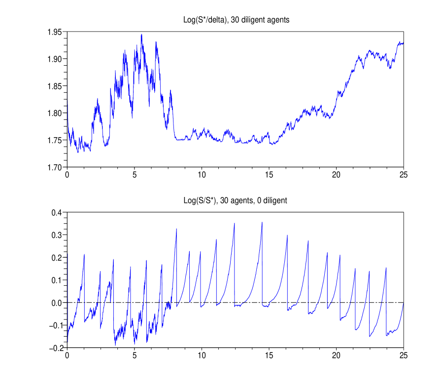
Figure 1:

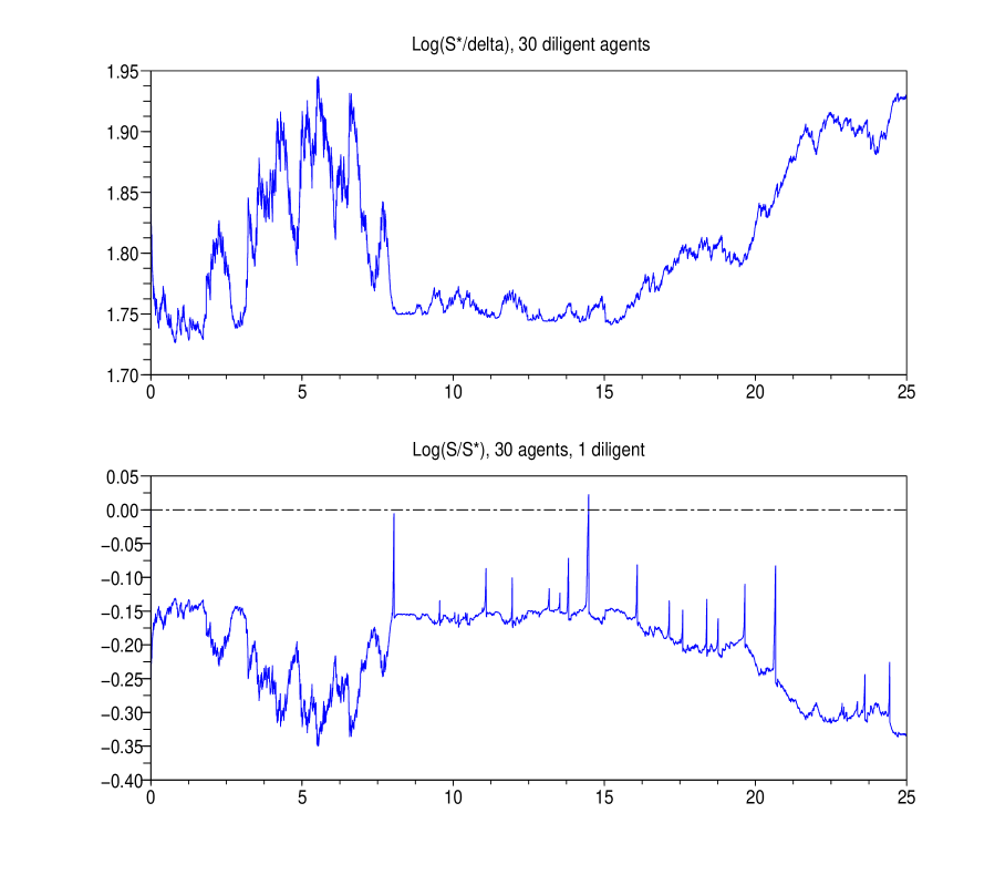
Figure 2:

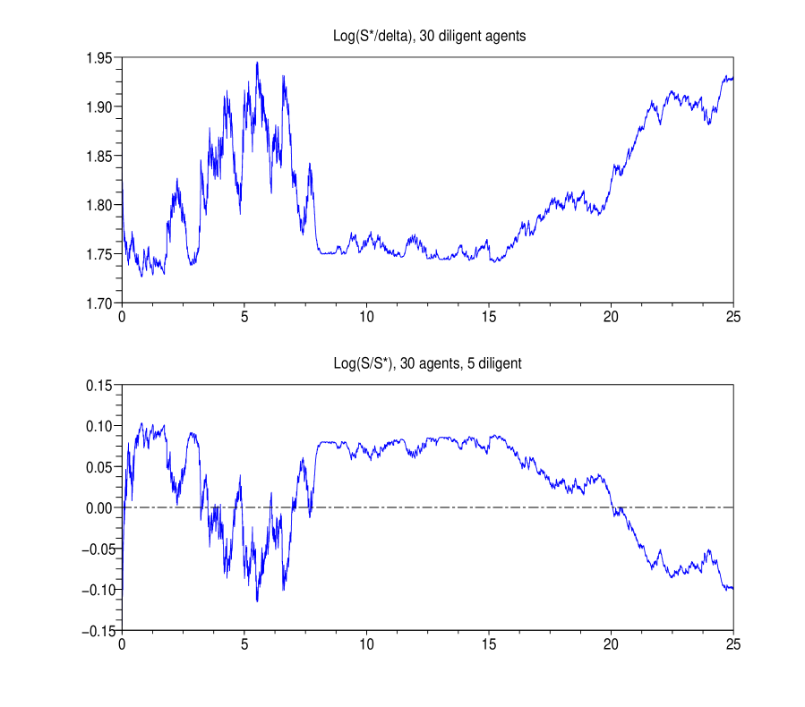
Figure 3:

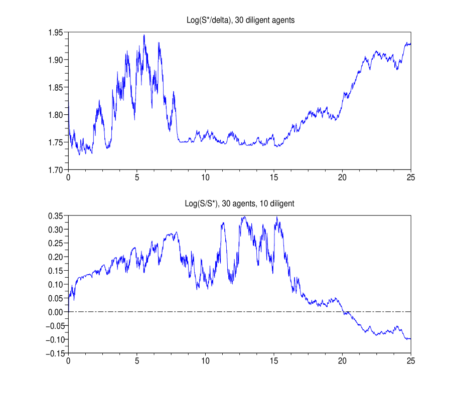
Figure 4:

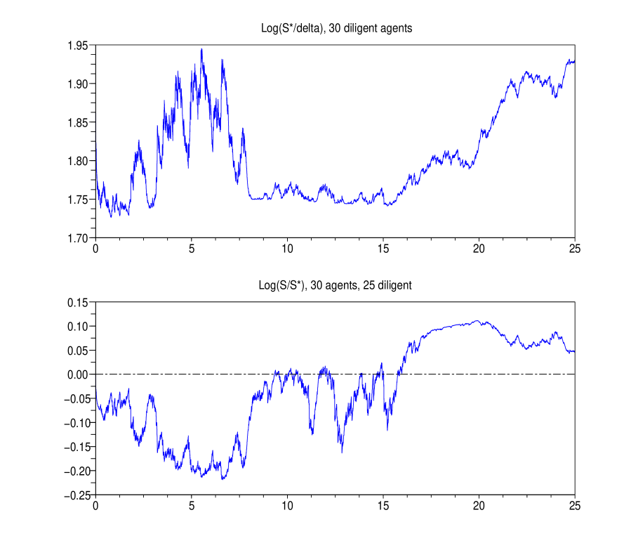
Figure 5:

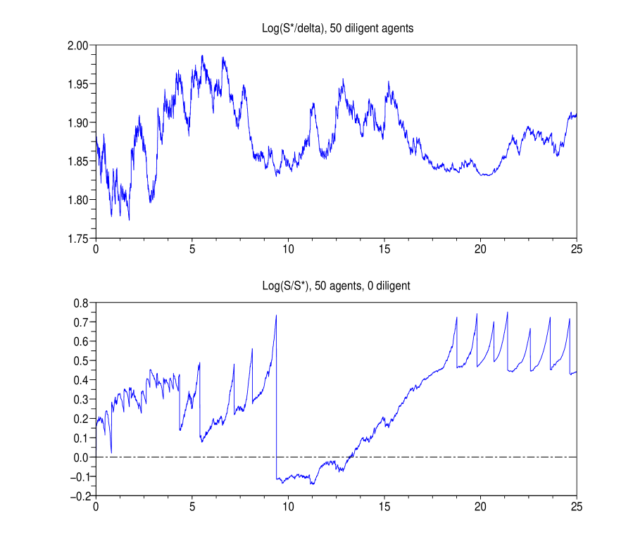
Figure 6:

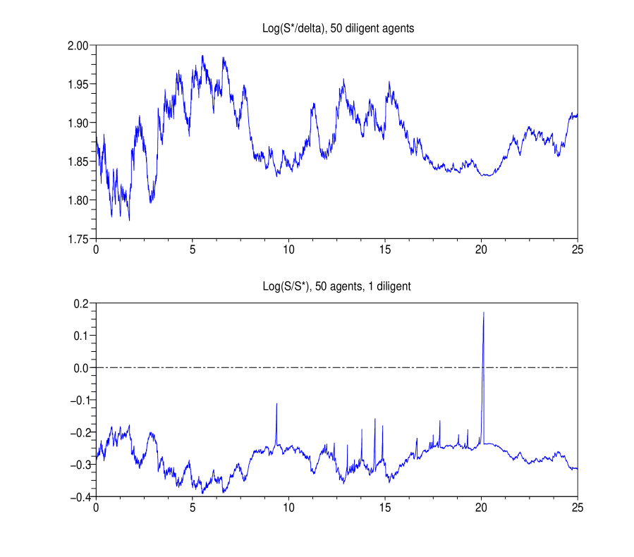
Figure 7:

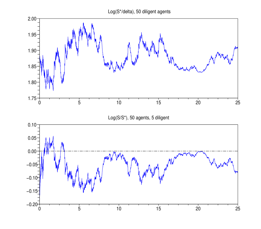
Figure 8:

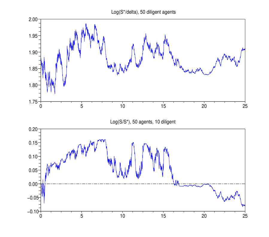
Figure 9:

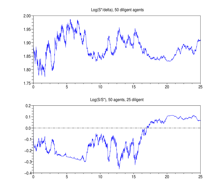
Figure 10:

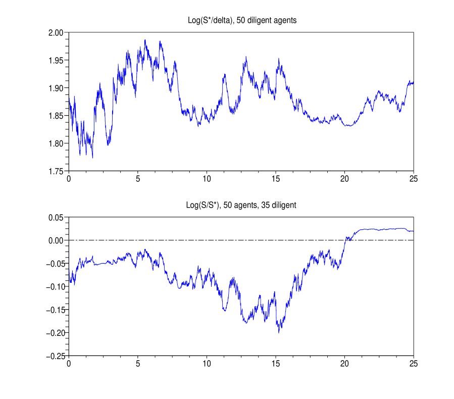
Figure 11:

Appendix C Proof of Theorem 2.3

There are several steps to the proof.

1. If we write ${\bar{\lambda}}^{j}_{t}\equiv U^{\prime}_{j}(t,{\bar{c}}^{j}_{t})$, the first thing to prove is that for $0\leq t<T$

   $${\bar{\lambda}}^{j}_{t}{\bar{S}}_{t}=E\left[{\bar{\lambda}}^{j}_{t+1}({\bar{S}}_{t+1}+\delta_{t+1})\ \Big{|}\ \bar{\cal{F}}^{j}_{t}\right].$$ (C.1)

   Consider a (small) perturbation ${\bar{\theta}}^{j}\mapsto{\bar{\theta}}^{j}+\eta$ of the portfolio process, with corresponding change ${\bar{c}}^{j}\mapsto c={\bar{c}}^{j}+\epsilon$ to the consumption process, where (see(2.2))

   $$\epsilon_{t}=\eta_{t}({\bar{S}}_{t}+\delta_{t})-\eta_{t+1}{\bar{S}}_{t}.$$

   Since $U$ satisfies the Inada condition, ${\bar{c}}^{j}$ must be strictly positive and so for small enough $\eta$ the process $c$ will be strictly positive. To leading order the change in agent $j$’s objective is

   $$E\Big{[}\sum^{T}_{t=0}U^{\prime}_{j}(t,{\bar{c}}^{j}_{t})\epsilon_{t}\Bigr{]} = E\Big{[}\sum^{T}_{t=0}{\bar{\lambda}}^{j}_{t}\{\eta_{t}({\bar{S}}_{t}+\delta_{t})-\eta_{t+1}{\bar{S}}_{t}\}\Big{]}$$ (C.2)

   $$= E\Big{[}\sum^{T}_{t=1}\eta_{t}({\bar{\lambda}}^{j}_{t}({\bar{S}}_{t}+\delta_{t})-{\bar{\lambda}}^{j}_{t-1}{\bar{S}}_{t-1})\Big{]}$$

   $$= E\Big{[}\sum^{T}_{t=1}\eta_{t}E({\bar{\lambda}}^{j}_{t}({\bar{S}}_{t}+\delta_{t})-{\bar{\lambda}}^{j}_{t-1}{\bar{S}}_{t-1}\,\big{|}\,\bar{{\cal F}}^{j}_{t-1})\Big{]},$$

   using the facts that ${\bar{S}}_{T}=0$, $\eta_{0}=0$ (since $\theta^{j}_{0}=y^{j}$ is fixed), and that the portfolio perturbation must be $\bar{{\cal F}}^{j}$-previsible. This leading-order change in objective must be $0$, since $({\bar{\theta}}^{j},{\bar{c}}^{j})$ was optimal; since $\eta$ is arbitrary, inspection of (C.2) gives (C.1).

2. Since ${\bar{c}}^{j}$ is $\bar{{\cal F}}^{j}$-adapted and ${\bar{\theta}}^{j}$ is $\bar{{\cal F}}^{j}$-previsible, we have

   $$\bar{{\cal F}}^{j}_{t} \equiv \sigma(X_{u},{\bar{S}}_{u},z^{j}_{u}\ :\ u\leq t)$$

   $$= \sigma(X_{u},{\bar{S}}_{u},{\bar{\theta}}^{j}_{u+1},{\bar{c}}^{j}_{u},z^{j}_{u}\ :\ u\leq t)$$

   $$\supseteq \sigma(X_{u},{\bar{S}}_{u},{\bar{\theta}}^{j}_{u+1},{\bar{c}}^{j}_{u}\ :\ u\leq t)\equiv{{\cal F}}^{j}_{t},$$

   say. Since ${\bar{\lambda}}^{j}_{t}$ and ${\bar{S}}_{t}$ are measurable with respect to ${{\cal F}}^{j}_{t}$, we can refine (C.1) to

   $${\bar{\lambda}}^{j}_{t}{\bar{S}}_{t}=E\Big{[}{\bar{\lambda}}^{j}_{t+1}({\bar{S}}_{t+1}+\delta_{t+1})\ \Big{|}\ {{\cal F}}^{j}_{t}\Big{]}.$$ (C.3)

3. We now take a regular conditional distribution $\kappa^{j}$ for ${\bar{S}}$ given $(X,{\bar{\theta}}^{j},{\bar{c}}^{j})$ - see II.89 in [43]. To build the sample space ${\tilde{\Omega}}$ on which the DB equilibrium will be constructed, the first step is to take $\Omega_{0}$ to be the path space of $(X,\Theta,C)$, which is isomorphic to $\mathbb{R}^{(d+2J)(T+1)}$. This gets its Borel $\sigma$-field ${\cal B}$, and canonical filtration; we endow it with a reference probability measure $P^{*}$ which is the law of $(X,{\bar{\Theta}},{\bar{C}})$. Next we expand the sample space to ${\tilde{\Omega}}\equiv\Omega_{0}\times\mathbb{R}^{T+1}$, and we write $(\tilde{X},{\tilde{\Theta}},\tilde{C})$ for the processes defined on ${\tilde{\Omega}}$ by

   $$\tilde{X}({\tilde{\omega}}) = X(\omega)$$

   $${\tilde{\Theta}}({\tilde{\omega}}) = \Theta(\omega)$$

   $$\tilde{C}({\tilde{\omega}}) = C(\omega),$$

   where ${\tilde{\omega}}=(\omega,s)$, $\omega\in\Omega_{0}$, $s=(s_{0},\dots,s_{T})\in\mathbb{R}^{T+1}$. We define a process $\tilde{S}$ by

   $$\tilde{S}_{t}({\tilde{\omega}})=s_{t}$$

   when ${\tilde{\omega}}=(\omega,(s_{0},\dots,s_{T}))$. We write $\tilde{{\cal G}}_{t}=\sigma(\tilde{X}_{u},{\tilde{\Theta}}_{u+1},\tilde{C}_{u},\tilde{S}_{u}:u\leq t)$ for the filtration generated by these processes.

   Now we specify the probabilities $P^{j}$ giving the diverse beliefs of the agents. Firstly, select $(\tilde{X},{\tilde{\theta}}^{j},\tilde{c}^{j})$ according to the law $P^{*}$ (equivalently, $(\tilde{X},{\tilde{\theta}}^{j},\tilde{c}^{j})$ has the same law as $(X,{\bar{\theta}}^{j},{\bar{c}}^{j})$). Then conditional on $(\tilde{X},{\tilde{\theta}}^{j},\tilde{c}^{j})$ let the law of $\tilde{S}$ be $\kappa^{j}(\tilde{X},{\tilde{\theta}}^{j},\tilde{c}^{j};\cdot)$, and let the random variables ${\tilde{\theta}}^{i},\tilde{c}^{i}$, $i\neq j$, be independent subject to the constraints $\sum{\tilde{\theta}}^{i}_{t}=1$, $\sum\tilde{c}^{i}_{t}=\delta_{t}$. [For example, we could take exponential variables $V^{i}$, $\tilde{V}^{j}$, and define ${\tilde{\theta}}^{i}_{t}=(1-{\tilde{\theta}}^{j}_{t})V^{i}/\sum_{\ell\neq j}V^{\ell}$, $\tilde{c}^{i}_{t}=(\tilde{\delta}_{t}-\tilde{c}^{j}_{t})\tilde{V}^{i}/\sum_{\ell\neq j}\tilde{V}^{\ell}$]. This construction has achieved the following properties:

4. (a) the $P^{j}$-distribution of $(\tilde{X},{\tilde{\theta}}^{j},\tilde{c}^{j},\tilde{S})$ is the same as the $P$-distribution of $(X,\bar{\theta}^{j},{\bar{c}}^{j},{\bar{S}})$;

5. (b) ${\tilde{\theta}}^{j}$ is $\tilde{{\cal G}}$-previsible.

6. (c)

   $${\tilde{\theta}}^{j}_{t}(\tilde{S}_{t}+\tilde{\delta}_{t})={\tilde{\theta}}^{j}_{t+1}\tilde{S}_{t}+\tilde{c}^{j}_{t}$$

   with $P^{j}$-probability 1, since this is a statement about the joint law of $(\tilde{X},{\tilde{\theta}}^{j},\tilde{c}^{j},\tilde{S})$ and it must therefore have the same probability as the corresponding statement about $(X,\bar{\theta}^{j},\bar{c}^{j},\bar{S})$;

7. (d) Similarly,

   $$\sum_{J}{\tilde{\theta}}^{i}_{t}=1,\quad\sum_{J}\tilde{c}^{i}_{t}=\tilde{\delta}_{t}$$

   with $P^{*}$-probability 1, and with $P^{k}$-probability 1 for each $k$.

8. Now we define the filtration $\tilde{{\cal F}}^{j}_{t}=\sigma(\tilde{X}_{u},\tilde{S}_{u},{\tilde{\theta}}^{j}_{u+1},\tilde{c}^{j}_{u}\ :\ u\leq t)$, and the processes ${\tilde{\lambda}}^{j}_{t}\equiv U^{\prime}_{j}(t,\tilde{c}^{j}_{t})$. Hence we observe the analogue

   $${\tilde{\lambda}}^{j}_{t}\tilde{S}_{t}=E^{j}\Big{[}{\tilde{\lambda}}^{j}_{t+1}(\tilde{S}_{t+1}+\tilde{\delta}_{t+1})\Big{|}\tilde{{\cal F}}^{j}_{t}\Big{]}$$ (C.4)

   of (C.3) must hold, because the conditional expedition is determined by the joint law of the conditional and conditioning variables, which (in view of (a)) is the same as the joint law of the corresponding variable in the PI equilibrium for which (C.3) holds.

9. The next step is to argue that (C.3) holds when we condition on the larger $\sigma$-field $\tilde{{\cal G}}_{t}$:

   $${\tilde{\lambda}}^{j}_{t}\tilde{S}_{t}=E^{j}\Big{[}{\tilde{\lambda}}^{j}_{t+1}(\tilde{S}_{t+1}+\delta_{t+1})\Big{|}\tilde{{\cal G}}_{t}\Big{]}.$$ (C.5)

   But $\tilde{{\cal G}}_{t}=\tilde{{\cal F}}^{j}_{t}\ \vee\ {{\cal A}}^{j}_{t}$, where ${{\cal A}}^{j}_{t}=\sigma(\tilde{c}^{i}_{u},{\tilde{\theta}}^{i}_{u+1}\ :\ u\leq t,\ i\neq j)$ is independent of $\tilde{{\cal F}}^{j}_{t}$ so we may apply Proposition 2 to deduce this result.

10. The final step is to verify the optimality property (v) in the definition of a DB equilibrium. Suppose for this that $(\theta_{t},c_{t})$ is any possible investment-consumption pair for agent $j$ (so $\theta_{0}=y^{j}$, $\theta$ is $\tilde{{\cal G}}$-previsible, $c$ is $\tilde{{\cal G}}$-adapted, $\theta_{t}(\tilde{S}_{t}+\delta_{t})=\theta_{t+1}\tilde{S}_{t}+c_{t}$ for all $t$) and consider the objective

    $$E^{j}\sum^{T}_{t=0}U_{j}(t,c_{t}) \leq E^{j}\sum^{T}_{t=0}\Big{[}U_{j}(t,\tilde{c}^{j}_{t})+{\tilde{\lambda}}^{j}_{t}(c_{t}-\tilde{c}^{j}_{t})\Big{]}$$

    $$= E^{j}\sum^{T}_{t=0}\Big{[}U_{j}(t,\tilde{c}^{j}_{t})+{\tilde{\lambda}}^{j}_{t}\Big{\{}(\theta_{t}-{\tilde{\theta}}^{j}_{t})(\tilde{S}_{t}+\tilde{\delta}_{t})-(\theta_{t+1}-{\tilde{\theta}}^{j}_{t+1})\tilde{S}_{t}\Big{\}}\Big{]}$$

    $$= E^{j}\sum^{T}_{t=0}U_{j}(t,\tilde{c}^{j}_{t})+E\sum^{T}_{t=1}(\theta_{t}-{\tilde{\theta}}^{j}_{t})\Big{\{}{\tilde{\lambda}}^{j}_{t}(\tilde{S}_{t}+\tilde{\delta}_{t})-{\tilde{\lambda}}^{j}_{t-1}\tilde{S}_{t_{1}}\Big{\}}$$

    $$= E^{j}\sum^{T}_{t=0}U_{j}(t,\tilde{c}^{j}_{t})$$

    using (respectively) concavity of $U_{j}$, the wealth equation, the fact that $\theta_{0}={\tilde{\theta}}^{j}_{0}=y^{j}$ and $\theta_{T+1}=0={\tilde{\theta}}^{j}_{T+1}$, and (C.4) together with $\tilde{{\cal G}}$-previsibility of $\theta$, ${\tilde{\theta}}^{j}$.

    $\square$

We give here a simple and intuitive result that was needed in the proof of Theorem 2.3.

Proposition 2.

If $X$ is an integrable random variable, if ${\cal G}$ and ${\cal A}$ are two sub-$\sigma$-fields of ${\cal F}$ such that ${\cal A}$ is independent of $X$ and ${\cal G}$, then

$$E[X|{\cal G}]=E[X|{\cal G}\vee{\cal A}]\qquad\hbox{\rm a.s.}$$ (C.6)

Proof of Proposition 2. Consider the collection

$${\cal C}\equiv\{F\in{\cal F}:\int_{F}\,E[X|{\cal G}]\;dP=\int_{F}\,X\;dP\}.$$

This collection is a $d$-system (see [43] Chapter II.1 for definitions and basic results). From the definition of conditional expectation, ${\cal G}\subseteq{\cal C}$. Now take any $G\in{\cal G}$, $A\in{\cal A}$ and calculate

$$\int_{A\cap G}\,E[X|{\cal G}]\;dP = \int I_{A}E[XI_{G}|{\cal G}]\;dP$$

$$= P(A)E[X:G]\qquad(\hbox{\rm${\cal A}$ is independent of ${\cal G}$})$$

$$= \int_{A\cap G}X\;dP\qquad(\hbox{\rm${\cal A}$ is independent of ${\cal G}$, $X$}).$$

Thus ${\cal C}$ contains the $\pi$-system ${\cal I}$ consisting of all intersections of the form $A\cap G$, $A\in{\cal A}$, $G\in{\cal G}$, and by Lemma II.1.8 of [43], the $d$-system $d({\cal I})$ generated by ${\cal I}$ equals the $\sigma$-field generated by ${\cal I}$, which is ${\cal G}\vee{\cal A}$. But ${\cal C}$ is a $d$-system, and so contains ${\cal G}\vee{\cal A}$. This establishes the result. $\square$

Remark. Intuitively, it seems plausible that we should not need ${\cal A}$ to be independent of ${\cal G}$ for this result to hold; after all, what we are adding to the $\sigma$-field is independent of the random variable. But this is not true. Take the example of two independent $B(1,{\scriptstyle\frac{1}{2}})$ random variables $X$ and $Y$, and let ${\cal A}=\sigma(Y)$, ${\cal G}=\sigma(Z)$ where $Z=(X+Y)\mod(2)$. Thus $Z$ is 1 if exactly one of $X$, $Y$ is 1, zero otherwise. It is not hard to see that ${\cal G}$ is independent of $X$, and yet ${\cal A}\vee{\cal G}={\cal F}$, so the equality (C.6) fails.

References

- [1] Allen, F., Morris, S., and Shin, H. Beauty contests and iterated expectations in asset markets. Review of Financial Studies 19 (2006), 719–752.
- [2] Angeletos, G. M., and Pavan, A. Efficient use of information and social value of information. Tech. rep., MIT, 2006.
- [3] Basak, S. A model of dynamic equilibrium asset pricing with heterogeneous beliefs and extraneous risk. Journal of Economic Dynamics & Control 24 (2000), 63–95.
- [4] Basak, S. Asset pricing with heterogeneous beliefs. Journal of Banking and FInance 29 (2005), 2849–2881.
- [5] Basak, S., and Croitoru, B. Equilibrium mispricing in a capital market with portfolio constraints. Review of Financial Studies 13 (2000), 715–748.
- [6] Bawa, V. S., Brown, S. J., and Klein, R. W. Estimation risk and optimal portfolio choice. North-Holland, Amsterdam, 1979.
- [7] Brennan, M. J., and Xia, Y. Stock price volatility and equity premium. Journal of Monetary Economics 7 (2001), 265–296.
- [8] Brown, A. A. A note on heterogeneous beliefs with CRRA utilities. Preprint, Statistical Laboratory, University of Cambridge, arXiv:0907.4964v1, 2009.
- [9] Brown, A. A., and Rogers, L. C. G. Heterogeneous beliefs with finite-lived agents. arXiv:0907.4953, 2009.
- [10] Brown, D., and Jennings, R. On technical analysis. Review of Financial Studies 2 (1989), 527–551.
- [11] Buraschi, A., and Jiltsov, A. Model uncertainty and option markets with heterogeneous beliefs. Journal of Finance 61, 6 (2006), 2841–2897.
- [12] Cabrales, A., and Hoshi, T. Heterogeneous beliefs, wealth accumulation and asset price dynamics. Journal of Economic Dynamics and Control 20 (1996), 1073–1100.
- [13] Calvet, L., Grandmont, J.-M., and Lemaire, I. Aggregation of heterogeneous beliefs, asset pricing and risk sharing in complete financial markets. Tech. rep., CREST, 2001.
- [14] David, A., and Veronesi, P. Option Prices with Uncertain Fundamentals: Theory and Evidence on the Dynamics of Implied Volatilities. Working paper (2000).
- [15] De Long, J. B., Shleifer, A., Summers, L. H., and Waldmann, R. J. Noise trader risk in financial markets. Journal of Political Economy 98 (1990), 703–738.
- [16] Detemple, J., and Murthy, S. Intertemporal asset pricing with heterogeneous beliefs. Journal of Economic Theory 62 (1994), 294–320.
- [17] Diamond, D., and Verrecchia, R. Information aggregation in a noisy rational expectations equilibrium. Journal of Financial Economics 9 (1981), 221–235.
- [18] Fan, M. Heterogeneous beliefs, the term structure and time-varying risk premia. Annals of Finance 2 (2006), 259–285.
- [19] Gallmeyer, M., and Hollifield, B. An examination of heterogeneous beliefs with a short-sale constraint in a dynamic economy. Tech. rep., SSRN, 2007.
- [20] Grossman, S. J., and Stiglitz, J. On the impossibility of informationally efficient markets. American Economic Review 70 (1980), 393–408.
- [21] Grundy, B., and McNichols, M. Trade and revelation of information through prices and direct disclosure. Review of Financial Studies 2 (1989), 495–526.
- [22] Guidolin, M., and Timmermann, A. Option prices under bayesian learning: Implied volatility dynamics and predictive densities. Working paper (2001).
- [23] Harris, M., and Raviv, A. Differences of opinion make a horse race. Review of Financial Studies 6 (1993), 473–506.
- [24] Harrison, J. M., and Kreps, D. Speculative investor behavior in a stock market with heterogeneous expectations. Quarterly Journal of Economics 92 (1978), 323–336.
- [25] He, H., and Wang, J. Differential information and dynamic behaviour of stock trading. Review of Financial Studies 8 (1995), 914–972.
- [26] Hellwig, C. Public announcements, adjustment delays and the business cycle. Tech. rep., Department of Economics, UCLA, 2002.
- [27] Hellwig, C. Heterogeneous information and welfare effects of public information. Tech. rep., Department of Economics, UCLA, 2005.
- [28] Jobert, A., Platania, A., and Rogers, L. C. G. A Bayesian solution to the equity premium puzzle. Preprint, Statistical Laboratory, University of Cambridge, 2006.
- [29] Jouini, E., and Napp, C. Consensus consumer and intertemporal asset pricing with heterogeneous beliefs. Review of Economic Studies 74 (2007), 1149–1174.
- [30] Judd, K. L., and Bernardo, A. E. Asset market equilibrium with general tastes, returns, and informational asymmetries. Journal of Financial Markets 1 (2000), 17–43.
- [31] Kandel, E., and Pearson, N. D. Differential interpretation of public signals and trade in speculative markets. Journal of Political Economy 4 (1995), 831–872.
- [32] Keynes, J. The General Theory of Employment, Interest and Money. Macmillan, 1936.
- [33] Kogan, L., Ross, S., Wang, J., and Westerfield, M. M. Market selection. Tech. rep., NBER Working Paper Series, 2009.
- [34] Kurz, M. Rational Diverse Beliefs and Economic Volatility. Prepared for the Handbook of Finance Series Volume Entitled: Handbook of Financial Markets: Dynamics and Evolution (2008).
- [35] Kurz, M., Jin, H., and Motolese, M. Determinants of stock market volatility and risk premia. Annals of Finance 1, 2 (2005), 109–147.
- [36] Leland, H. E. Who should buy portfolio insurance? Journal of Finance 35, 2 (1980), 581–94.
- [37] Li, T. M., and Rogers, L. C. G. A doubly bayesian approach to the equity premium puzzle. Preprint, Statistical Laboratory, University of Cambridge, 2009.
- [38] Li, T. M., and Rogers, L. C. G. Lucas economy with trading constraints. Preprint, Statistical Laboratory, University of Cambridge, 2009.
- [39] Lucas, R. E. Expectations and the neutrality of money. Journal of Economic Theory 4 (1972), 103–124.
- [40] Morris, S., and Shin, H. S. Social value of public information. American Economic Review 92 (2002), 1521–1534.
- [41] Morris, S., and Shin, H. S. Central bank transparency and the signal value of prices. Brookings Papers on Econonic Activity 2 (2005), 1–66.
- [42] Rogers, L. C. G. The relaxed investor and parameter uncertainty. Finance and Stochastics 5 (2001), 131–154.
- [43] Rogers, L. C. G., and Williams, D. Diffusions, Markov Processes and Martingales. Cambridge University Press, 2000.
- [44] Scheinkman, J., and Xiong, W. Overconfidence and speculative bubbles. Journal of Political Economy 111 (2005), 1183–1219.
- [45] Singleton, K. Asset prices in a time-series model with disparately informed, competitive traders. In New Approaches to Monetary Economics: Proceedings of the Second International Symposium in Economic Theory and Econometrics (1987), W. Barnet and K. Singleton, Eds., Cambridge University Press.
- [46] Townsend, R. Market anticipations, rational expectations and Bayesian analysis. International Economic Review 19 (1978), 481–494.
- [47] Varian, H. R. Divergence of opinion in complete markets: a note. Journal of Finance 40 (1985), 309–317.
- [48] Varian, H. R. Differences of opinion in financial markets. In Financial Risk: Theory, Evidence and Implications (Boston, 1989), C. C. Stone, Ed., Kluwer Academic Publishers.
- [49] Wang, J. A model of competitive stock trading volume. Journal of Political Economy 102 (1994), 127–167.
- [50] Weizmann, M. A unified Bayesian theory of equity puzzles. Preprint, Harvard University, 2005.
- [51] Wu, H. M., and Guo, W. C. Speculative trading with rational beliefs and endogenous uncertainty. Economic Theory 21 (2003), 263–292.
- [52] Wu, H. M., and Guo, W. C. Asset price volatility and trading volume with rational beliefs. Economic Theory 23 (2004), 795–829.