Fluctuation-dissipation relations and field-free algorithms for the computation of response functions

Abstract

We discuss the relation between the fluctuation-dissipation relation derived by Chatelain and Ricci-Tersenghi [C.Chatelain, J.Phys. A 36, 10739 (2003); F. Ricci-Tersenghi, Phys.Rev.E 68, 065104(R) (2003)] and that by Lippiello-Corberi-Zannetti [E. Lippiello, F. Corberi and M. Zannetti Phys. Rev. E 71, 036104 (2005)]. In order to do that, we re-derive the fluctuation-dissipation relation for systems of discrete variables evolving in discrete time via a stochastic non-equilibrium Markov process. The calculation is carried out in a general formalism comprising the Chatelain, Ricci-Tersenghi result and that by Lippiello-Corberi-Zannetti as special cases. The applicability, generality, and experimental feasibility of the two approaches is thoroughly discussed. Extending the analytical calculation to the variance of the response function we show the vantage of field-free numerical methods with respect to the standard method where the perturbation is applied. We also show that the signal to noise ratio is better (by a factor $\sqrt{2}$) in the algorithm of Lippiello-Corberi-Zannetti with respect to that of Chatelain-Ricci Tersenghi.

PACS: 05.70.Ln, 75.40.Gb, 05.40.-a

I Introduction

Recently, there has been much interest in the extension in the out of equilibrium regime of the fluctuation-dissipation theorem (FDT), through more general fluctuation-dissipation relation (FDR), which have led to the concept of effective temperature efftemp and to the connection between non-equilibrium and equilibrium properties fmpp . Fluctuating two-time quantities have also been actively investigated, particularly in relation to the detection and quantification of dynamical heterogeneities, mostly in disordered systems c4 .

The search of FDR between response functions and properties of the unperturbed system, has led to a number of proposals CKP ; Crisanti ; chatelain ; rt ; lcz ; Diez ; Berthier ; noi_nonlin ; noi_nonlin2 . Among these, the two by Chatelain chatelain and Ricci-Tersenghi rt (CRT) and the one by Lippiello, Corberi, Zannetti lcz ; noi_nonlin ; noi_nonlin2 (LCZ) have succeeded in making the connection between the dynamical susceptibility and unperturbed correlators between observable quantities. In addition to the intrinsic theoretical interest, these results opened the way to the development of perturbation-free numerical algorithms, allowing for highly efficient and precise measurements of the response function via correlators, without need of switching on any perturbation.

However, the paths followed by CRT on one side and by LCZ on the other, are quite different as well as the final results. The two approaches lead to expressions of the susceptibility in terms of radically different unperturbed correlation functions, making the mapping between them cumbersome. This poses the question of understanding the inner relationship between the two results, of their degree of generality, of which is performing better in numerical implementations and of the possible experimental implications. In this paper we study these issues and answer these questions. In order to carry out this program, we derive the FDR for systems evolving in discrete time via stochastic Markov processes, defined by transition probabilities obeying detailed balance. We develop a unified formalism containing different approaches as special cases and explain the difference between those of CRT and LCZ: while in the LCZ case the response function is related to correlation functions computed over the whole non-equilibrium ensemble, in the CRT approach, instead, averages are taken over a restricted set of trajectories.

The derivation is fully general for what concerns the nature of the discrete variables (e.g. Ising, Potts, Clock etc.) and of the transition probabilities. However, the constraint of a restricted set of trajectories in the CRT approach requires the microscopic knowledge of the sequence of (attempted) updates, which is manageable only in numerical simulations. On the other hand, in the LCZ approach a standard unrestricted ensemble average is involved, and the response function is written in terms of standard correlation functions between observable quantities. This allows analytical treatments by means of the usual methods of statistical mechanics and, in principle, experimental applications. On the other hand, other approaches, such as those in Crisanti ; Diez ; Berthier do not express the response function in terms of observables.

After clarifying the relations between the FDR in the CRT and LCZ approaches, we turn to compare the efficiencies of the numerical algorithms based on them, together with that of the standard method (SM), requiring the application of an external perturbation $h$. An important advantage of the perturbation-free methods is that the limit $h\to 0$ is built in, while, with the SM, checking for linearity is often numerically demanding. Besides this, field-free methods are also characterized by a better signal to noise ratio. This is a relevant fact, since the numerical computation of the response function is extremely noisy. In order to quantify such a noise, we compute exactly the variance of the response function for each of the three algorithms. In the SM it diverges as $1/h^{2}$, preventing small values of $h$ to be used and making linearity often insecure. Since, obviously, such a drawback is absent with the field-free methods, there is an enormous advantage in their implementation. Nevertheless, also with perturbation-free algorithms the noise can be significant, especially for large time differences. The comparison between the variances of the CRT and the LCZ methods shows that the LCZ approach yields a better signal to noise ratio by a factor $\sqrt{2}$. Basically, this difference is a consequence of the restriction in the set of trajectories required by the CRT method.

In addition to the relevance for numerical applications, the results for the variances give a contribution to the understanding of fluctuations of two-time quantities, shedding some light in the field of nonlinear susceptibilities bb .

After investigating and clarifying the relation between the different algorithms and their performances, we present the results of numerical simulations in order to discuss the generality of the method and to illustrate the efficiency of the field-free algorithms with particular examples. We compute numerically the response function for models of Ising spins (the ferromagnetic Ising model and the Edwards-Anderson (EA) spin glass in $d=3$) with the three methods. We show that both the CRT and the LCZ algorithms produce, with great accuracy, the same response which can be obtained with the SM. Computing the variances of the three methods, we obtain the results outlined above. Finally, we compute the response function in the Fredrickson-Andersen (FA) model, both applying the perturbation and with the field-free method of LCZ, finding again perfect agreement. This demonstrates the applicability of the LCZ algorithm also in this case, and that the criticism raised in Ref. mayersollich does not hold.

This Article is organised as follows: In Sec. II we present the derivation of the FDR. We discuss the results obtained, their generality and the measurability of the correlators involved. In Sec. III we compute and compare the variances of the three algorithms. Sec. IV is devoted to explicit numerical implementations: We consider the $3d$ ferromagnetic Ising and EA models quenched to the critical temperature and below it. Sec. IV.2 contains the application to the FA model. The conclusions are drawn in Sec. V, where some perspectives are discussed.

II Analytical derivation of fluctuation-dissipation relations

We consider a system of $N$ discrete variables $\sigma_{i}$ (i.e. those entering models as Ising, Potts, Clock etc …), generically called spins. Time $t$ is discretized, namely $t_{n}=n\delta$, where $n$ is an integer, and the time-step is $\delta=1/N$. A configuration update is attempted at each time step.

II.1 Transition probabilities

Spin variables evolve in discrete time according to a generic Markov chain regulated by the transition probabilities $w(\sigma^{\prime\prime}|\sigma^{\prime},n)$ to go from a configuration $\sigma^{\prime}$ to another $\sigma^{\prime\prime}$ in the $n$-th time-step. Transition probabilities obey the instantaneous detailed balance

$$w(\sigma^{\prime\prime}|\sigma^{\prime},n)\exp[-\beta{\cal H}(\sigma^{\prime},n)]=w(\sigma^{\prime}|\sigma^{\prime\prime},n)\exp[-\beta{\cal H}(\sigma^{\prime\prime},n)],$$ (1)

where ${\cal H}(\sigma,n)$ is the (time dependent) Hamiltonian of the system. The diagonal terms $w(\sigma^{\prime}|\sigma^{\prime},n)$ remain fixed by the normalization condition

$$w(\sigma^{\prime}|\sigma^{\prime},n)=1-\sum_{\tilde{\sigma}\neq\sigma^{\prime}}w(\tilde{\sigma}|\sigma^{\prime},n).$$ (2)

Restricting, for simplicity, to the case of single spin update, the form of the transition probabilities at time $n$ is

$$w(\sigma^{\prime\prime}|\sigma^{\prime},n)=\frac{1}{N}\sum_{k}w_{k}(\sigma^{\prime\prime}|\sigma^{\prime},n),$$ (3)

where $w_{k}$ are the single-spin transition probabilities, namely $\sigma^{\prime\prime}$ and $\sigma^{\prime}$ may differ only for the $k$-th spin.

The two-time conditional probability $P(\sigma,n|\sigma^{\prime},m)$ to go from $\sigma^{\prime}$ at time $m$ to $\sigma$ at time $n$ can be expressed as

$$P(\sigma,n|\sigma^{\prime},m)=\frac{1}{N^{n-m}}\sum_{i_{n-1},\ldots,i_{m}}\sum_{\sigma^{(n-1)},\ldots,\sigma^{(m+1)}}w_{i_{n-1}}\left(\sigma|\sigma^{(n-1)},n\right)\ldots w_{i_{m}}\left(\sigma^{(m+1)}|\sigma^{\prime},m\right).$$ (4)

In the case of time independent $w$, the conditional probability is time translation invariant. For later use, we write this property as

$$P(\sigma,n|\sigma^{\prime},m+1)=P(\sigma,n-1|\sigma^{\prime},m).$$ (5)

Given two generic observables $A(\sigma)$ and $B(\sigma)$ (namely functions of a configuration of the system), from the knowledge of the conditional probability one can compute their correlation function

$$C_{AB}(n,m)=\langle A(n)B(m)\rangle=\sum_{\sigma,\sigma^{\prime}}A(\sigma)P(\sigma,n|\sigma^{\prime},m)B(\sigma^{\prime})P(\sigma^{\prime},m).$$ (6)

II.2 Relation between perturbed and unperturbed transition probabilities

In the presence of an external perturbation $h_{j}(n)$ switched-on in the $j$-th site, the evolution is controlled by the Hamiltonian ${\cal H}(\sigma,n)={\cal H}_{0}(\sigma)-\sigma_{j}h_{j}(n)$. In the following we will always consider time-independent unperturbed transition probabilities and we will drop the time dependence in the unperturbed transition rates. The detailed balance condition (1) for the perturbed transition probabilities reads

$$\frac{w_{j}^{h}(\sigma^{\prime\prime}|\sigma^{\prime},n)}{w_{j}^{h}(\sigma^{\prime}|\sigma^{\prime\prime},n)}=\frac{e^{-\beta{\cal H}_{0}(\sigma^{\prime\prime})}}{e^{-\beta{\cal H}_{0}(\sigma^{\prime})}}e^{\beta h_{j}(n)(\sigma_{j}^{\prime\prime}-\sigma_{j}^{\prime})},$$ (7)

where, from now on, $w_{j}$ and $w_{j}^{h}$ refer to unperturbed and perturbed transition probabilities, respectively. The most general form of $w^{h}_{j}$ obeying Eq. (7) is

$$w_{j}^{h}(\sigma^{\prime\prime}|\sigma^{\prime},n)=w_{j}(\sigma^{\prime\prime}|\sigma^{\prime},n)e^{\frac{\beta}{2}h_{j}(n)(\sigma^{\prime\prime}_{j}-\sigma^{\prime}_{j})}M_{j}(\sigma^{\prime},\sigma^{\prime\prime},n),$$ (8)

where $M_{j}(\sigma^{\prime},\sigma^{\prime\prime},n)$ is an $h$-dependent function symmetric with respect to the exchange of its arguments and such that $w_{j}^{h}$ is a probability, namely positive and normalizable. To linear order in the external perturbation one has

$$w_{j}^{h}(\sigma^{\prime\prime}|\sigma^{\prime},n) = w_{j}(\sigma^{\prime\prime}|\sigma^{\prime})\left[1-\frac{\beta}{2}h_{j}(n)(\sigma_{j}^{\prime}-\sigma_{j}^{\prime\prime})+m_{j}(\sigma^{\prime\prime},\sigma^{\prime})h_{j}(n)\right](1-\delta_{\sigma^{\prime},\sigma^{\prime\prime}})$$ (9)

$$+ \left\{1-\sum_{\tilde{\sigma}\neq\sigma^{\prime}}w_{j}(\tilde{\sigma}|\sigma^{\prime},n)\left[1-\frac{\beta}{2}h_{j}(n)(\sigma_{j}^{\prime}-\tilde{\sigma}_{j})+m_{j}(\tilde{\sigma},\sigma^{\prime},n)h_{j}(n)\right]\right\}\delta_{\sigma^{\prime},\sigma^{\prime\prime}}$$

where

$$m_{j}(\sigma^{\prime\prime},\sigma^{\prime},n)=\left.\frac{\partial M_{j}(\sigma^{\prime\prime},\sigma^{\prime},n)}{\partial h_{j}(n)}\right|_{h=0}.$$ (10)

Let us comment on $m_{j}$: It is well known that the detailed balance condition leaves an arbitrariety on the choice of the transition probabilities, both for the unperturbed and the perturbed ones. Even for a fixed choice of unperturbed $w_{j}$, therefore, there is a family of different $w_{j}^{h}$ obeying detailed balance, parametrized by $m_{j}$.

II.3 Response function

For a magnetic perturbing field $h_{j}(m)$ turned on the site $j$ in the $m$-th time-step the impulsive response function $R_{i,j}(n,m)$, describing the effect of the perturbation on the spin $\sigma_{i}$ at time $n>m$, is defined by

$$R_{i,j}(n,m)=\frac{1}{\delta}\left.\frac{\partial\langle\sigma_{i}(n)\rangle}{\partial h_{j}(m)}\right|_{h=0}=N\left.\frac{\partial\langle\sigma_{i}(n)\rangle}{\partial h_{j}(m)}\right|_{h=0},$$ (11)

where averages $\langle\ldots\rangle$ are taken over thermal histories and the initial condition.

From Eq.(4), one has

$$R_{i,j}(n,m)=N\sum_{\sigma,\sigma^{\prime},\sigma^{\prime\prime}}\sigma_{i}P(\sigma,n|\sigma^{\prime\prime},m+1)\left.\frac{dw^{h}_{j}\left(\sigma^{\prime\prime}|\sigma^{\prime}\right)}{dh_{j}}\right|_{h=0}P(\sigma^{\prime},m).$$ (12)

The derivative of the $w_{k}^{h}$ with respect to the field can be easily obtained from Eq.(9)

$$\left.\frac{\partial w_{j}^{h}(\sigma^{\prime\prime}|\sigma^{\prime},n)}{\partial h_{j}(m)}\right|_{h=0}=w_{j}(\sigma^{\prime\prime}|\sigma^{\prime})\left[f_{j}(\sigma^{\prime\prime},\sigma^{\prime})(1-\delta_{\sigma^{\prime},\sigma^{\prime\prime}})+g_{j}(\sigma^{\prime})\delta_{\sigma^{\prime},\sigma^{\prime\prime}}\right]\delta_{n,m}$$ (13)

where

$$f_{j}(\sigma^{\prime\prime},\sigma^{\prime})=-\frac{\beta}{2}(\sigma^{\prime}_{j}-\sigma^{\prime\prime}_{j})+m_{j}(\sigma^{\prime\prime},\sigma^{\prime}),$$ (14)

and

$$g_{j}\left(\sigma\right)w_{j}\left(\sigma|\sigma\right)=-\sum_{\sigma^{\prime}\neq\sigma}w_{j}\left(\sigma^{\prime}|\sigma\right)f_{j}\left(\sigma^{\prime},\sigma\right).$$ (15)

From Eqs. (13,14,15) it is clear that the response function of Eq. (12) cannot be straightforwardly interpreted as correlation functions. In order to do that, one would need the full transition probability $P(\sigma,n|\sigma^{\prime\prime},m+1)w(\sigma^{\prime\prime}|\sigma^{\prime},m)$ connecting $\sigma^{\prime}$ at time $m$ to $\sigma^{\prime\prime}$ at time $n$, with $w(\sigma^{\prime\prime}|\sigma^{\prime},m)$ containing all the $w_{k}(\sigma^{\prime\prime}|\sigma^{\prime})$ according to Eq.(3), while in Eqs. (13) only the one site $w_{j}(\sigma^{\prime\prime}|\sigma^{\prime})$ appears. A way out is to insert the missing $w(\sigma^{\prime\prime}|\sigma^{\prime},m)$ by writing $Ndw^{h}_{j}/dh_{j}|_{h=0}=dw^{h}/dh_{j}|_{h=0}=wd(\ln w^{h})/dh_{j}|_{h=0}$, as proposed in Berthier , obtaining

$$R_{i,j}(n,m)=\sum_{\sigma,\sigma^{\prime},\sigma^{\prime\prime}}\sigma_{i}P(\sigma,n|\sigma^{\prime\prime},m+1)w(\sigma^{\prime\prime}|\sigma^{\prime})\left.\frac{d\ln w^{h}\left(\sigma^{\prime\prime}|\sigma^{\prime}\right)}{dh_{j}}\right|_{h=0}P(\sigma^{\prime},m).$$ (16)

However, let us notice that, although the response function is expressed in terms of the unperturbed dynamics, the function appearing on the r.h.s. of Eq. (16) is not in the form of a correlation function between observables according to the definition (6). This is because $d(\ln w^{h})/dh_{j}|_{h=0}$ depends on two configurations.

Going back to Eq. (12), in order to illustrate the CRT and the LCZ approaches, it is useful to write the response function as the sum of an off-diagonal contribution $\overline{D}_{i,j}(n,m)$ and a diagonal contribution $D_{i,j}(n,m)$

$$R_{i,j}(n,m)=\overline{D}_{i,j}(n,m)+D_{i,j}(n,m)$$ (17)

with

$$\overline{D}_{i,j}(n,m)=N\sum_{\sigma,\sigma^{\prime},\sigma^{\prime\prime}}\sigma_{i}P(\sigma,n|\sigma^{\prime\prime},m+1)w_{j}\left(\sigma^{\prime\prime}|\sigma^{\prime}\right)f_{j}\left(\sigma^{\prime\prime},\sigma^{\prime}\right)\left[1-\delta_{\sigma^{\prime\prime},\sigma^{\prime}}\right]P(\sigma^{\prime},m)$$ (18)

and

$$D_{i,j}(n,m)=N\sum_{\sigma,\sigma^{\prime},\sigma^{\prime\prime}}\sigma_{i}P(\sigma,n|\sigma^{\prime\prime},m+1)w_{j}\left(\sigma^{\prime\prime}|\sigma^{\prime}\right)g_{j}\left(\sigma^{\prime}\right)\delta_{\sigma^{\prime\prime},\sigma^{\prime}}P(\sigma^{\prime},m).$$ (19)

The above equations are exact and fully general. The next step is to express $D_{i,j}$ and $\overline{D}_{i,j}$ in terms of correlation functions of observable quantities. This can be done in two different ways, leading to the CRT and LCZ results. We describe them separately below.

II.4 CRT class algorithms

Given the time interval $(n,m)$, in numerical simulations one fixes a sequence ${\cal I}(n,m)$ of sites to be updated and then sums over different sequences. This corresponds to rewrite the conditional probability (4) in the form

$$P(\sigma,n|\sigma^{\prime},m)=\frac{1}{N^{n-m}}\sum_{{\cal I}(n,m)}\sum_{\sigma^{(n-1)},\ldots,\sigma^{(m+1)}}w_{I(n-1)}\left(\sigma|\sigma^{(n-1)}\right)\ldots w_{I(m)}\left(\sigma^{(m+1)}|\sigma^{\prime}\right),$$ (20)

where the sum extends over all $N^{n-m}$ possible choices of ${\cal I}(n,m)$ in the interval $[m,n]$. Hence, $(1/N)P(\sigma,n|\sigma^{\prime\prime},m+1)w_{j}\left(\sigma^{\prime\prime}|\sigma^{\prime}\right)$ is the conditional probability restricted on the ensemble of trajectories satisfying the constraint $I(m)=j$, where $I(m)$ is the particular site updated at time $m$ in a given trajectory. This implies that $\overline{D}_{i,j}(n,m)$ can be written as the correlation $\langle\sigma_{i}(n)f_{j}(m)\delta_{I(m),j}\rangle_{flip}$ between $\sigma_{i}$ and $f_{j}$, taking into account only trajectories where the $j$-th spin has been flipped at time $m$. Similarly, $D_{i,j}(n,m)$ is the correlation $\langle\sigma_{i}(n)g_{j}(m)\delta_{I(m),j}\rangle_{noflip}$ between $\sigma_{i}$ and $g_{j}$ including only trajectories where flipping $\sigma_{j}$ has been attempted at time $m$ but rejected. Hence, the response function can be written as

$$R_{i,j}(n,m)=N\langle\sigma_{i}(n)f_{j}(m)\delta_{I(m),j}\rangle_{flip}+N\langle\sigma_{i}(n)g_{j}(m)\delta_{I(m),j}\rangle_{noflip}.$$ (21)

This result is fully general. It holds irrespective of the nature of the discrete variables and of the form of the transition probabilities $w$ and $w^{h}$. Notice that, because of the $\delta$ function, on average only one out of $N$ trajectories contributes to $R_{i,j}$. Therefore the overall factor $N$ makes $R_{i,j}$ well defined in the $N\to\infty$ limit.

Chatelain chatelain and Ricci-Tersenghi rt have considered the particular case of Ising spins interacting via the Hamiltonian $H(\sigma,n)=-\sum_{i}\sigma_{i}[H^{W}_{i}(\sigma)+h_{i}(n)]$, where $H_{j}^{W}(\sigma)=J\sum_{<i>_{j}}\sigma_{i}$ is the Weiss field (the sum runs over the spins interacting with $\sigma_{j}$), and of heat-bath transition probabilities

$$w_{j}^{h}(\sigma^{\prime}|\sigma,m)=\frac{\exp[\beta(H_{j}^{W}(\sigma)+h_{j}(m))\sigma_{j}^{\prime}]}{2\cosh[\beta(H_{j}^{W}(\sigma)+h_{j}(m))]}.$$ (22)

This specific choice corresponds to

$$f_{j}\left(\sigma,\sigma^{\prime}\right)=\beta(\sigma_{j}-\sigma_{j}^{W})=g_{j}\left(\sigma\right),$$ (23)

where $\sigma_{j}^{W}=\tanh(\beta H_{j}^{W})$, allowing to rewrite $R_{i,j}(n,m)$ in the more compact form

$$R_{i,j}(n,m)=N\beta\langle\sigma_{i}(n)\left[\sigma_{j}(m+1)-\sigma_{j}^{W}(m)\right]\delta_{I(m),j}\rangle.$$ (24)

Here, since $f_{j}=g_{j}$, the distinction between $\langle\ldots\rangle_{flip}$ and $\langle\ldots\rangle_{noflip}$ in Eq. (21) can be avoided. Although $R_{i,j}$ in Eq.(24) is related to averages in the unperturbed dynamics, the $\delta_{I(m),j}$ acts like a projector on the restricted ensemble of phase-space trajectories including an attempted update of $\sigma_{j}$ at time $m$. This is also the ensemble of trajectories that contributes to $R_{i,j}(n,m)$ in standard numerical simulations where the perturbation is applied. The presence of the projector $\delta_{I(m),j}$ makes necessary the knowledge of the sequences of updated spins restricting the applicability of this FDR to numerical simulations. This problem is bypassed in the LCZ algorithm, as shown below.

II.5 LCZ algorithm

In this section we re-derive the results of refs. lcz ; noi_nonlin2 , originally obtained in a continuous time formalism, in the case of evolution in discrete time. Starting from the definition (19) of $D_{i,j}$ and using the time translation invariance property (5), one has $D_{i,j}(n,m)=\sum_{\sigma,\sigma^{\prime}}\sigma_{i}P(\sigma,n-1|\sigma^{\prime},m)B_{j}(\sigma^{\prime})P(\sigma^{\prime},m)$ where $B_{j}(\sigma)=(\beta/2)w_{j}(\sigma|\sigma)g_{j}(\sigma)$. Hence,

$$D_{i,j}(n,m)=\langle\sigma_{i}(n-1)B_{j}(m)\rangle.$$ (25)

We stress that, differently from the CRT scheme of Eq. (24), the above form implies that no projection over a restricted ensemble of trajectories is present.

We now turn to consider $\overline{D}_{i,j}$. To begin with, taking advantage of the arbitrariness of $m_{j}$, let us consider the simplest choice $m_{j}=0$ in Eq. (9). The effects of different choices of $m_{j}$ will be considered in Sec. II.6. Then, from Eq. (14) one has $f_{j}(\sigma^{\prime\prime},\sigma^{\prime})=-(\beta/2)(\sigma_{j}^{\prime}-\sigma_{j}^{\prime\prime})$ and, since $\sigma^{\prime}$ and $\sigma^{\prime\prime}$ may differ at most for the spin on site $j$, one can write

$$\frac{1}{N}w_{j}\left(\sigma^{\prime\prime}|\sigma^{\prime}\right)\left(\sigma_{j}^{\prime\prime}-\sigma_{j}^{\prime}\right)=\frac{1}{N}\sum_{k}w_{k}\left(\sigma^{\prime\prime}|\sigma^{\prime}\right)\left(\sigma_{j}^{\prime\prime}-\sigma_{j}^{\prime}\right)=w\left(\sigma^{\prime\prime}|\sigma^{\prime}\right)\left(\sigma_{j}^{\prime\prime}-\sigma_{j}^{\prime}\right),$$ (26)

showing that $w_{j}$ can be replaced with the full transition probability. Inserting into Eq. (18), $\overline{D}_{i,j}(n,m)$ takes the form

$$\overline{D}_{i,j}(n,m)=\frac{\beta}{2}\langle\sigma_{i}(n)\Delta\sigma_{j}(m)\rangle,$$ (27)

where

$$\Delta\sigma_{j}(m)=N[\sigma_{j}(m+1)-\sigma_{j}(m)]$$ (28)

allows one to identify the discrete time derivative with respect to $m$ of the autocorrelation function $C(n,m)=\langle\sigma_{j}(n)\sigma_{j}(m)\rangle$ in Eq. (27).

In conclusion, with the choice $m_{j}=0$ made in lcz , one has the relation

$$R^{LCZ}_{i,j}(n,m)=\frac{\beta}{2}\left[\langle\sigma_{i}(n)\Delta\sigma_{j}(m)\rangle-\langle\sigma_{i}(n-1)B_{j}(m)\rangle\right],$$ (29)

with

$$B_{i}(\sigma)=\sum_{\sigma^{\prime}}w_{i}(\sigma^{\prime}|\sigma)(\sigma^{\prime}_{i}-\sigma_{i}),$$ (30)

which is the form usually considered in the applications lcz ; lavorinumerici ; nat . Notice that $B$ depends on a single configuration and hence the term involving it in Eq. (29) is a correlation between observable quantities.

As stressed previously, the above result, in addition to being general with respect to the form of the single spin flip unperturbed transition probabilities, holds true lcz also for transition probabilities involving multiple-spin updates (as, for instance, Kawasaki spin-exchange). Extensions to the response of generic observables and to the case of transition probabilities that do not obey detailed balance are discussed in noi_nonlin ; noi_nonlin2 and in nat , respectively.

In Eq. (29), at variance with the CRT result, no reference is made to the site $I(m)$ to be updated at time $m$, and therefore there is no restriction on the ensemble of trajectories to be considered. The average over all possible choices of $I(m)$ is, therefore, analytically performed. As it will be shown in Sec. III this makes the LCZ more efficient in numerical applications. More important, being an ordinary non equilibrium average, Eq. (29) is well suited to standard analytical calculations and, in principle, to experiments.

Finally, let us point out a property of correlations involving $B_{i}$ that will be useful in the following. Given a generic observable $O(m)$ at a time $m\leq n-1$, from the definition (30) one has

$$\langle B_{i}(n)O(m)\rangle=\langle\Delta\sigma_{i}(n)O(m)\rangle.$$ (31)

Indeed,

$$\langle B_{i}(n)O(m)\rangle=\sum_{\sigma,\sigma^{\prime},\tilde{\sigma}}w_{i}(\tilde{\sigma}|\sigma)(\tilde{\sigma}_{i}-\sigma_{i})P(\sigma,n|\sigma^{\prime},m)O(\sigma^{\prime})P(\sigma^{\prime},m)$$ (32)

and using Eq. (26) one obtains Eq. (31). Eq. (31) shows that in the mean $B_{i}$ plays the role of the time derivative of a spin.

II.6 Extra contributions related to $m_{j}\neq 0$

We now explore the consequences of a different choice of $m_{j}\neq 0$ within the the LCZ scheme. Retaining the $m_{j}$ contributions in Eq. (9), the response function can be written as

$$R_{i,j}(n,m)=R_{i,j}^{LCZ}(n,m)+\epsilon_{i,j}(n,m)$$ (33)

with

$$\epsilon_{i,j}(n,m)=\beta\sum_{\sigma,\sigma^{\prime\prime},\sigma^{\prime}}\sigma_{i}P(\sigma,n|\sigma^{\prime\prime},m+1)\Big{\{}w_{j}(\sigma^{\prime\prime}|\sigma^{\prime})m_{j}(\sigma^{\prime\prime},\sigma^{\prime})\left[1-\delta_{\sigma^{\prime\prime},\sigma^{\prime}}\right]$$

$$+\sum_{\tilde{\sigma}\neq\sigma^{\prime}}m_{j}(\sigma^{\prime\prime},\sigma^{\prime})w_{j}\left(\tilde{\sigma}|\sigma^{\prime}\right)\delta_{\sigma^{\prime\prime},\sigma^{\prime}}\Big{\}}P(\sigma^{\prime},m).$$ (34)

Since the full transition probability cannot be reconstructed as in Eq. (26), $\epsilon_{i,j}$ can be identified as a correlation only in the restricted phase space of trajectories with the $j$-th spin updated at the time $m$ as in the CRT scheme. The choice $m_{j}=0$, therefore, has the advantage of avoiding this problem.

It must be stressed that the formal manipulations leading to Eqs. (24) and (33) are exact and hence they are identical if the same transition probabilities $w^{h}$, or equivalently the same choice of $M$, are considered. In particular, Eq. (33) contains the CRT relation of refs. chatelain ; rt as a particular case when heat-bath transition probability (22), corresponding to $m_{j}(\sigma^{\prime\prime},\sigma^{\prime})=-\sigma_{j}^{W}(\sigma^{\prime})$ is used.

Therefore, let us compare the CRT and LCZ results in this case. Observing that, from Eq.(2), $\sum_{\tilde{\sigma}\neq\sigma^{\prime}}w_{j}\left(\tilde{\sigma}|\sigma^{\prime}\right)=1-w_{j}(\sigma^{\prime}|\sigma^{\prime})$ and using Eq. (5), one has

$$\epsilon_{i,j}(n,m)=-N\langle\sigma_{i}(n)\sigma_{j}^{W}(m)\delta_{I(m),j}\rangle+\langle\sigma_{i}(n-1)\sigma_{j}^{W}(m)\rangle.$$ (35)

The first observation is that $\epsilon_{i,j}(n,m)=0$ in equilibrium. Indeed, from the definition of $\sigma^{W}_{j}$ one has $\langle\sigma_{i}(n)\sigma_{j}^{W}(m)\delta_{I(m),j}\rangle=\langle\sigma_{i}(n)\sigma_{j}^{W}(m+1)\delta_{I(m),j}\rangle$. Then, we use time reversal invariance to exchange the time arguments. The $\delta$ function acting now at the larger time can be replaced by a factor $1/N$ representing the fraction of contributing trajectories. Finally, exchanging again the time arguments, one obtains $N\langle\sigma_{i}(n)\sigma_{j}^{W}(m)\delta_{I(m),j}\rangle=\langle\sigma_{i}(n-1)\sigma_{j}^{W}(m)\rangle$ and the right hand side of the above equation vanishes. Out of equilibrium this is no more true. However, it is generally expected that large-scale, long-time properties of scaling systems in the thermodynamic limit are not affected by the precise form of transition probabilities, provided detailed balance hold. The effect of different choices of $m_{j}$, therefore, is expected to be negligible. Numerical simulations, presented in the next Section, confirm the expectation.

III Variances

The FDR’s of CRT and LCZ have opened the way to numerical algorithms for the computation of the response function without applying the perturbation, the so called field-free methods. It was shown in Refs. lavorinumerici ; rt that the calculation of the response function made via the CRT and LCZ algorithms is very precise and numerically efficient.

In this Section we compute analytically the variances of the fluctuations of the response function obtained with the standard method (SM) where the perturbation is switched on, and with the two field-free methods. This task is carried out for Ising spins, the CRT method being valid only in this case. This allows us to compare the numerical efficiency of the different algorithms and to comment on the physical relevance of the variances, particularly in the context of systems with quenched disorder(see Section III.2).

Let us start by defining the fluctuating response function $r_{i,j}$ by

$$R_{i,j}(n,m)=\langle r_{i,j}(n,m)\rangle$$ (36)

and, therefore, its variance by

$$\Delta^{(R)}_{i,j}(n,m)=R^{(2)}_{i,j}(n,m)-R^{2}_{i,j}(n,m)$$ (37)

where

$$R^{(2)}_{i,j}(n,m)=\langle r_{i,j}(n,m)r_{i,j}(n,m)\rangle.$$ (38)

We then focus on $R^{(2)}_{i,j}$, computing it separately in the three methods.

1. Standard method

   In the standard method one applies a sufficiently small magnetic field $h$ at time $m$ in the $j$-th site, and the response function is obtained by numerically implementing Eq. (12) where

   $$\left.\frac{dw_{j}^{h}(\sigma^{\prime\prime}|\sigma^{\prime})}{dh_{j}}\right|_{h=0}=\frac{w_{j}^{h}(\sigma^{\prime\prime}|\sigma^{\prime})-w_{j}(\sigma^{\prime\prime}|\sigma^{\prime})}{h_{j}}.$$ (39)

   Since $w_{j}^{h}(\sigma^{\prime\prime}|\sigma^{\prime})$ enters Eq. (12) as the probability to flip $\sigma_{j}$ at the time $m$, the above numerical derivative takes contribution different from zero only on the ensemble of trajectories were at that time the update of $\sigma_{j}$ is attempted. Then, imposing this restriction by means of the projector $\delta_{I(m),j}$ and taking into account that $\langle\sigma_{i}(n)\rangle=0$ in the unperturbed dynamics, one obtains

   $$R_{i,j}(n,m)=N\frac{\langle\sigma_{i}(n)\delta_{I(m),j}\rangle_{h}}{h}$$ (40)

   where the average is over the perturbed dynamics. We next observe that $(\delta_{I(m),j})^{2}=\delta_{I(m),j}$ and that from Eq. (20) $\langle\delta_{I(m),j}\rangle=1/N$, since the $\delta$ function cancels the sum over $I(m)$ in $P(\sigma,n|\sigma^{\prime},n)$. From Eq. (40) one then obtains

   $$R^{(2)}_{i,j}(n,m)=\frac{N}{h^{2}}.$$ (41)

   Notice that $R^{(2)}_{i,j}$ diverges in the $h\to 0$ limit.

2. CRT relation

   Form Eq. (21) one obtains

   $$R^{(2)}_{i,j}(n,m)=N^{2}\beta^{2}\left\langle f_{j}^{2}\left(\sigma(m+1),\sigma(m)\right)\delta_{I(m),j}\right\rangle_{flip}+N^{2}\beta^{2}\left\langle g_{j}^{2}\left(\sigma(m)\right)\delta_{I(m),j}\right\rangle_{noflip},$$ (42)

   which holds true for any choice of $m_{j}$. Notice that the ensembles of trajectories contributing to the averages $\langle\ldots\rangle_{flip}$ and $\langle\ldots\rangle_{noflip}$ are orthogonal. Therefore, no cross terms are present in Eq. (42). Restricting to the case of Ising spins and heat-bath transition probability, using Eq. (23) one finds

   $$R^{(2,CRT)}_{i,j}(n,m)=\beta^{2}N^{2}\langle\left[1-2\sigma_{j}(m+1)\sigma_{j}^{W}(m)+\sigma_{j}^{W}(m)^{2}\right]\delta_{I(m),j}\rangle.$$ (43)

3. LCZ relation

   In this case $r_{i,j}$ is given in Eq. (29), and one has

   $$R^{(2,LCZ)}_{i,j}(n,m)=\langle r_{i,j}(n,m)r_{i,j}(n,m)\rangle=\frac{\beta^{2}}{4}\langle\Delta\sigma_{j}^{2}(m)\rangle+\frac{\beta^{2}}{4}\langle B_{j}^{2}(m)\rangle-\frac{\beta^{2}}{2}\langle\Delta\sigma_{j}(m)B_{j}(m)\rangle.$$ (44)

   Notice that $\langle\Delta\sigma_{j}^{2}(m)\rangle=2N^{2}\langle 1-\sigma_{j}(m+1)\sigma_{j}(m)\rangle=2N^{2}\langle w_{j}(\sigma^{\prime}\neq\sigma|\sigma)\delta_{I(m),j}\rangle$, where the last equality holds because only trajectories where at time $m$ the $j$-th spin is flipped give a non-vanishing contribution. Hence, since the $\delta$ function contributes on average only once every $N$ trajectories, $\langle\Delta\sigma_{j}^{2}(m)\rangle\propto N$. The second term on the r.h.s. of Eq. (44) does not depend on $N$. Regarding the third term, reasoning along the same lines as for $\langle\Delta\sigma_{j}^{2}(m)\rangle$, from the definition (28) it follows that it is independent on $N$. Then, neglecting the last two terms in the large-$N$ limit one has

   $$R^{(2,LCZ)}_{i,j}(n,m)=\frac{\beta^{2}}{4}\langle\Delta\sigma_{j}^{2}(m)\rangle=\frac{\beta^{2}}{2}N^{2}\langle 1-\sigma_{j}(m+1)\sigma_{j}(m)\rangle$$ (45)

III.1 Comparison among variances

As already mentioned, in the limit $h\rightarrow 0$ the standard method leads to a diverging variance.

We now compare the variances of the two field-free methods using in both cases heat-bath unperturbed transition probabilities (22). We first observe that (see Appendix I)

$$1-\langle\sigma_{j}(m+1)\sigma_{j}(m)\rangle=\frac{1}{N}\left[1-\langle\sigma_{j}(m)\sigma_{j}^{W}(m)\rangle\right]$$ (46)

and therefore

$$R^{(2,LCZ)}_{i,j}(n,m)=\frac{\beta^{2}}{2}N\langle 1-\sigma_{j}^{W}(m)\sigma_{j}(m)\rangle.$$ (47)

Next, for heat-bath transition probability, it can be shown (see Appendix I) that

$$\langle\sigma_{j}(m+1)\sigma_{j}^{W}(m)\delta_{I(m),j}\rangle=\frac{1}{N}\langle\sigma_{j}^{W}(m)^{2}\rangle.$$ (48)

Using the above result in Eq. (43), we get

$$R^{(2,CRT)}_{i,j}(n,m)=\beta^{2}N\langle 1-\sigma_{j}^{W}(m)^{2}\rangle,$$ (49)

and finally, comparing with Eq.(47), one obtains

$$R^{(2,CRT)}_{i,j}(n,m)=2R^{(2,LCZ)}_{i,j}(n,m)+N\beta^{2}\left\langle\sigma_{i}^{W}(m)\left[\sigma_{i}(m)-\sigma_{i}^{W}(m)\right]\right\rangle.$$ (50)

Recalling Eq. (35), and using Eq. (48), one can show that $N\beta^{2}\left\langle\sigma_{i}^{W}(m)\left[\sigma_{i}(m)-\sigma_{i}^{W}(m)\right]\right\rangle=\epsilon_{j,j}(m+1,m)$. As discussed in Sec. II.6, this term is zero in equilibrium and one expects it to be negligible also out of equilibrium (this fact will be checked by numerical simulations in Sec. IV). Then one has

$$R^{(2,CRT)}_{i,j}(n,m)\simeq 2R^{(2,LCZ)}_{i,j}(n,m).$$ (51)

In order to compute the variances, according to Eq. (37) the term $R^{2}_{i,j}$ should be subtracted from $R^{(2)}_{i,j}$. However, these terms are negligible with respect to $R^{(2)}_{i,j}$ in the thermodynamic limit being independent on $N$. Hence

$$\Delta^{(R,CRT)}_{i,j}(n,m)\simeq 2\Delta^{(R,LCZ)}_{i,j}(n,m).$$ (52)

The numerical evaluation of fluctuation of response functions confirms the above result, as it will discussed in Section IV.

The origin of the factor 2 in the variances can be related to the different ways the term $D_{i,j}$ of Eq. (19) is treated in the CRT and LCZ methods and, in particular, to the presence of the $\delta$-function in the CRT scheme (24). Indeed, from Eq. (21) one has that, in the CRT scheme, the fluctuating part of both $D_{i,j}$ and $\overline{D}_{i,j}$ (corresponding to the two terms on the r.h.s) are non vanishing only once every $N$ trajectories, and in this case their contribution is of order $N$. Therefore, both the contributions to the variance coming from $D_{i,j}$ and $\overline{D}_{i,j}$ are of order $N$. Conversely, in the LCZ scheme, this is true only for the term $\overline{D}_{i,j}$ of Eq. (27), because $\Delta\sigma_{j}$ in Eq. (28) is of order $N$ only once every $N$ trajectories when the $j$-th spin is flipped. Instead, from Eq. (25) one has that all trajectories provide a term of order one to $D_{i,j}$. So, the contribution to the variance associated with this term is of order one, and hence negligible. In conclusion, in the thermodynamic limit there are two terms contributing in the same way to the variance for the CRT algorithm whereas only one survives in that of LCZ.

III.2 Integrated response function

As already mentioned, the measurement of the impulsive response function $R$ is numerically very demanding, so, in order to reduce the noise, usually the time integrated response function (dynamic susceptibility) is considered

$$\chi_{i,j}(n,m)=\frac{1}{N}\sum_{l=m}^{n}R_{i,j}(n,l)=\langle x_{i,j}(n,m)\rangle,$$ (53)

where $x_{i,j}$ is the fluctuating part of $\chi_{i,j}$. In numerical simulations we focus on the equal site integrated response $\chi_{i,i}$. Taking advantage of space translation invariance, one usually computes the spatial average $x(n,m)\equiv(1/N)\sum_{i=1}^{N}x_{i,i}(n,m)$ which fluctuates less than $x_{i,i}$. The variance of this quantity can be written in the form

$$\Delta^{(\chi)}(n,m)=\Delta^{(\chi)}_{0}(n,m)+\Delta^{(\chi)}_{r}(n,m),$$ (54)

where

$$\Delta^{(\chi)}_{0}(n,m)=\frac{1}{N^{2}}\sum_{i=1}^{N}\langle x_{i,i}^{2}\rangle-\frac{1}{N}\chi^{2}(n,m)$$ (55)

contains only equal sites terms, and

$$\Delta^{(\chi)}_{r}(n,m)=\frac{1}{N^{2}}\sum_{i\neq j}\langle x_{i,i}x_{j,j}\rangle-\frac{N-1}{N}\chi^{2}(n,m)$$ (56)

is the contribution from different sites.

In the case of simulations with the external field, the standard procedure consists in switching on a random perturbation during the interval $[n,m]$. One generally uses the bimodal distribution $\overline{h_{i}h_{j}}=h^{2}\delta_{i,j}$ where the over-line indicates averages over the external perturbation. The integrated response function is then given by prev2

$$\chi(n,m)=\frac{1}{Nh^{2}}\sum_{i=1}^{N}\overline{\langle\sigma_{i}\rangle_{h}h_{i}}$$ (57)

where $\langle\rangle_{h}$ is the average in the presence of the perturbation. From the above equation and using the bimodal distribution of the external field one obtains

$$\Delta^{(\chi)}_{0}(n,m)=\frac{1}{Nh^{2}}-\frac{1}{N}\chi^{2}(n,m)$$ (58)

and

$$\Delta^{(\chi)}_{r}(n,m)=\frac{1}{N^{2}h^{4}}\sum_{i\neq j}\overline{\langle s_{i}s_{j}\rangle_{h}h_{i}h_{j}}-\frac{N-1}{N}\chi^{2}(n,m),$$ (59)

that can be also written as

$$\Delta^{(\chi)}_{r}(n,m)=\sum_{i\neq j}\chi^{(2,2)}_{i,j}(n,m),$$ (60)

where

$$\chi^{(2,2)}_{i,j}(n,m)=\frac{1}{N^{2}}\sum_{l=m}^{n}\sum_{l^{\prime}=m}^{n}\left.\frac{\partial^{2}\langle\sigma_{i}(n)\sigma_{j}(n)\rangle}{\partial h_{i}(l)\partial h_{j}(l^{\prime})}\right|_{h=0}-\chi_{i,i}(n,m)\chi_{j,j}(n,m),$$ (61)

is a second order susceptibility. This quantity represents a tool for identifying cooperative effects in disordered systems, as it was proposed in  huse ; noi_nonlin ; noi_nonlin2 and checked numerically in  noi_nonlin ; noi_nonlin2 .

We then turn to consider the algorithms without the probing field. We first observe that the term $\Delta_{r}$ is identical for all the algorithms and is always related to the non-linear susceptibility $\chi^{2,2}_{i,j}$, via Eq.(60). Indeed, from the definition (56) one has

$$\Delta^{(\chi)}_{r}(n,m)=\frac{1}{N^{4}}\sum_{i\neq j}\sum_{l=m}^{n}\sum_{l^{\prime}=m}^{n}\langle r_{i,i}(n,l)r_{j,j}(n,l^{\prime})\rangle-\frac{N-1}{N}\chi^{2}(n,m).$$ (62)

The term $\langle r_{i,i}(n,l)r_{j,j}(n,l)\rangle$ in Eq. (62) can be written, using Eq. (12), as

$$\langle r_{i,i}(n,l)r_{j,j}(n,l)\rangle=\sum_{\sigma,\sigma^{\prime\prime},\sigma^{\prime},\tilde{\sigma},\tilde{\sigma}^{\prime}}\sigma_{i}\sigma_{j}P(\sigma,n|\sigma^{\prime\prime},l+1)\left.\frac{dw^{h}_{i}(\sigma^{\prime\prime}|\sigma^{\prime})}{dh_{i}}\right|_{h=0}P(\sigma^{\prime},l|\tilde{\sigma},l^{\prime}+1)\left.\frac{dw^{h}_{j}(\tilde{\sigma}|\tilde{\sigma}^{\prime})}{dh_{j}}\right|_{h=0}P(\tilde{\sigma}^{\prime},l^{\prime}).$$ (63)

The r.h.s. of this equation can be readily interpreted as the second order response $R^{(2,2)}_{i,j}(n,l,l^{\prime})=\left.\frac{\partial^{2}\langle\sigma_{i}(n)\sigma_{j}(n)\rangle}{\partial h_{i}(l)\partial h_{j}(l^{\prime})}\right|_{h=0}$ leading to Eq.(60). On the other hand, the term $\Delta_{0}$ has different behaviors for the different algorithms. As already shown, $\Delta_{0}$ diverges as $h\to 0$ in the standard method. We now explicitly consider the term $\Delta_{0}$ in the CRT and LCZ algorithm. From the definition

$$\Delta^{(\chi)}_{0}(n,m)=\frac{1}{N^{4}}\sum_{i=1}^{N}\sum_{l=m}^{n}\sum_{l^{\prime}=m}^{n}\langle r_{i,i}(n,l)r_{i,i}(n,l^{\prime})\rangle-\frac{1}{N}\chi^{2}(n,m).$$ (64)

As shown in Appendix II, $\langle r_{i,j}(n,l)r_{i,j}(n,l^{\prime})\rangle=0$ for $l\neq l^{\prime}$ and, therefore, only the terms with $l^{\prime}=l$ contribute in the double sum in this equation, yielding

$$\Delta^{(\chi)}_{0}(n,m)=\frac{1}{N^{4}}\sum_{i=1}^{N}\sum_{l=m}^{n}R^{(2)}_{i,i}(n,l)-\frac{1}{N}\chi^{2}(n,m).$$ (65)

In both the CRT and LCZ algorithms $\Delta^{(\chi)}_{0}$ is an increasing function of time roughly proportional to $n-m$, as already pointed out in rt . This follows from substituting Eq. (45) into Eq. (55) and using Eq. (48), obtaining

$$\Delta^{(\chi)}_{0}(n,m)=\frac{\beta^{2}}{N}\sum_{l=m}^{n}[1-\langle\sigma_{i}^{W}(l)^{2}\rangle]-\frac{1}{N}\chi^{2}(n,m).$$ (66)

Since, at finite temperature, $\langle\sigma_{i}^{W}(l)^{2}\rangle$ is strictly less than one, the first term gives a contribution growing as $n-m$ whereas $\chi^{2}$ is always at most equal to $\beta^{2}$, and then sub-dominant at large times. Therefore, from the result (52) at large times one has

$$\Delta^{(\chi,CRT)}_{0}(n,m)=2\Delta^{(\chi,LCZ)}_{0}(n,m).$$ (67)

The numerical analysis supporting this result is presented in the following Section.

IV Numerics

In this Section we present the results of the numerical computation of the integrated response function $\chi_{i,i}$ of Eq. (53) using the SM with heat bath transition probabilities, and the CRT and LCZ methods. Details on the numerical implementation of the algorithms are given in Appendix III.

On the basis of the analysis of Sec. II, since the LCZ algorithm corresponds to a different choice of $M_{j}$ in Eq. (8) with respect to the other two, one may expect some differences in the results. However the numerical data presented below show that the response function computed with all the methods is the same within the numerical uncertainty. We then compute the variances of the response function, in order to check the analysis discussed in Sec. III and to quantify the performance of the different methods. In the second part of this Section we also present data for the Fredrickson-Andersen model, showing that the LCZ field-free algorithm can be successfully applied also in this case.

IV.1 Ising and EA models

We consider $N=100^{3}$ Ising spins interacting via the Hamiltonian ${\cal H}(\sigma)=-\sum_{\langle i,j\rangle}J_{ij}\sigma_{i}\sigma_{j}$, where the sum runs over nearest-neighbour spins on a three-dimensional cubic lattice with periodic boundary conditions, evolving according to heath-bath transition probabilities. The quantity $B$ entering Eq. (29) takes the form

$$B_{i}(\sigma)=\sigma^{W}_{i}-\sigma_{i}.$$ (68)

In particular we focus on the ferromagnetic Ising model ($J_{ij}=J=1$) and on the EA model ($J_{ij}=\pm 1$ with equal probability). Temperature is measured in units of $J$.

Let us start with the Ising model. In Fig. 1 the off equilibrium evolution of the system after a quench from infinite temperature to $T_{c}=4.5115$ is considered. The susceptibility computed with the CRT and LCZ methods, and with the SM with $h=0.1$ and $h=0.5$ is plotted against $n-m$ in the left panel. As it can be seen, the first three computations yield the same result with good accuracy. The SM with $h=0.5$, instead, agrees with the other cases only up to $n-m\simeq 3\cdot 10^{7}$. This shows that non-linear effects become important from $n-m\simeq 3\cdot 10^{7}$ onwards. $\chi(n,m)$ grows monotonously to the equilibrium value $T\chi_{eq}=1$ as already found in previous studies noiteff .

The right panel shows the variances $\Delta^{(\chi)}$. Results with the SM, both with $h=0.1$ and $h=0.5$, give a time-independent value very well consistent with $\Delta^{(\chi,SM)}=\Delta^{(\chi,SM)}_{0}=1/(Nh^{2})$ (see Eq. 58). This implies that $\Delta^{(\chi,SM)}_{r}$ is negligible and then $\Delta^{(\chi,SM)}_{0}$ dominates the fluctuation of $\chi$. With the CRT and LCZ algorithms one finds variances which are proportional to each other, within the numerical uncertainty, i.e. $\Delta^{(\chi,CRT)}(n,m)\simeq 2\Delta^{(\chi,LCZ)}(n,m)$ in agreement with Eq. (52), and, as expected, they grow approximately linearly in $n-m$. According to the analysis of Sec. III.2 this implies that $\Delta^{(\chi)}_{r}$ is negligible with respect to $\Delta^{(\chi)}_{0}$. Actually, this can be checked in Fig. 1, where the term $\Delta^{(\chi)}_{0}$ alone is plotted, showing that it substantially coincides with the whole variance $\Delta^{(\chi)}$ both for CRT and LCZ.

Notice that, since $\Delta^{(\chi,SM)}$ is constant while $\Delta^{(\chi,CRT)}$ and $\Delta^{(\chi,LCZ)}$ grow in time, $\Delta^{(\chi,SM)}$ becomes smaller than the other two for large times, as it can be seen in the case $h=0.5$ in Figure 1. However, when this happens, the data obtained with the SM are already affected by large non-linear effects, as it is evident from the difference between the curves corresponding to $h=0.1$ and $h=0.5$, in the left panel. Hence, the signal to noise ratio in the field-free methods is better than the one in the SM, provided that one works in the linear regime, as it is shown in the right panel. Moreover, the factor $2$ between the variances implies that, in order to have a certain signal to noise ratio, simulations performed with the CRT algorithm require a larger statistics (by a factor $\sqrt{2}$) than those based on the LCZ method.

Fig. 2 displays the behavior of the same quantities as in Fig. 1 in the case of a quench to $T=3$, below $T_{c}$. The behavior of the susceptibility is now characterized by a maximum around $n-m\simeq m$, due to the interplay between the response of single interfaces and the reduction of their number prev2 , as domain coarsening goes on. For what concerns the comparison between the variances, we first observe that in the SM the variance is almost time-independent around a value in good agreement with $1/(Nh^{2})$. With the field-free methods, $\Delta^{(\chi)}_{0}(n,m)$ still grows linearly with $n-m$ and the relation (67) is very well verified. Nevertheless, at variance with the quench to $T_{c}$, $\Delta^{(\chi)}_{0}$ does not represent the whole variance $\Delta^{(\chi)}$ and the contribution $\Delta^{(\chi)}_{r}$ is not negligible. As already mentioned, we expect $\Delta^{(\chi)}_{r}$ to be the same for all the methods. This is shown in Fig. 3, where $\Delta^{(\chi)}_{r}=\Delta^{(\chi)}-\Delta^{(\chi)}_{0}$ is plotted against $n-m$. The behavior of $\Delta^{(\chi)}_{r}$ is consistent with the power law $\Delta^{(\chi)}_{r}(n,m)\propto(n-m)^{0.5}$. Therefore, since the growth of $\Delta^{(\chi)}_{r}$ is slower than that observed for $\Delta^{(\chi)}_{0}$, the proportionality $\Delta^{(\chi,CRT)}\simeq 2\Delta^{(\chi,LCZ)}$ between the whole variances is expected to hold at times larger than those accessed in the simulation.

The observed difference in the behavior of $\Delta^{\chi}$ in the quench to $T_{c}$ and to below $T_{c}$ can be attributed to different structure of domains. In the quench to below $T_{c}$, domains are compact and inside domains $\langle\sigma_{i}^{W}(m)^{2}\rangle\simeq m_{eq}^{2}$ where $m_{eq}$ is the equilibrium value of the magnetization in the ordered phase. Therefore, indicating with $\rho(t)$ the defect density and taking into account that at interfaces $\langle\sigma_{i}^{W}(m)^{2}\rangle\simeq 0$ one roughly expects $\langle\sigma_{i}^{W}(m)^{2}\rangle\simeq m_{eq}^{2}(1-\rho(t))$. Substituting this result into Eq. (66) one obtains asymptotically, when $\rho(t)\ll 1$,

$$\Delta^{(\chi)}_{0}(n,m)\simeq\left(1-m_{eq}^{2}\right)(n-m).$$ (69)

Since in the ordered phase $m_{eq}$ is very close to one, this implies that $\Delta^{(\chi)}_{0}$ linearly grows in time, as indeed observed, but with a very small prefactor (the smaller the lower is the temperature). This makes $\Delta^{(\chi)}_{0}$ comparable or even sub-dominant at small time differences $n-m$ with respect to $\Delta^{(\chi)}_{r}$. Nevertheless, since $\Delta^{(\chi)}_{r}$ grows with a smaller exponent ($\simeq 0.5$) fluctuations are always dominated by $\Delta^{(\chi)}_{0}$ at large times. Conversely, in the case of quenches to $T=T_{c}$, $m_{eq}=0$ and $\Delta^{(\chi)}_{0}$ is the dominant contribution even for small $n-m$.

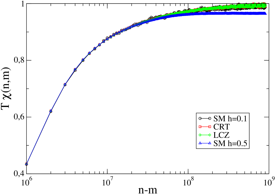
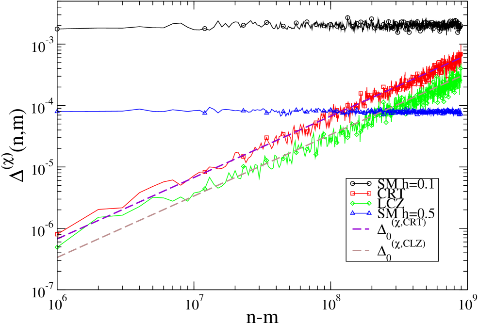
Figure 1: (Color online). Integrated auto-response function $\chi(n,m)$ (left panel) and its variance (right panel) in the 3-dimensional Ising model quenched from $T=\infty$ to $T_{c}=4.5115$. Left panel: Different curves correspond to computations performed with the SM (using two different values of $h$) and with the field-free algorithms of CRT and LCZ, as indicated in the key. In the right panel the behavior of the variances of the response function computed with the different methods is shown (continuous lines with heavy symbols, see key). The terms $\Delta^{(\chi,CRT)}_{0}$ and $\Delta^{(\chi,LCZ)}_{0}$ are also plotted (dashed lines).

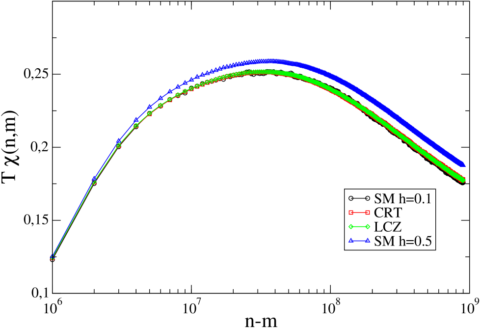
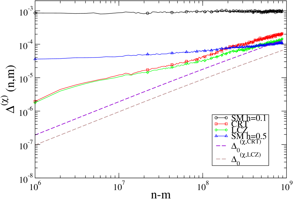
Figure 2: (Color online). As in Figure 1 for the 3-dimensional Ising model quenched from infinite temperature to $T=3<T_{c}$. Left Panel: Different algorithms yield the same result except the SM with the largest value of $h$ which, is always affected by non-linear effects.

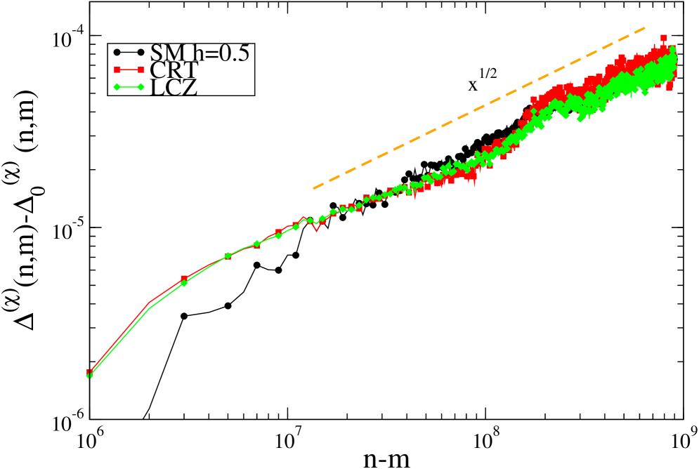
Figure 3: (Color online). Difference $\Delta^{(\chi)}(n,m)-\Delta^{(\chi)}_{0}(n,m)$ for the three algorithms in the Ising model quenched to $T=3$. The dashed orange line has slope 0.5.

In Fig. 4 we show the integrated response function and its variance in the EA model quenched to $T_{c}$ (left) and below $T_{c}$ (right). Here we take for $T_{c}$ the value obtained in ref. (eatc ). All the methods yield the same result except the SM with the largest value of $h$ which, for large values of $n-m$ ($n-m\gtrsim 6\cdot 10^{6}$ for $T=T_{c}$ (left) or $n-m\gtrsim 10^{7}$ for $T=1$ (right)) is affected by non-linear effects. The variances show the behavior similar to the one already discussed for the ferromagnetic Ising model. A notable difference is that, not only in the critical quench, but also in the sub-critical case, one has $\Delta^{(\chi)}\simeq\Delta^{(\chi)}_{0}$, indicating that $\Delta^{(\chi)}_{r}$ is always a sub-dominant contribution. We have explicitly checked that this happens also in quenches to lower temperatures ($T=0.5,T=0.2$). This possibly indicates that the argument developed above for ferromagnets cannot be straightforwardly extended to the low temperature phase of spin-glasses and that second order susceptibilities (or variances) may be used as efficient tools to characterize this difference.

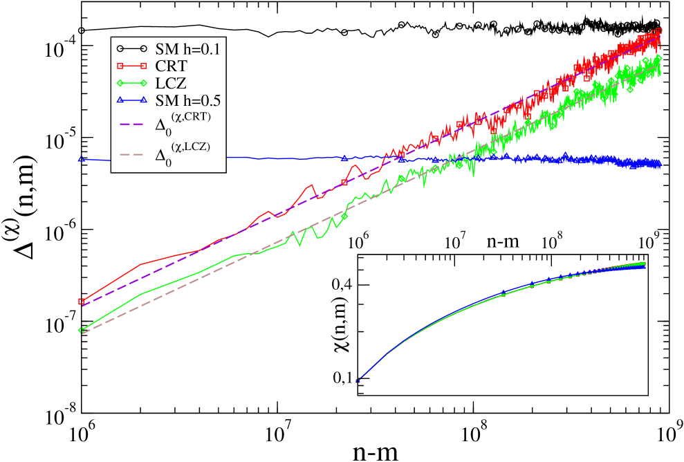
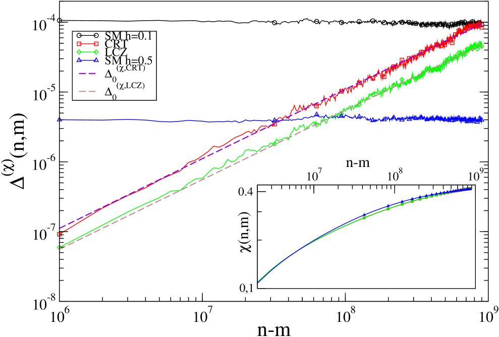
Figure 4: (Color online). The integrated auto-response function $\chi(n,m)$ (insets) and its variance (main) in the 3-dimensional EA model quenched from $T=\infty$ to $T_{c}\simeq 1.2$ (left panel) or to $T=1<T_{c}$. Insets: Different curves correspond to computations performed with the SM and two different values of $h$ and with the field-free algorithms of CRT and LCZ, as indicated in the key. In the main part of the two panels the behavior of the variances of the response computed with the different methods is shown (continuous lines with heavy symbols, see key). The terms $\Delta^{(\chi,CRT)}_{0}$ and $\Delta^{(\chi,LCZ)}_{0}$ are also plotted (dashed lines).

IV.2 Fredrickson-Andersen model

As stated in  lcz and discussed further in noi_nonlin ; noi_nonlin2 and in Sec. II of this Article, the FDR of LCZ can be derived in full generality in the context of Markovian dynamics, regardless of the model Hamiltonian and of the choice of transition probability. However, this claim has been questioned in mayersollich where the applicability of the LCZ algorithm to the FA model was doubted. However, the derivation of the LCZ relation as given above, or with different analytical techniques in Refs. noi_nonlin ; noi_nonlin2 ; baiesi , shows clearly its general character where no particular assumptions on the specific system nor on the form of the perturbation are made. In order to illustrate this issue also numerically, we have carried out the computation the integrated response function with the LCZ algorithm in the one-dimensional FA model.

The Hamiltonian of the FA model reads ${\cal H}(\sigma)=\sum_{i}\sigma_{i}$, where the $\sigma_{i}$ are bimodal variables taking the values ($0,1$), with $\sigma_{i}=1$ for a mobile fluid region and $\sigma_{i}=0$ an for an immobile one. Spins evolve according to transition probabilities obeying detailed balance, whose off-diagonal elements are

$$w_{i}(\sigma^{\prime}|\sigma)=[\epsilon(1-\sigma_{i})+(1-\epsilon)\sigma_{i}]\lambda_{i}(\sigma),$$ (70)

where $\epsilon=1/(1+e^{1/T})$ is the equilibrium density and $\lambda_{i}(\sigma)=\sigma_{i-1}+\sigma_{i+1}$ is a kinetic constraint that preserves detailed balance, due to the independence from $\sigma_{i}$. The integrated response function has been computed using both the SM and the LCZ algorithm. In the SM, the effect of the external field amounts to replace $\epsilon$ with $\epsilon_{i}^{h}=1/(1+e^{(1-h_{i})/T})$, whereas the quantity $B_{i}$ defined in Eq. (30) and entering the LCZ relation is given by

$$B_{i}(\sigma)=[\epsilon(1-\sigma_{i})+(1-\epsilon)\sigma_{i}]\lambda_{i}(\sigma)[1-2\sigma_{i}].$$ (71)

In Fig. 5 the comparison between the data obtained with the two methods and for three different temperatures, is presented. The value of $h$ used with the SM was checked to be in the linear regime. In particular we found that keeping the ratio $h/T=0.01$ constant satisfies the linearity requirement. The agreement between the two computations is excellent in the whole time range and for all the temperatures considered. Data for $T=1$ converge to the equilibrium value whereas results for $T=0.5$ and $T=0.2$ exhibit a non-monotonic behavior already observed in one-dimensional kinetic constrained models Crisanti2 . At low temperatures the equilibrium value is reached only asymptotically.

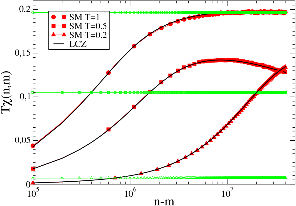
Figure 5: (Color online). Results of the numerical computation of the integrated auto-response function $\chi(n,m)$ for the one-dimensional FA model with $m=10^{5}$. The response functions computed with the SM (red filled symbols) and with the LCZ algorithm (continuous black lines), agree for the three temperatures. In the SM the external field is $h=0.01T$, satisfying linearity. The equilibrium value (green empty symbols) is also plotted for each temperature.

V Conclusions and perspectives

In this paper we have compared the FDR derived in a series of papers by CRT chatelain ; rt and LCZ lcz . First, by re-deriving them in a unified formalism we have pointed out that the distinction between these FDR is due to a different choice of the perturbed transition probabilities. Actually, even restricting to systems where detailed balance is obeyed, for a given choice of unperturbed transition probabilities an arbitrarity remains on the form of the perturbed ones, which is parametrized by the function $m_{j}$ defined in Eq. (10). In the case of Ising spins, selecting the value of $m_{j}$ corresponding to heat bath transition probabilities leads to the CRT relation (24). This FDR relates $R_{i,j}$ to a correlation function involving a $\delta$-function which weights only a subset of the whole ensemble of unperturbed trajectories. For this reason, the FDR of CRT, besides being limited to Ising spins with heat bath transition probabilities, can only be used in numerical simulations. On the other hand, making the choice $m_{j}=0$ of LCZ allows a further mathematical treatment leading to the FDR (29) where the response function is related to standard unperturbed correlations. This makes this relation basically different from those obtained in Berthier (Eq. (16) and in other approaches (i.e. in Crisanti ; Diez ), where the response function cannot be expressed in terms of correlations of observables. This makes the applicability of the LCZ relation in principle not restricted to simulations. Furthermore, this FDR has a larger degree of applicability with respect to the CRT, since it is not restricted to Ising spins nor to heat bath unperturbed transition probabilities.

In the second part of this Article, we have studied the efficiency of the CRT and LCZ field-free methods. In order to do that, we evaluate analytically the variances of the response function obtained with the SM or with the field-free methods. It turns out that, as far as the autoresponse function is considered, field-free methods are by far more efficient than the SM. This combines with the advantage of having linearity ($h\to 0$) built in. Moreover, we found that the LCZ algorithm is slightly more efficient (by a factor $\sqrt{2}$) than the method of CRT.

We conclude by pointing out that the results contained in this paper are not restricted to the framework of the efficient computation of the response function. Indeed, we mention that the study of the variances is closely connected to the issue of characterizing the fluctuation of two-time quantities in aging systems, a problem which has received a good deal of attention recently c4 . Moreover, as discussed at the end of Sec. III, the variance of the response function is also related to the second order susceptibility introduced in huse ; noi_nonlin ; noi_nonlin2 for the study of cooperativity.

VI Appendix I

We first prove Eq.(46)

$$1-\langle\sigma_{i}(m+1)\sigma_{i}(m)\rangle=\frac{1}{N}\left[1-\langle\sigma_{i}^{W}(m)\sigma_{i}(m)\rangle\right].$$ (72)

To do that, we first observe that from Eq.(3)

$$\langle 1-\sigma_{i}(m+1)\sigma_{i}(m)\rangle=\frac{1}{N}\sum_{\sigma^{\prime\prime},\sigma^{\prime}}[1-\sigma_{i}^{\prime\prime}\sigma_{i}^{\prime}]w_{i}\left(\sigma^{\prime\prime}|\sigma^{\prime}\right)P(\sigma^{\prime},m).$$ (73)

Only the term $w_{i}\left(\sigma^{\prime\prime}|\sigma^{\prime}\right)$ in the transition probability between the time $m$ and $m+1$ contributes. Hence the two configurations $\sigma^{\prime\prime}$ and $\sigma^{\prime}$ differ only for the spin on the $i-th$ site and sum on $\sigma^{\prime\prime}$ reduces to the sum on the two possible values $\pm\sigma_{i}^{\prime}$. Then, using the Heath bath form for the transition probabilities,

$$w_{j}\left(\sigma^{\prime\prime}|\sigma^{\prime}\right)=\frac{1}{2}\left(1+\sigma_{j}^{\prime\prime}\sigma_{j}^{W}(\sigma^{\prime})\right)$$ (74)

one obtains Eq.(72).

Next we prove Eq.(48). Let us first proof that

$$\langle[\sigma_{j}(m+1)-\sigma^{W}_{j}(m)]\sigma^{W}_{j}(m)\delta_{I(m),j}\rangle=0.$$ (75)

From the definition one has

$$\langle\left[\sigma_{j}(m+1)-\sigma_{j}^{W}(m)\right]\sigma_{i}^{W}(m)\delta_{I(m),j}\rangle=\sum_{\sigma^{\prime\prime},\sigma^{\prime}}\left[\sigma_{j}^{\prime\prime}-\sigma_{j}^{W}(\sigma^{\prime})\right]w_{j}\left(\sigma^{\prime\prime}|\sigma^{\prime}\right)\delta_{I(m),j}P(\sigma^{\prime},m).$$ (76)

Because of the delta function, one has that the configurations $\sigma^{\prime}$ and $\sigma^{\prime\prime}$ can differ only for the spin in the $j$-th site. This implies that $\sigma_{j}^{W}(\sigma^{\prime})=\sigma_{j}^{W}(\sigma^{\prime\prime})$ and that the sum on $\sigma^{\prime\prime}$ reduces to the sum on the two possible values $\pm\sigma_{j}^{\prime}$. The Heath-Bath form (74) for the $w$ then gives

$$\sum_{\sigma_{j}^{\prime\prime}=\pm\sigma_{j}^{\prime}}\left[\sigma_{j}^{\prime\prime}-\sigma_{j}^{W}(\sigma^{\prime})\right]w_{j}\left(\sigma^{\prime\prime}|\sigma^{\prime}\right)=0,$$ (77)

which implies Eq.(75). We next observe that from Eq.(20)

$$\langle\sigma_{j}^{W}(m)^{2}\delta_{I(m),j}\rangle=\frac{1}{N}\sum_{I(m)}\sum_{\sigma^{\prime},\sigma}(\sigma_{j}^{W})^{2}w(\sigma^{\prime}|\sigma)P(\sigma,m)\delta_{I(m),j}=\frac{1}{N}\langle\sigma_{j}^{W}(m)^{2}\rangle.$$ (78)

Combining the above result with Eq.(75) one recovers Eq.(48).

VII Appendix II

Here we prove that $R^{(2)}_{i,j}(n,m,m^{\prime})=\langle r_{i,j}(n,m)r_{i,j}(n,m^{\prime})\rangle$ is identically zero for all the algorithms if $m\neq m^{\prime}$.

1. Standard method

   In the SM one applies a random magnetic field $h_{i}$, with $\overline{h}_{i}=0$ and $\overline{h_{i}h_{j}}=\delta_{ij}$, and the response is obtained as

   $$R_{i,j}(n,m)=N\overline{\frac{\langle\sigma_{i}(n)h_{j}\delta_{I(m),j}\rangle}{h^{2}}}.$$ (79)

   Therefore

   $$R^{(2)}_{i,j}(n,m,m^{\prime})=\frac{N}{h^{2}}\delta_{m,m^{\prime}}$$ (80)

2. CRT relation

   In this case $r_{i,j}$ can be directly read off from Eq. (21). From Eq. (15) one has

   $$\sum_{\sigma^{\prime\prime},\sigma^{\prime}}w_{i}(\sigma^{\prime\prime}|\sigma^{\prime})f_{i}(\sigma^{\prime\prime},\sigma^{\prime})[1-\delta_{\sigma^{\prime\prime},\sigma^{\prime}}]P(\sigma^{\prime},m|\sigma,m^{\prime})=-\sum_{\sigma^{\prime}}w_{i}(\sigma^{\prime}|\sigma^{\prime})g_{i}(\sigma^{\prime})\delta_{\sigma^{\prime\prime},\sigma^{\prime}}P(\sigma^{\prime},m|\sigma,m^{\prime})$$ (81)

   that gives

   $$\langle f_{i}(m)O(m^{\prime})\rangle_{flip}+\langle g_{i}(m)O(m^{\prime})\rangle_{noflip}=0,$$ (82)

   for every generic observable $O$ computed at the shorter time $m^{\prime}$. Therefore,

   $$R^{(2)}_{i,j}(n,m,m^{\prime})=0$$ (83)

   for $m^{\prime}\leq m-1$.

3. LCZ relation

   Reading $r_{i,j}$ from Eq. (29), using the property (31) one obtains that $\langle[\Delta\sigma_{i}(m)-B_{i}(m)]O(m^{\prime})\rangle=0$, for every generic observable $O$ computed at the shorter time $m^{\prime}$. Therefore one arrives again at Eq. (83) for $m^{\prime}\leq m-1$.

VIII Appendix III: Numerical impementation of alghorithms for the computation of integrated response functions

1. Standard method

   For each realization of the dynamical trajectory, a random magnetic field $h_{i}$ is assigned to each site. $h_{i}$ is usually chosen from a bimodal distribution $h_{i}=\pm h$. The evolution is then controlled by unperturbed transition probabilities until the time $m$ and by the perturbed ones given in Eq.(8) for later times. At the time $n$, the integrated response function is computed according to Eq.(57).

2. CRT relation

   The integrated response function can be obtained from the space and time integral of Eq. (24)

   $$\chi^{(CRT)}(n,m)=\frac{\beta}{N}\sum_{i}\langle\sigma_{i}(n)\Lambda_{i}(n,m),\rangle$$ (84)

   with

   $$\Lambda_{i}(n,m)=\sum_{l=m}^{n-1}\left[\sigma_{i}(l+1)-\sigma_{i}^{W}(l)\right].$$ (85)

   In each realization of the dynamics, the quantity $\Lambda_{i}$ is initially set to zero on each site. For all the timesteps $l\geq m$, $\Lambda_{j}$ is updated, via the relation

   $$\Lambda_{j}=\Lambda_{j}+\sigma_{i}(l+1)-\sigma_{i}^{W}(l),$$ (86)

   only on the site $j=I(l)$ where the flip of the spin has been attempted. Elsewhere $\Lambda_{i}$ is left unchanged. At each time $n\geq m$, $\chi(n,m)$ is then computed according to Eq.(84).

3. LCZ relation

   From Eq. (29) one immediately obtains

   $$\chi^{(LCZ)}(n,m)=\frac{\beta}{2N}\sum_{i}\left[\langle\sigma_{i}(n)\sigma_{i}(n)\rangle-\langle\sigma_{i}(n)\sigma_{i}(m)\rangle+\langle\sigma_{i}(n-1)A_{i}(n,m)\rangle\right]$$ (87)

   with

   $$A_{i}(n,m)=\frac{1}{N}\sum_{l=m}^{n-1}B_{i}(l).$$ (88)

   The quantity $\langle\sigma_{i}(n)\sigma_{i}(m)\rangle$ is the usual two time correlations function. Concerning the evaluation of $A_{i}$, the basic observation is that, according to Eq.(68), $B_{i}$ only depends on the spin $\sigma_{i}$ and on the spins interacting with it. In particular, for the models considered in this paper, $B_{i}$ depends on $\sigma_{i}$ and on its nearest-neighboring spins. The evaluation of $A_{i}$ proceeds as follows. At the time $m$, $B_{i}$ is evaluated on each site according to Eq.(68), $A_{i}$ is set to zero and $l_{i}$ is set to $m$. $l_{i}$ represents the time where the last evaluation of $B_{i}$ has been performed. $B_{i}$ is then left unchanged on all sites until a spin flip occurs. If the spin flip occurs on site $I(l)$ at time $l$, $A_{j}$ is updated as

   $$A_{I(l)}=A_{I(l)}+B_{I(l)}(l_{j})\left(l-l_{j}\right)/N.$$ (89)

   $l_{j}$ is then set to $l$ and the new value of $B_{j}$ is evaluated. The same procedure is repeated for all the spins interacting with $\sigma_{I(l)}$, leaving unchanged $A_{i}$, $B_{i}$ elsewhere. In the end $A_{i}(n,m)$ is obtained via the relation

   $$A_{i}(n,m)=A_{i}+B_{i}(l_{i})\left(n-l_{i}\right)/N,$$ (90)

   and the integrated response function is computed according to Eq.(87).

References

- (1) L.F. Cugliandolo, J. Kurchan and L. Peliti, Phys. Rev. E 55 3898 (1997).
- (2) S. Franz, M. Mézard, G. Parisi and L. Peliti , Phys. Rev. Lett. 81 1758 (1998); J. Stat. Phys. 97 459 (1999).
- (3) C. Donati, S.C. Glotzer and P. Poole, Phys. Rev. Lett. 82, 5064 (1999); S. Franz, C. Donati, G. Parisi and S.C. Glotzer, Phil.Mag.B 79, 1827 (1999); S. Franz and G. Parisi, J. Phys.: Condens.Mat. 12, 6335 (2000); A. Annibale and P. Sollich, J. Stat. Mech. P02064 (2009); F. Corberi and L.F. Cugliandolo, J. Stat. Mech. P05010 (2009); C. Chamon and L. F. Cugliandolo, J. Stat. Mech. P07022 (2007); C. Chamon, L.F. Cugliandolo, and H. Yoshino, J. Stat. Mech. P01006 (2006); C. Chamon, P. Charbonneau, L. F. Cugliandolo, D. R. Reichman, M. Sellitto, J. Chem. Phys. 121, 10120 (2004); H.E. Castillo, C. Chamon, L.F. Cugliandolo, J.L. Iguain, and M.P. Kennett, Phys. Rev. B 68, 134442 (2003).
- (4) L.F. Cugliandolo, J. Kurchan and G.Parisi, J. Phys.I France 4, 1641 (1994).
- (5) A. Crisanti and F. Ritort, J. Phys. A 36, R181 (2003).
- (6) C.Chatelain, J. Phys. A 36, 10739 (2003).
- (7) F. Ricci-Tersenghi, Phys. Rev.E 68, 065104(R) (2003).
- (8) E. Lippiello, F. Corberi and M. Zannetti, Phys. Rev. E 71, 036104 (2005).
- (9) G. Diezemann, Phys. Rev. E 72, 011104 (2005).
- (10) L. Berthier, Phys. Rev. Lett. 98, 220601 (2007).
- (11) E. Lippiello, F. Corberi, A. Sarracino and M. Zannetti, Phys. Rev. B 77, 212201 (2008).
- (12) E. Lippiello, F. Corberi, A. Sarracino and M. Zannetti, Phys. Rev. E 78, 041120 (2008).
- (13) J.P.Bouchaud and G.Biroli, Phys. Rev.B 72, 064204 (2005).
- (14) P. Mayer and P. Sollich, J. Phys. A 40, 5823 (2007).
- (15) F. Corberi, E. Lippiello, and Marco Zannetti, Phys. Rev. E 72, 056103 (2005); Phys. Rev. E 74, 041106 (2006); E. Lippiello, F. Corberi and Marco Zannetti, Phys. Rev. E 74, 041113 (2006); N. Andrenacci, F. Corberi and E. Lippiello, Phys. Rev. E 74, 031111 (2006); R. Burioni, D. Cassi, F. Corberi, and A. Vezzani, Phys. Rev. Lett. 96, 235701 (2006); Phys. Rev. E 75, 011113 (2007); F. Corberi, A. Gambassi, E. Lippiello, and Marco Zannetti, J. Stat. Mech. P02013 (2008); F.Corberi and L.F.Cugliandolo, J. Stat. Mech. P05010 (2009); J. Stat. Mech. P09015 (2009).
- (16) N. Andrenacci, F. Corberi and E. Lippiello, Phys. Rev. E 73 046124 (2006).
- (17) A. Barrat, Phys. Rev. E 57 (1998) 3629; L. Berthier, J.L. Barrat and J. Kurchan, Eur. Phys. J. B 11, (1999); F. Corberi, E. Lippiello, and M. Zannetti, Phys. Rev. E 63, 061506 (2001); Eur. Phys. J. B 24 (2001), 359; Phys.Rev. E 68, 046131 (2003).
- (18) D.A. Huse, J. Appl. Phys. 64, 5776 (1988).
- (19) F. Corberi, E. Lippiello and M. Zannetti, J. Stat. Mech. P12007 (2004).
- (20) A. Ogielski and I. Morgenstern, Phys. Rev. Lett. 54, 928 (1985); H.G. Katzgraber, M. Korner and A.P. Young, Phys. Rev. B 73, 224432 (2006), and references therein.
- (21) M. Baiesi, C. Maes, and B. Wynants, Phys. Rev. Lett. 103, 010602 (2009).
- (22) A. Crisanti, F. Ritort, A. Rocco and M. Sellitto, J. Chem. Phys. 113, 10615 (2000).