Diagrammatic analysis of the Hubbard model:
Stationary property of the thermodynamic potential

Abstract

Diagrammatic approach proposed many years ago for strong correlated Hubbard model is developed for analyzing of the thermodynamic potential properties. The new exact relation between such renormalized quantities as thermodynamic potential, one-particle propagator and correlation function is established. This relation contains additional integration of the one-particle propagator by the auxiliary constant. The vacuum skeleton diagrams constructed from irreducible Green’s functions and tunneling propagator lines are determined and special functional is introduced. The properties of such functional are investigated and its relation to the thermodynamic potential is established. The stationary properties of this functional with respect to first order changing of the correlation function is demonstrated and as a consequence the stationary properties of the thermodynamic potential is proved.

I Introduction

The Hubbard model is one of the most important models for the electron of solids which describes quantum mechanical hopping of electron between lattice sites and their short ranged repulsive Coulomb interaction.

This model was discussed by Hubbard ^[1] in order to describe a narrow-band system of transition metals and has been revised to investigate the properties of highly correlated electron systems such as the copper oxide superconductors and others.

Hubbard model exhibits various phenomena including metal-insulator transition, antiferromagnetism, ferromagnetism and superconductivity. This model assumes that each atom of the crystal lattice has only one electron orbit and the corresponding orbital state is non degenerate.

The Hamiltonian of Hubbard model is a sum of the two terms

$$H = H^{0}+H^{\prime},$$ (1)

where $H^{0}$ is the atomic contribution, which contains the Coulomb interaction term $U$ and local electron energy $\overline{\epsilon}$ on the atom

$$H^{0} = \sum\limits_{\overrightarrow{i}}H_{\overrightarrow{i}}^{0},$$

$$H_{\overrightarrow{i}}^{0} = \sum\limits_{\sigma}\epsilon n_{\overrightarrow{i}\sigma}+Un_{\overrightarrow{i}\uparrow}n_{\overrightarrow{i}\downarrow},$$ (2)

$$\epsilon = \overline{\epsilon}-\mu,\quad n_{\overrightarrow{i}\sigma}=C_{\overrightarrow{i}\sigma}^{+}C_{\overrightarrow{i}\sigma}$$

and hopping Hamiltonian

$$H^{\prime} = \sum\limits_{\overrightarrow{i}\overrightarrow{j}}\sum\limits_{\sigma}t(\overrightarrow{i}-\overrightarrow{j})C_{\overrightarrow{i}\sigma}^{+}C_{\overrightarrow{j}\sigma},$$ (3)

$$t(\overrightarrow{i}-\overrightarrow{j}) = t^{*}(\overrightarrow{j}-\overrightarrow{i}),\quad t(0)=0.$$

Here $C_{\overrightarrow{i}\sigma}^{+}(C_{\overrightarrow{i}\sigma})$ are the creation (annihilation) electron operators with local site $\overrightarrow{i}$ and spin $\sigma$. Because in the thermodynamic perturbation theory we shall use thermal averages in a grand canonical ensemble we have added to the Hamiltonian (1) the term $-\mu\hat{N}_{e}$

$$\hat{N}_{e} = \sum\limits_{\overrightarrow{i}\sigma}n_{\overrightarrow{i}\sigma}$$ (4)

where $\mu$ is the chemical potential and $\hat{N}_{e}$ electron number operator. The quantities $U$ and $\hat{N}_{e}$ are the fundamental parameters of the model and because of large value of the Coulomb repulsion it is taken into account in zero approximation of our theory. The operator $H^{\prime}$, which describes hopping of the electrons between sites of the crystal lattice is regarded as a perturbation.

For investigating this model new physical and mathematical concepts and techniques have been elaborated. We can only enumerate some of them. There are many analytical approximations as Hubbard approximation, noncrossing approximation (NCA), slave-boson method, Dynamical Mean Field Theory (DMFT), composite and others projection operator methods and approaches. Also numerical simulations of thermodynamic quantities and density of states have been performed by various methods. Some exact results for one- and two-dimensional Hubbard model are known. Each approximate method has its advantages and disadvantages. A short and comprehensive reviews of the methods can be found in papers and books ^[2-7]. Besides these approaches we must enumerate also the special diagram techniques elaborated for strongly correlated electron systems. Stasyuk ^[8], Zaitsev ^[9], Izyumov ^[10] and coworkers have developed a diagram technique for Hubbard model, based on the disentangling of nondiagonal Hubbard operator $\chi{mn}$ out of a time-ordered products of other such operators. Due to a more complicate algebra of Hubbard transfer operator than that for Fermi operators the essential features of this technique remain till now poorly developed.

The other diagrammatic approach around the atomic limit also has been proposed for Hubbard model both in normal ^[11,12] and in superconducting state ^[13]. This theory introduces the Generalized Wick Theorem (GWT) that uses cumulant expansion of the statistical average values for the products of the Fermion operators. The GWT takes into account the fact that Hamiltonian $H^{0}$ is nonquadratic in fermion operators due to Coulomb interaction. This last circumstance is responsible for the appearance of the nonvanishing site cumulants called irreducible Green’s functions. These new Green’s functions take into account all the spin, charge and pairing fluctuations of the system. The perturbation formalism around atomic limit has the advantage that local (atomic) physical properties can be evaluated exactly and that the transfer of this local information to neighboring sites due to the kinetic mobility of the conduction electrons can be handled perturbatively in powers of hopping integral.

A GWT for chronological averages of products of electron operators was formulated later also by Metzner ^[14]. Metzner did not derive a Dyson-type equation for the renormalized one-particle Green’s function and the role of our correlation function has not established.

In spite of the similarity to our works, the diagrams in his approach are quite different. The $n$ - particle cumulant is represented a $2n$ - valent-point vertex with attached $n$ entering and $n$ leaving lines, where as our such a cumulant or irreducible Green function is represented by a rectangle with $2n$ vertices with $n$ entering and $n$ leaving arrows. The rectangle contours the vertices with the same site index but different time and spin labels. In addition Metzner investigated the limit of high lattice dimensions.

In this paper we shall develop the diagrammatic theory proposed before for Hubbard model ^[11,12] with the aim to demonstrate the existence of the relation between renormalized quantities of thermodynamic potential and one-particle Green’s function and also to prove the stationary properties of this potential.

Such theorem was proved firstly by Luttinger and Ward ^[15] for uncorrelated systems by using the diagrammatic technique of weak coupling field theory.

The strong coupling diagram theory used by us needs new conceptions and new equations and they are used to prove stationary property of thermodynamic potential for strongly correlated systems. Such a proof has been already achieved for Anderson impurity model in paper ^[16].

The paper is organized in the following way. In section II we develop the diagrammatic theory in the strong coupling limit and the skeleton diagrams are introduced. In Section III we prove the stationary theorem for renormalized thermodynamic potential. Section IV has the conclusions.

II Perturbation Treatment

We shall use the definition of the one-particle Matsubara Green’s functions in interaction representation as in paper ^[11,12]:

$$G(x|x^{\prime}) = -\ \left\langle TC_{\overrightarrow{x}\sigma}(\tau)\overline{C}_{\overrightarrow{x}^{\prime}\sigma^{\prime}}(\tau^{\prime})U(\beta)\right\rangle_{0}^{c},$$ (5)

where $x$ stands for $(\overrightarrow{x},\sigma,\tau)$ and index $c$ for $\left\langle...\right\rangle_{0}^{c}$ means the connected part of the diagrams which appear in the right-hand of part of (5). We use the series expansion for the evolution operator $U(\beta)$ with some generalization because we introduce the auxiliary constant $\lambda$ and use $\lambda H^{\prime}$ instead of $H^{\prime}$:

$$U_{\lambda}(\beta) = T\exp(-\lambda\int\limits_{0}^{\beta}H^{\prime}(\tau)d\tau).$$ (6)

In the presence of this constant we shall use index $\lambda$ for all dynamical quantities as $G_{\lambda}(x|x^{\prime})$ and so on. At the last stage of the calculations this constant will be put equal to one.

In zero order approximation the one-particle Green’s function $G^{(0)}(x|x^{\prime})$ is local

$$G^{(0)}(x|x^{\prime}) = \delta_{\overrightarrow{x}\overrightarrow{x}^{\prime}}\delta_{\sigma\sigma{\prime}}G^{(0)}(\tau-\tau^{\prime})$$ (7)

and the Fourier representation of the last function is

$$G_{\sigma}^{(0)}(i\omega_{n}) = \int\limits_{0}^{\beta}G_{\sigma}^{(0)}(\tau)e^{i\omega_{n}\tau}d\tau$$

$$= \frac{1}{Z_{0}}\{\frac{e^{-\beta E_{0}}+e^{-\beta E_{\sigma}}}{i\omega_{n}+E_{0}-E_{\sigma}}+\frac{e^{-\beta E_{\overline{\sigma}}}+e^{-\beta E_{2}}}{i\omega_{n}+E_{\overline{\sigma}}-E_{2}}\},$$

$$Z_{0} = e^{-\beta E_{0}}+e^{-\beta E_{\sigma}}+e^{-\beta E_{\overline{\sigma}}}+e^{-\beta E_{2}},$$

$$E_{0} = 0,\quad E_{\sigma}=E_{\overline{\sigma}}=\epsilon,\quad E_{2}=2\epsilon+U,$$

$$\omega_{n} = (2n+1)\pi/\beta.$$

Here $E_{0},E_{\sigma}$ and $E_{2}$ are the energies of atomic sites.

As has been proved in papers ^[11,12] propagator (5) has the diagrammatic representation depicted on the Fig. 1.

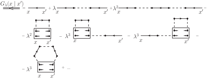
Figure 1: First three orders of perturbation theory for one-particle propagator. The thin solid line depicts zero order propagator, thin dashed line depicts the tunneling matrix element. The rectangles depict irreducible two-particles Green’s functions $G_{2}^{(0)ir}$ and points are the vertices of diagrams.

The irreducible Green’s functions of order $n$ are depicted with rectangles with $2n$ vertices. The arrows which enter in the vertex point depict annihilation electrons and that which go out the created electrons.

In paper ^[11] we have introduced the notion of correlation function $Z_{\lambda}(x|x^{\prime})$ which is the sum of strongly connected diagrams containing irreducible Green’s functions and related to a more convenient function $\Lambda_{\lambda}(x|x^{\prime})=G^{0}(x|x^{\prime})+Z_{\lambda}(x|x^{\prime})$.

In Fig. 1 the fourth and seventh diagrams of the right-hand site belong to correlation function. Due to the fact that irreducible functions are local and tunneling matrix elements have the property $t(\overrightarrow{x}-\overrightarrow{x})=0$ in Fig. 1 are omitted all the diagrams which contain self-locked tunneling elements.

As is seen from Fig. 1 the process of propagator renormalization is accompanied by the analogous process for tunneling matrix elements renormalization and replacing of the instant quantity $\lambda t(x-x^{\prime})=\lambda t(\overrightarrow{x}-\overrightarrow{x}^{\prime})\delta(\tau-\tau^{\prime}-0^{+}))$ by dynamical one $\widetilde{T}_{\lambda}(x|x^{\prime})$ equal to

$$\widetilde{T}_{\lambda}(x|x^{\prime}) = \lambda t(\overrightarrow{x}-\overrightarrow{x}^{\prime})\delta(\tau-\tau^{\prime}-0^{+})$$ (9)

$$+ \sum\limits_{12}\lambda t(x-1)G_{\lambda}(1|2)\lambda t(2-x^{\prime})$$

which in Fourier representation

$$t(\overrightarrow{x}) = \frac{1}{N}\sum\limits_{\overrightarrow{k}}\epsilon(\overrightarrow{k})\exp{(-i\overrightarrow{k}\overrightarrow{x})},$$

$$G_{\lambda}(x|x^{\prime}) = \frac{1}{N}\sum\limits_{\overrightarrow{k}}\frac{1}{\beta}\sum\limits_{\omega_{n}}G_{\lambda}(\overrightarrow{k}|i\omega_{n})$$

$$\times \exp{[-i\overrightarrow{k}(\overrightarrow{x}-\overrightarrow{x}^{\prime})-i\omega_{n}(\tau-\tau^{\prime})]}$$

has a form:

$$\widetilde{T}_{\lambda}(\overrightarrow{k}|i\omega_{n}) \equiv \lambda T_{\lambda}(\overrightarrow{k}|i\omega_{n})$$ (10)

$$= \lambda\epsilon(\overrightarrow{k})(1+\lambda\epsilon(\overrightarrow{k})G_{\lambda}(\overrightarrow{k}|i\omega_{n}))$$

The renormalized tunneling matrix element $T_{\lambda}$ really is tunneling Green’s function and will be depicted as double dashed line. $\widetilde{T}_{\lambda}$ is represented by such double dashed line multiplied by $\lambda$.

Now we introduce the skeleton diagrams which contain only irreducible Green’s functions and simple dashed lines without any renormalization. In such skeleton diagrams the thin dashed lines are replaced by double dashed lines with realizing the complete renormalization of dynamical quantities.

The skeleton diagrams for correlation $\Lambda_{\lambda}$ function are depicted on Fig. 2.

As can bee seen from Fig. 2 the skeleton diagrams for $\Lambda(k)$ function are of two kinds. The first four diagrams of this Figure are local and therefore their Fourier representation don’t depend on momentum. The last diagram and other ones with more number of rectangles are non localized and their Fourier representation depends on momentum. Only the first category of diagram are taken into account in Dynamical Mean Field Theory.

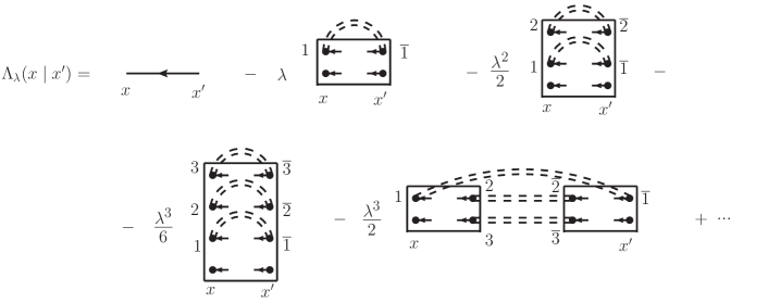
Figure 2: The skeleton diagrams for correlation function $\Lambda_{\lambda}$. Double dashed lines depict the tunneling Green’s functions $T_{\lambda}$ and the rectangles depict the irreducible Green’s functions.

As was proved in papers ^[11,12] the knowledge of this function permits to formulate the following Dyson-type equation for one-particle Green’s function

$$G_{\lambda}(k)=\frac{\Lambda_{\lambda}(k)}{1-\lambda\epsilon(\overrightarrow{k})\Lambda_{\lambda}(k)}.$$ (11)

Here $k$ stands for $(\overrightarrow{k},i\omega_{n})$ with odd Matsubara frequencies. Equation (10) and (11) gives us the results

$$\widetilde{T}_{\lambda}(k) = \lambda T_{\lambda}(k),$$

$$T_{\lambda}(k) = \frac{\epsilon(\overrightarrow{k})}{1-\lambda\epsilon(\overrightarrow{k})\Lambda_{\lambda}(k)}.$$ (12)

Equation (12) has a form of Dyson equation for tunnelind Green’s function, and the role of mass operator $\Sigma_{\lambda}$ is carried out by correlation function multiplied by auxiliary constant $\lambda$:

$$\Sigma_{\lambda}(k) = \lambda\Lambda_{\lambda}(k).$$ (13)

In Hubbard I approximation we neglect the correlation function $Z_{\lambda}(k)$ and consider function $\Lambda_{\lambda}(k)$ equal to zero order Green’s function $G^{0}(k)$. In this approximation we have

$$G_{\lambda}^{I}(k)=\frac{G^{0}(k)}{1-\lambda\epsilon(\bf{k})G^{0}(k)},$$

which describes two Hubbard energy subbands distanced between them for $U\neq 0$ and without the possibility to describe the Mott-Hubbard transition.

III Thermodynamic potential diagrams

The thermodynamic potential of the system is determined by the connected part of the mean value of the evolution operator ^[11,12]

$$F = F_{0}-\frac{1}{\beta}\left\langle U(\beta)\right\rangle_{0}^{c}.$$ (14)

Let us consider a more general quantity first

$$F(\lambda) = F_{0}-\frac{1}{\beta}\left\langle U_{\lambda}(\beta)\right\rangle_{0}^{c},$$ (15)

and put then $\lambda=1$.

By using the perturbation theory we have obtained the first orders of diagrams for $\left\langle U_{\lambda}(\beta)\right\rangle_{0}^{c}$, depicted in Fig. 3.

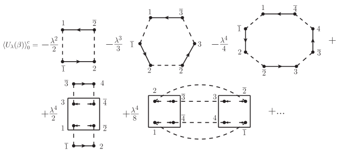
Figure 3: The first four orders of perturbation theory for $\left\langle U_{\lambda}(\beta)\right\rangle_{0}^{c}$.

In order to obtain the better understanding of these diagrammatic contributions we examine the expression

$$\sum\limits_{xx^{\prime}}G_{\lambda}(x|x^{\prime})\lambda t(\overrightarrow{x}^{\prime}-\overrightarrow{x})\delta(\tau-\tau^{\prime}-0^{+})\delta_{\sigma\sigma^{\prime}},$$ (16)

where double repeated indices suppose summation and integration. Consequently (16) is equal to

$$- \beta\sum\limits_{\overrightarrow{x}\overrightarrow{x}^{\prime}}\sum\limits_{\sigma}G_{\lambda\sigma}(\overrightarrow{x}-\overrightarrow{x}^{\prime}|-0^{+})\lambda t(\overrightarrow{x}^{\prime}-\overrightarrow{x})$$ (17)

$$= -\lambda\sum\limits_{\overrightarrow{k}\sigma}\sum\limits_{\omega_{n}}\epsilon(\overrightarrow{k})G_{\lambda\sigma}(\overrightarrow{k}|i\omega_{n})\exp(i\omega_{n}0^{+}).$$

Here we have carried out the integration by time.

From diagrammatic point of view equation (16) implies the procedure of locking of the external lines of propagators $G_{\lambda}$ diagrams depicted on the Fig. 1 with the tunneling matrix element $t(\overrightarrow{x}^{\prime}-\overrightarrow{x})$ and obtaining in such a way the diagrams without external lines similar with ones for $\left\langle U_{\lambda}(\beta)\right\rangle_{0}^{c}$ depicted on Fig. 3. These two series of diagrams differ by coefficients in front of them.

In expression (17) the coefficients $\frac{1}{n}$ before each diagram are absent, where $n$ is the order of perturbation theory. These coefficients are present in Fig. 3. In order to restore these $\frac{1}{n}$ coefficients in (17) and obtain the coincidence with $\left\langle U_{\lambda}(\beta)\right\rangle_{0}^{c}$ series it is enough to integrate by $\lambda$ the expression (17) and obtain:

$$-\sum\limits_{\overrightarrow{x}\overrightarrow{x}^{\prime}}\sum\limits_{\sigma}\beta\int d\lambda t(\overrightarrow{x}^{\prime}-\overrightarrow{x})G_{\lambda\sigma}(\overrightarrow{x}-\overrightarrow{x}^{\prime}|-0^{+}).$$ (18)

The expression (18) displayed in a diagrammatic representation coincides exactly with mean value of the evolution operator:

$$\left\langle U_{\lambda}(\beta)\right\rangle_{0}^{c} = -\sum\limits_{\overrightarrow{x}\overrightarrow{x}^{\prime}}\beta t(\overrightarrow{x}^{\prime}-\overrightarrow{x})$$ (19)

$$\times \int\limits_{0}^{\lambda}d\lambda^{\prime}G_{\lambda^{\prime}\sigma}(\overrightarrow{x}-\overrightarrow{x}^{\prime}|-0^{+}).$$

In Fourier representation we have

$$\left\langle U_{\lambda}(\beta)\right\rangle_{0}^{c}=-\int\limits_{0}^{\lambda}d\lambda^{\prime}\sum\limits_{\overrightarrow{k}\sigma\omega_{n}}\epsilon(\overrightarrow{k})G_{\lambda^{\prime}\sigma}(\overrightarrow{k}|i\omega_{n})\exp(i\omega_{n}0^{+}).$$

(20)

From (15) and (20) we obtain

$$F(\lambda) = F_{0}+\int\limits_{0}^{\lambda}d\lambda^{\prime}\sum\limits_{\overrightarrow{k}\sigma}\frac{1}{\beta}\sum\limits_{\omega_{n}}\epsilon(\overrightarrow{k})$$ (21)

$$\times G_{\lambda^{\prime}\sigma}(\overrightarrow{k}|i\omega_{n})\exp(i\omega_{n}0^{+}).$$

Using the definition (14), the equation (21) can be written in the form:

$$F(\lambda) = F_{0}+\int\limits_{0}^{\lambda}\frac{d\lambda^{\prime}}{\lambda^{\prime}}\sum\limits_{\overrightarrow{k}\sigma}\frac{1}{\beta}\sum\limits_{\omega_{n}}T_{\lambda^{\prime}}(k)$$ (22)

$$\times \Sigma_{\lambda^{\prime}}(k)\exp(i\omega_{n}0^{+}).$$

From (22) we have

$$\lambda\frac{F(\lambda)}{d\lambda} = \sum\limits_{\overrightarrow{k}\sigma}\frac{1}{\beta}\sum\limits_{\omega_{n}}T_{\lambda}(k)\Sigma_{\lambda}(k)\exp(i\omega_{n}0^{+})$$ (23)

$$= \frac{1}{\beta}Tr(T_{\lambda}\Sigma_{\lambda}).$$

In order to have a full system of equations we add to (22) the definition of the chemical potential of the system

$$N_{e} =\sum\limits_{\overrightarrow{k}\sigma}\frac{1}{\beta}\sum\limits_{\omega_{n}}G_{\sigma}(\overrightarrow{k}|i\omega_{n})\exp(i\omega_{n}0^{+}),$$ (24)

where $N_{e}$ is the electron number.

Equation (21) establishes the relation between thermodynamic potential and renormalized one-particle propagator. This last quantity depends on the auxiliary parameter $\lambda$ and (21) contains an additional integration over it and is awkward because that.

We shall obtain more convenient equation for thermodynamic potential without such integration by $\lambda$. For that we shall introduce a special functional

$$Y(\lambda)=Y_{1}(\lambda)+Y^{\prime}(\lambda),$$ (25)

where

$$Y_{1}(\lambda) = -\frac{1}{\beta}\sum\limits_{\overrightarrow{k},\sigma,\omega_{n}}[\ln(\epsilon(\overrightarrow{k})\lambda\Lambda_{\lambda}(k)-1)$$ (26)

$$+ T_{\lambda}(k)\lambda\Lambda_{\lambda}(k)]\exp(i\omega_{n}0^{+}),$$

and $Y^{\prime}(\lambda)$ is constructed from skeleton diagrams without external lines and is depicted on Fig.4

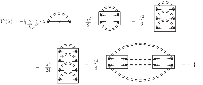
Figure 4: The simplest skeleton diagrams for functional $Y^{\prime}(\lambda)$. Double dashed lines are tunneling functions $T_{\lambda}(k)$.

The dependence on $\lambda$ in the functional $Y^{\prime}(\lambda)$ is twofold, just through the dependence of the renormalized Green’s functions $G_{\lambda},T_{\lambda},\Lambda_{\lambda}$ and $\Sigma_{\lambda}$ and through the explicit factors $\lambda^{n}$ in front of each diagram of $Y^{\prime}(\lambda)$.

By using these definitions we can prove the equations

$$\frac{\delta\beta Y_{1}(\lambda)}{\delta T_{\lambda}(k)} = -\lambda\Lambda_{\lambda}(k)=-\Sigma_{\lambda}(k),$$

$$\frac{\delta\beta Y^{\prime}(\lambda)}{\delta T_{\lambda}(k)} = \lambda\Lambda_{\lambda}(k)=\Sigma_{\lambda}(k),$$ (27)

and as a result we obtain the stationary property:

$$\frac{\delta\beta Y(\lambda)}{\delta T_{\lambda}(k)}=0.$$ (28)

By using the definition (13) of the mass operator $\Sigma_{\lambda}(k)$ we can rewrite the functional $Y_{1}(\lambda)$ in the form

$$Y_{1}(\lambda) = -\frac{1}{\beta}\sum\limits_{\overrightarrow{k}\sigma}\sum\limits_{\omega_{n}}[\ln(\epsilon(\overrightarrow{k})\Sigma_{\lambda}(k)-1)$$ (29)

$$+ T_{\lambda}(k)\Sigma_{\lambda}(k)]\exp(i\omega_{n}0^{+}),$$

and prove the second form of stationary property

$$\frac{\delta\ Y(\lambda)}{\delta\Sigma_{\lambda}(k)}=0,$$ (30)

if we take into account the Dyson equation for tunneling function $T_{\lambda}(k)$.

Now we shall discuss the derivative by $\lambda$ of the functional $Y(\lambda)$. As was mentioned above there is twofold dependence of $\lambda$ through $\Sigma_{\lambda}(k)$ and explicit through the factors $\lambda^{n}$ before skeleton diagrams of $Y^{\prime}(\lambda)$ Fig. 4.

Due to the stationary property (30) we obtain

$$\frac{dY(\lambda)}{d\lambda} = \sum\limits_{k}\frac{\delta Y(\lambda)}{\delta\Sigma_{\lambda}(k)}\frac{\delta\Sigma_{\lambda}(k)}{\delta\lambda}+\frac{\partial Y(\lambda)}{\partial\lambda}|_{\Sigma_{\lambda}}$$

$$= \frac{\partial Y^{\prime}(\lambda)}{\partial\lambda}|_{\Sigma_{\lambda}}.$$

Here we have taken into account the equation (30) and that that $Y_{1}(\lambda)$ has not explicit dependence of $\lambda$.

By using Fig. 4 for $Y^{\prime}(\lambda)$ and the definition of $\Lambda_{\lambda}$ of Fig. 2 it is easy to establish the property:

$$\lambda\frac{\partial Y^{\prime}(\lambda)}{\partial\lambda}|_{\Sigma_{\lambda}} = \frac{1}{\beta}\sum\limits_{\overrightarrow{k}\sigma}\sum\limits_{\omega_{n}}T_{\lambda}(k)\lambda\Lambda_{\lambda}(k)\exp(i\omega_{n}0^{+})$$ (32)

$$= \frac{1}{\beta}Tr(T_{\lambda}\Lambda_{\lambda}).$$

Therefore from (31) and (32) we obtain:

$$\lambda\frac{dY(\lambda)}{d\lambda} = \frac{1}{\beta}\sum\limits_{\overrightarrow{k}\sigma}\sum\limits_{\omega_{n}}T_{\lambda}(k)\Sigma_{\lambda}(k)$$ (33)

$$= \frac{1}{\beta}Tr(T_{\lambda}\Sigma_{\lambda}).$$

From equation (23) and (33) we have

$$\lambda\frac{dF(\lambda)}{d\lambda}=\lambda\frac{dY(\lambda)}{d\lambda},$$ (34)

and as the consequence we obtain

$$F(\lambda)=Y(\lambda)+\textbf{const.}$$ (35)

Because for $\lambda=0$ perturbation is absent and $F(0)=F_{0}$,$Y(0)=0$ we have

$$F(\lambda)=Y(\lambda)+F_{0}.$$ (36)

Now we can put $\lambda=1$ and to obtain

$$F(1)=Y(1)+F_{0}.$$ (37)

with the stationary property

$$\frac{\delta F}{\delta\Sigma}=0.$$ (38)

IV Conclusions

We have developed the diagrammatic theory proposed for Hubbard model many years ago and introduced the notion of renormalized tunneling Green’s function $T$ in addition to known before. We have defined correlation function $\Lambda$, the mass operator $\Sigma$ for tunneling function and establish the Dyson equation for them. The mass operator was found (13) to be equal to correlation function for $\lambda=1$.

We have obtained the diagrammatic representation of the correlation function through the skeleton diagrams which contain the many-particle irreducible Green’s functions $G_{2n}^{(0)ir}$ with all possible values of $n-$ order of perturbation theory and the renormalized tunneling Green’s functions.

We have established the relation between renormalized quantities of thermodynamic potential and one-particle Green’s function. This last function has additional dependence on auxiliary constant $\lambda$ and has to be integrated over it.

We have proved the possibility to avoid such integration by $\lambda$ and to introduce the special functional $Y(\lambda)$ constructed from skeleton diagrams.

At the final part of the paper we have proved the stationary property of this functional and found its relation to stationary of thermodynamic potential with respect variation of mass operator or full tunneling function. This theorem is the generalization of known Luttinger and Word theorem ^[15] proved for weakly correlated systems on the case of strongly correlated systems described with the Hubbard model.

References

• (1) J. Hubbard, Proc. Roy. Soc. A276, 238 (1963), A277, 237 (1964), A281, 401 (1964).
• (2) P. Fulde, Electron correlations in Molecules and Solids, Springer-Verlag, Berlin (1993).
• (3) A. C. Hewson , The Kondo Problem to Heavy Fermions, Cambridge University Press, Cambridge, England (1993).
• (4) A. Georges, G. Kotliar, W. Krauth and M. J. Rozenberg, Rev. Mod. Phys. 8, 13 (1996).
• (5) H. Matsumoto and F. Mancini, Phys. Rev. B55, 2095 (1997).
• (6) A. Avella, F. Mancini and R. Munzner, Phys. Rev. B63, 245117 (2001).
• (7) G. Kotliar and D. Vollhardt, Physics Today 57, 53 (2004).
• (8) P. M. Slobodyan and I. V. Stasyuk, Teor. Mat. Fiz. 19, 423 (1974) ”Diagram technique for Hubbard operators”, Preprint 73-136R (in Russian), Jnstitute of Theoretical Physics, Ukranian SSR Academy of Sciences, Kiev (1973).
• (9) R. O. Zaitsev, Zh. Eksp. Teor. Fiz. 68, 207 (1974) ”Diagram technique for Hubbard model”, Preprint IAE -2378 (in Russian), Jnstitute of Atomic Energy, Moskow (1974).
• (10) Yu. A. Izyumov, F. L. Kassan-Ogly and Y. M. Skryabin, Theory of statistical mechanics of magnito-oriented systems, Nauka, Moskow, (1987).
• (11) M. I. Vladimir and V. A. Moskalenko, Teor. Mat. Fiz. 82, 428 (1990); [Theor. Math. Phys. 82, 301 (1990)].
• (12) S. I. Vakaru, M. I. Vladimir and V. A. Moskalenko, Teor. Mat. Fiz. 85, 248 (1990);[ Theor. Math. Phys. 85, 1185 (1990)].
• (13) N. N. Bogoliubov and V. A. Moskalenko, Teor. Mat. Fiz. 86, 16 (1991);[ Theor. Math. Phys. 86, 10 (1991)]; Teor. Mat. Fiz. 92, 182 (1992); [Theor. Math. Phys. 92, 820 (1992)]; Doklady AN SSSR 316, 1107 (1991); JINR Rapid Communications 44, 5 (1990).
• (14) W.  Metzner, Phys. Rev. B43, 8549 (1991).
• (15) J. M. Luttinger and J. C. Ward, Phys. Rev. 118, N5, 1417 (1960).
• (16) V. A. Moskalenko, P. Entel, L. A. Dohotaru
and R. Citro, Teor. Mat. Fiz. 159, 154 (2009); [Theor. Math. Phys. 159, 550 (2009)]; Cond. mat. arXiv:0804.1651, 914 (2008).