Gate-induced magneto-oscillation phase anomalies in graphene bilayers

Abstract

The magneto-oscillations in graphene bilayers are studied in the vicinity of the $K$ and $K^{\prime}$ points of the Brillouin zone within the four-band continuum model based on the simplest tight-binding approximation involving only the nearest neighbor interactions. The model is employed to construct Landau plots for a variety of carrier concentrations and bias strengths between the graphene planes. The quantum-mechanical and quasiclassical approaches are compared. We found that the quantum magneto-oscillations are only asymptotically periodic and reach the frequencies predicted quasiclassically for high indices of Landau levels. In unbiased bilayers the phase of oscillations is equal to the phase of massive fermions. Anomalous behavior of oscillation phases was found in biased bilayers with broken inversion symmetry. The oscillation frequencies again tend to quasiclassically predicted ones, which are the same for $K$ and $K^{\prime}$, but the quantum approach yields the gate-tunable corrections to oscillation phases, which differ in sign for $K$ and $K^{\prime}$. These valley-dependent phase corrections give rise, instead of a single quasiclassical series of oscillations, to two series with the same frequency but shifted in phase.

I Introduction

In solids subject to a magnetic field $B$, the energy spectrum of charge carriers is quantized into Landau levels (LLs). The magneto-oscillations (MOs) observed in the Shubnikov-de Haas and de Haas-van Alphen effects reflect the oscillations of the density of states (DOS) with the field intensity. The DOS reaches maxima at magnetic fields, $B_{n}$, for which the LLs with the index, $n$, cross the Fermi energy, $E_{F}$.

The Landau plot is a plot of inverse magnetic fields, $1/B_{n}$, versus the LL index, $n$. It is a standard tool used to determine the frequency and phase of MOs, and the related important characteristics of the investigated systems.

The construction of the Landau plot is based on the Onsager-Lifshitz quasiclassical quantization rule, Onsager (1952); Lifshitz and Kosevich (1955)

$$A(E_{F})=\frac{2\pi|e|B}{\hbar}\left(n+\gamma\right),\$$ (1)

where $A(E_{F})$ is an area of the extremal cross-section of the Fermi surface (FS) cut by the plane perpendicular to the magnetic field direction, $e$ is the electron charge and $\gamma$ is a constant which describes the phase of MOs. It follows from Eq. (1) that MOs of DOS are periodic in $1/B$ and their frequency $F$ is related to $A(E_{F})$ by

$$F=\frac{\hbar A(E_{F})}{2\pi|e|}.$$ (2)

The Onsager-Lifshitz quantization rule has been originally designed for three dimensional metals, where the validity of the quasiclassical approximation is guaranteed by a large number of LLs bellow $E_{F}$ in accessible magnetic fields. However, the method is also widely used when two-dimensional (2D) systems are investigated. Here, the importance of $F$ is stressed out by the fact that the carrier concentration is proportional to the area surrounded by the Fermi contour.

In general, the rule should not be applicable to 2D systems. Subject to strong magnetic fields, the quantum limit with only one LL below $E_{F}$ can be easily reached. But in the majority of such systems, the periodicity of MOs is preserved due to the simple parabolic (Schrödinger–like) energy spectra of the 2D electron layers in the semiconductor structures, which yields the LL energies proportional to $B$.

In 2004 a single sheet of graphene was separated from bulk graphite by micromechanical cleavage. Novoselov et al. (2005) It was confirmed experimentally that electrons in graphene obey a linear energy dependence on the wave-vector $\vec{k}$, as predicted many years ago by the band structure calculation. Wallace (1947) Both electron and hole charge carriers behave like massless relativistic particles – Dirac fermions (DFs), and there is no gap between the valence and conduction bands. The electron and hole Dirac cones touch at a neutrality point.

Subject to a magnetic field $B$, the DFs form LLs with energies proportional to $\sqrt{B}$. In the seminal papers Novoselov et al. (2004, 2005); Zhang et al. (2005) the Shubnikov-de Haas MOs in graphene were found periodic in $1/B$, similarly as in the 2D gas of Schrödinger fermions (SFs) with the parabolic energy spectra, but with the phase shifted by $\pi$. The shift, which was clearly demonstrated by the Landau plot of magneto-resistance oscillations, is due to the existence of the zero-energy LL in the linear Dirac spectrum, shared by electrons and holes. Note that $\gamma=1/2$ for SFs, and $\gamma=0$ for DFs.

In addition to a single layer graphene, also a few layer graphene samples can be prepared. Among them a bilayer graphene (BLG), in which two carbon layers are placed on top of each other with a standard Bernal stacking, is of particular interest. Probably the most remarkable feature of this structure is the possibility to open a gap between the valence and conduction bands through the application of an external field or by chemical doping. McCann and Fal’ko (2006); Ohta et al. (2006); Castro et al. (2007a). This phenomenon is closely related to the gate-induced breaking of the inversion symmetry of the crystal.Xiao et al. (2007); Mucha-Kruczyński et al. (2009); Nakamura et al. (2009); Zhao et al. (2010)

Note also that the application of the gate voltage is a necessary condition for the experimental observation of MOs in BLG. Without a gate voltage, the sample is neutral, the Fermi energy is located in the neutrality point, and no free charge carriers should be present in perfect samples.

There are two ways of how to apply the gate voltage. If the external voltage is applied symmetrically from both sides of a sample, just $E_{F}$ and the concentration of carriers are varied, and no gap is opened. The tunable gap appears in the presence of external electric field resulting from the asymmetrically applied gate voltage.

Let us point out that the charge carriers in BLG are neither SFs nor DFs, and therefore it is of interest to construct the corresponding Landau plots to see how far the bilayer energy spectra from these two simplest possibilities are.

This task is simplified by the fact that the electrochemical potential (i.e., also $E_{F}$) is kept constant during magnetic field sweeps in gated samples. According to Ref. Mosser et al., 1986; Nakamura et al., 2008 carrier density oscillations are compensated by gate current oscillations in the case of fixed $E_{F}$. Note that in bulk samples, where the charge neutrality must be preserved, the carrier concentration is considered to be fixed.

To construct the Landau plot, we will first calculate the quasiclassical frequencies of MOs in BLG, based on their zero-magnetic-field electronic structure.

Later on we will compare these quasiclassical frequencies with results of the quantum-mechanical calculation of the electronic structure of BLG subject to a perpendicular magnetic field.

II Zero-field electronic structure

The electronic structure of BLG can be described by the simple tight-binding model involving only the nearest neighbor interactions.Pereira et al. (2007); McCann (2006); McCann et al. (2007); Nilsson et al. (2008); Castro et al. (2008); Koshino (2009); Neto et al. (2009)

A single layer honeycomb lattice, with two atoms per unit cell, results from two superimposed triangular lattices labeled A and B. The unit cell is defined by the lattice vectors $\vec{a}_{1}$ and $\vec{a}_{2}$, making the angle 60^∘, the lattice constant $a$ is equal to 2.46 Å.

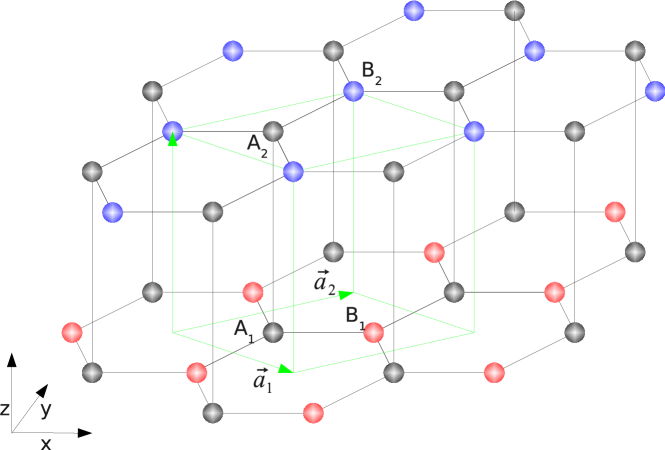
Figure 1: (Color online) Lattice structure of a graphene bilayer. The unit cell is a green parallelepiped.

The bilayer is formed by two graphene sheets, 1 and 2, arranged in the Bernal stacking. The distance between layers is 3.37 Å. Thus the unit cell of a bilayer has four atoms, its lattice structure is sketched in Fig. 1.

In addition to the intralayer parameter $\gamma_{0}$ and the interlayer parameter $t$, the corresponding Hamiltonian depends on the potential energy difference between the two layers, which we denote $2u$. The parameter $\gamma_{0}\approx 3.1$ eV yields the Fermi velocity $v_{F}\approx 1.0\times 10^{6}$ m/s, defined by $\hbar v_{F}=\gamma_{0}\sqrt{3}a/2$. We further consider that $t\approx 0.39$ eV, and the energy $2u$ varies between $0$ and $250$ meV.Zhang et al. (2009) While $\gamma_{0}$ and $t$ are fixed by nature, we assume that $u$ and $E_{F}$ are the adjustable parameters.

If we employ the continuum approximation, Wallace (1947) the Hamiltonian $H$ in the vicinity of the $K$ point can be written as

$$H=\left(\begin{array}[]{cccc}H_{B_{2}B_{2}}&H_{B_{2}A_{2}}&H_{B_{2}A_{1}}&H_{B_{2}B_{1}}\\ \\ H_{A_{2}B_{2}}&H_{A_{2}A_{2}}&H_{A_{2}A_{1}}&H_{A_{2}B_{1}}\\ \\ H_{A_{1}B_{2}}&H_{A_{1}A_{2}}&H_{A_{1}A_{1}}&H_{A_{1}B_{1}}\\ \\ H_{B_{1}B_{2}}&H_{B_{1}A_{2}}&H_{B_{1}A_{1}}&H_{B_{1}B_{1}}\\ \end{array}\right),$$ (3)

where the matrix elements of the first layer are given by

$$H_{A_{1}A_{1}} = H_{B_{1}B_{1}}=-u,$$

$$H_{A_{1}B_{1}} = H^{*}_{B_{1}A_{1}}=\hbar v_{F}(k_{x}-ik_{y}).$$

Similarly, the matrix elements corresponding to the second layer read

$$H_{A_{2}A_{2}} = H_{B_{2}B_{2}}=u,$$

$$H_{A_{2}B_{2}} = H^{*}_{B_{2}A_{2}}=\hbar v_{F}(k_{x}+ik_{y}).$$

There are only two nonzero interlayer matrix elements

$$H_{A_{1}A_{2}}=H_{A_{2}A_{1}}=t.$$

The Hamiltonian $H^{\prime}$ in the vicinity of the $K^{\prime}$ point has a similar structure, the matrix elements of $H^{\prime}$ are complex conjugates of the matrix elements of $H$.

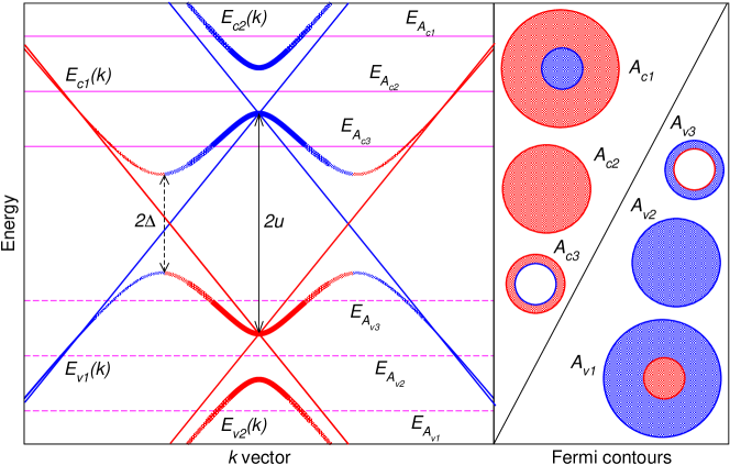
Figure 2: (Color online) The ,,mexican hat” shape of the valence and conduction bands of a biased bilayer. The blue and red colors correspond to higher probability of finding charge carriers in the layers 1 and 2, respectively. Three groups of the Fermi contour are possible depending on the value of $E_{F}$: the double circles (A1), the circles (A2), and the Fermi rings (A3).

The above Hamiltonians can be diagonalized analytically.Pereira et al. (2007); Nilsson et al. (2008); Castro et al. (2008, 2007b); Neto et al. (2009) The zero-field energy branches of the conduction band, $E_{c1}(k)$ and $E_{c2}(k)$, and the valence band, $E_{v1}(k)$ and $E_{v2}(k)$, of a bilayer result from hybridization of Fermi cones of layers 1 and 2, mediated by the interlayer matrix element $t$. Note that $E_{v1}(k)=-E_{c1}(k)$ and $E_{v2}(k)=-E_{c2}(k)$ and that the valley degeneracy is preserved, i.e., we get the same bands in valleys $K$ and $K^{\prime}$.

For $u=0$ two Fermi cones are replaced by four bonding and antibonding hyperbolic bands. The bonding valence and conduction bands, $E_{v1}(k)$ and $E_{c1}(k)$, touch at $k=0$, the separation between bands of a bonding–antibonding pair is equal to $t$ on the energy scale.

When the interlayer voltage is applied, the Fermi cones of two layers are shifted along the energy axis, and the separation of the neutrality points becomes equal to $2u$. The hybridization due to the interlayer parameter $t$ is strongest near the cone cross-points. The resulting four bands are shown in Fig. 2. It turns out that for any finite $u$ a gap is open between the topmost valence band $E_{v1}(k)$ and the bottom conduction band $E_{c1}(k)$. The conduction band acquires a ,,mexican hat” shape with energy minima at nonzero $k$ and a local maximum at $k=0$. We can write

$$E_{c1}^{\,\,\text{max}}(0) = u,$$

$$E_{c2}^{\,\,\text{min}}(0) = \sqrt{u^{2}+t^{2}},$$

$$E_{c1}^{\,\,\text{min}}(k) = \Delta=ut/\sqrt{4u^{2}+t^{2}}.$$ (4)

Note that for large $k$ the band $E_{c1}(k)$ describes electrons localized mostly in the layer 1. Near the local maximum at $k=0$ the holes in the layer 2 prevail. Similar conclusions can be drawn for the topmost valence band $E_{v1}(k)$.

As mentioned in Introduction, the quasiclassical frequencies of the bilayer, $F_{1}$ and $F_{2}$, are proportional to areas surrounded by the Fermi circles, which depend, for a given $u$, on the Fermi energy value $E_{F}$. Three different possibilities are depicted in Fig. 2 for the case of conduction/valence bands. (For the valence bands $E_{F}$ should be replaced by $-E_{F}$.)

The analytic expressions for the quasiclassical frequencies $F_{1}$ and $F_{2}$ read

$$F_{1(2)}=\frac{2\hbar}{3|e|a^{2}\gamma_{0}^{2}}\left[E_{F}^{2}+u^{2}\pm\sqrt{(E_{F}^{2}-u^{2})t^{2}+4E_{F}^{2}u^{2}}\right],$$ (5)

the frequencies $F_{1(2)}$ are even functions of variables $E_{F}$ and $u$. The frequency $F_{2}$ is equal to zero at the local maximum $E_{c1}^{\,\,\text{max}}(0)$, and at the minimum $E_{c2}^{\,\,\text{min}}(0)$. For a finite $u$, the frequency $F_{2}$ approaches $F_{1}$ at $E_{c1}^{\,\,\text{min}}(k)$.

Three forms of the Fermi contour are possible depending on the value of $E_{F}$. First, the large $E_{F}$ cuts both conduction bands and $F_{1}>F_{2}>0$. The frequency $F_{1}$ corresponds to electron orbits localized mainly in the layer 1, the frequency $F_{2}$ corresponds to hole orbits localized mainly in the layer 2. Second, only the band $E_{c1}$ is cut by $E_{F}$. Then $F_{1}>0$ and $F_{2}<0$. In this case $F_{2}$ is just a parameter and does not have the meaning of a true frequency. At last, the $E_{F}$ cuts the bottom conduction band $E_{c1}(k)$ twice, if it is less than a local energy maximum, $E_{c1}^{\,\,\text{max}}(0)$. Then again $F_{1}>F_{2}>0$. In that case $F_{1}$ is the frequency of an electron orbit in the layer 1 while $F_{2}$ belong to a hole orbit in the layer 2. Close to the local minima the difference between electrons and holes is smeared and charge carriers are present in both layers as indicated by the change of line colors in Fig. 2.

For the special case of $u=0$, Eq. (5) reduces to

$$F_{1(2)}=\frac{2\hbar}{3|e|a^{2}\gamma_{0}^{2}}\left(E_{F}\pm t\right)E_{F}.$$ (6)

Then the gap between the valence and conduction bands as well as the local maximum $E_{c1}^{\,\,\text{max}}(0)$ all disappear.

The quasiclassical phases of MOs are not accesible via the Onsager-Lifshitz quantization rule, Eqs. (1) and (2). To find the energy spectra beyond the quasiclassical approximation, we need to diagonalize the magnetic Hamiltonians $H$ and $H^{\prime}$.

III Magnetic field effects

The magnetic Hamiltonians can be obtained from the zero-field Hamiltonians by modification of matrix elements $H_{A_{1}B_{1}}$, $H_{B_{1}A_{1}}$, $H_{A_{2}B_{2}}$ and $H_{B_{2}A_{2}}$.McClure (1960); Inoue (1962); Pereira et al. (2007) The matrix elements of the magnetic Hamiltonian in the vicinity of the $K$ point are

$$H_{A_{1}B_{1}} = H^{*}_{B_{1}A_{1}}=\sqrt{2|e|\hbar v_{F}^{2}B\,n},$$

$$H_{A_{2}B_{2}} = H^{*}_{B_{2}A_{2}}=\sqrt{2|e|\hbar v_{F}^{2}B\,(n+1)}.$$

The other matrix elements remain the same as in the zero-field Hamiltonian. Near the $K^{\prime}$ point,

$$H^{\prime}_{A_{1}B_{1}} = H^{\prime*}_{B_{1}A_{1}}=\sqrt{2|e|\hbar v_{F}^{2}B\,(n+1)},$$

$$H^{\prime}_{A_{2}B_{2}} = H^{\prime*}_{B_{2}A_{2}}=\sqrt{2|e|\hbar v_{F}^{2}B\,n}.$$

We need not diagonalize these Hamiltonians to construct the Landau plot. If we look for magnetic fields $B_{n}$ at which the LLs cross $E_{F}$, it is enough to find the poles of the resolvent $G(z)=(z-H)^{-1}$, as it defines the density of states $g(E_{F})$ through

$$g(E_{F})\propto-\frac{1}{\pi}\,{\mathcal{I}m}\,{\text{T}r}\,G(E_{F}+i0).$$ (7)

The easiest way to find the poles is to solve the corresponding secular equation for $B_{n}$ assuming the fixed $E_{F}$.

We start with the simplest case of the unbiased BLG ($u=0$). Then the secular equations can be given a very convenient form, utilizing the quasiclassical frequencies of MOs, presented in the previous paragraph, Eq. (6),

$$B^{2}n(n+1)-B\left(n+\frac{1}{2}\right)(F_{1}+F_{2})+F_{1}F_{2}=0.$$ (8)

The Hamiltonians $H$ and $H^{\prime}$ yield identical equations for valleys $K$ and $K^{\prime}$.

While the secular polynomial is quartic in energy it is only quadratic in $B$. Therefore, to construct the Landau plot it is enough to solve the quadratic equation to find $B_{n}$ in terms of fixed $E=E_{F}$,.

The quasiclassical phase $\gamma$ can be easily obtained from Eq. (8). For a large number of LLs below $E_{F}$ one may assume that $n(n+1)\rightarrow(n+1/2)^{2}$, and then Eq. (8) can be written in the form

$$B^{2}\left(n+\frac{1}{2}\right)^{2}-B\left(n+\frac{1}{2}\right)(F_{1}+F_{2})+F_{1}F_{2}=0.$$ (9)

From here we obtain the asymptotic quasiclassical Landau plots

$$\frac{F_{1(2)}}{B_{n}}=n+\frac{1}{2},$$ (10)

i.e., we found that the phases of MOs correspond to SFs with $\gamma=1/2$, in agreement with quasiclassical treatments of systems with inversion symmetry. Note that $F_{2}$ is positive only in the rather unrealistic case $|E_{F}|>t$.

To get Landau plots for an arbitrary $n$ we can express the solution of Eq. (8) as

$$\frac{2F_{1}F_{2}}{F_{1}+F_{2}}\frac{1}{B_{n}}=n+\frac{1}{2}\mp\sqrt{\left(n+\frac{1}{2}\right)^{2}-n(n+1)\frac{4F_{1}F_{2}}{(F_{1}+F_{2})^{2}}}$$ (11)

or, if we define dimensionless $\delta$ by

$$\delta=\left(\frac{F_{1}-F_{2}}{F_{1}+F_{2}}\right)^{2},$$ (12)

we can write (see also Ref. Smrčka and Goncharuk, 2009)

$$\frac{F_{1(2)}}{B_{n}}=\frac{n+\frac{1}{2}\mp\sqrt{\frac{1}{4}+n(n+1)\delta}}{1\mp\sqrt{\delta}}.$$ (13)

Here the negative sign in the numerator/denominator corresponds to the frequency $F_{1}$ in the quasiclassical limit, and the positive sign to the quasiclassical frequency $F_{2}$. It is obvious that for $\delta\neq 0$ the MOs are not periodic in $1/B$.

The case of the biased BLG ($u\neq 0$) must be treated separately, as the presence of the electric field perpendicular to layer planes breaks the inversion symmetry and lifts the valley degeneracy.Mucha-Kruczyński et al. (2009); Nakamura et al. (2009)

The secular equations can be given again a form quadratic in $B$, but the coefficients do not depend exclusively on the quasiclassical frequencies as in Eq. (8). We can write

$$B^{2}n(n+1)-B\left[(n+\frac{1}{2})(F_{1}+F_{2})+F_{0}\right]+F_{1}F_{2}=0$$ (14)

for the Hamiltonian $H$ in the vicinity of $K$. In comparison with Eq. (8) there is an extra term

$$F_{0}=\frac{4\hbar}{3|e|a^{2}\gamma_{0}^{2}}E_{F}u.$$ (15)

In the vicinity of $K^{\prime}$ we obtain a very similar equation from the Hamiltonian $H^{\prime}$, the only difference is that $F_{0}$ is replaced by $-F_{0}$. The extra term, $F_{0}$, is the reason of the valley asymmetry. It is obvious that Eq. (14) gives two different series of solutions, $B_{n}$, for positive and negative $F_{0}$.

The quasiclassical frequencies $F_{1}$ and $F_{2}$ are even functions of $E_{F}$ and $u$. It means that there are the same frequencies not only for $K$ and $K^{\prime}$, but also for the electrons and holes with energies $E_{F}$ and $-E_{F}$, respectively. Note also that $F_{1}$ and $F_{2}$ do not depend on the sign of $u$. On the other hand, $F_{0}$ is an odd function of $E_{F}$ and $u$. Thus $F_{0}$ breaks the $K$ – $K^{\prime}$ symmetry, and also the symmetry between the electron and hole oscillations with the same quasiclassical frequencies. The change of sign of $u$ also reverts the roles of $K$ and $K^{\prime}$ valleys, i.e., what is valid for $K$ with $u>0$ is valid for $K^{\prime}$ with $u<0$.

Also Eq. (14) can be rewritten to an equation similar to Eq. (13), but with an additional dimensionless parameter $\lambda$, which depends on $F_{0}$,

$$\lambda=\frac{F_{0}}{F_{1}+F_{2}}.$$ (16)

Then the analytic solution reads

$$\frac{F_{1(2)}}{B_{n}}=\frac{n+\frac{1}{2}+\lambda\mp\sqrt{(n+\frac{1}{2}+\lambda)^{2}+n(n+1)(1-\delta)}}{1\pm\sqrt{\delta}}.$$ (17)

This equation reduces to Eq. (13) for $\lambda=0$.

Now it is a more difficult task to find an asymptotic expression for the oscillation phase than in the previous case $u=0$. If we solve Eq. (14) for $n+1/2$ we get

$$n+\frac{1}{2}=\frac{F_{1}+F_{2}\pm\sqrt{(F_{1}-F_{2})^{2}+4BF_{0}+B^{2}}}{2B},$$ (18)

which for $B$ approaching zero yields

$$\frac{F_{1(2)}}{B}=n+\frac{1}{2}\mp\xi.$$ (19)

Here $\xi$ is a gate-tunable correction to the oscillation phase, given by

$$\xi=\frac{F_{0}}{F_{1}-F_{2}}=\frac{E_{F}u}{\sqrt{(E_{F}^{2}-u^{2})t^{2}+4E_{F}^{2}u^{2}}}.$$ (20)

This correction differs in sign for $K$ and $K^{\prime}$ and also differs for electrons and holes from the same valley with the same absolute value of energy.

IV Results and discussion

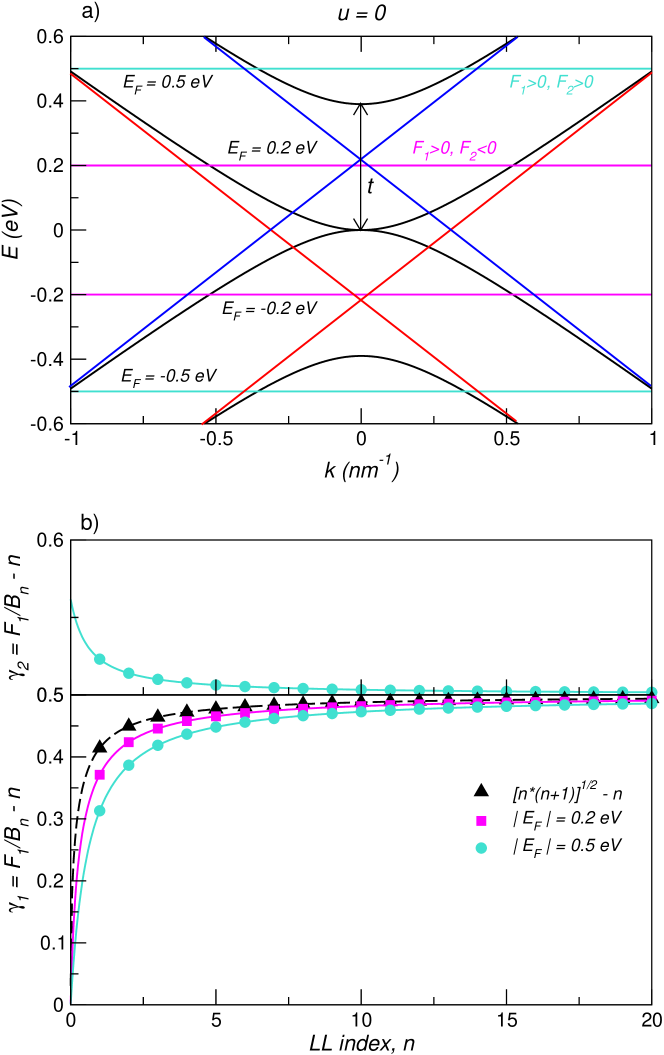
Figure 3: (Color online) (a) The electronic bands of the unbiased graphene bilayer ($u=0$). The horizontal lines denote the Fermi energies which cross the electron and hole dispersion curves. (b) The ,,phases” $\gamma_{1(2)}(E_{F})=F_{1(2)}/B-n$, for $E_{F}$ depicted in a), plotted as functions of the Landau level index $n$.

In the unbiased BLG the energy $u$ is equal to zero and the parameter $\delta$, which appears in Eq. (13), has a particularly simple form

$$\delta=\frac{t^{2}}{E_{F}^{2}}.$$ (21)

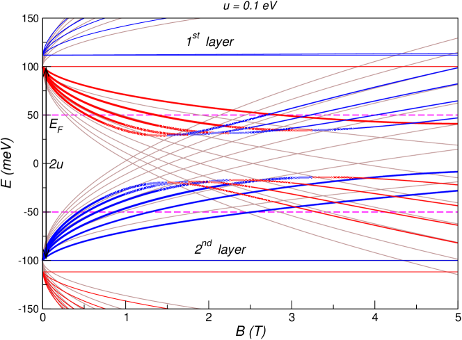
Figure 4: (Color online) The electron and hole Landau levels (in the $K^{\prime}$ valley) of two layers are mixed by the interlayer interaction, $t$. For the energy range corresponding to Fermi rings in zero magnetic filed (see $A_{3}$ in Fig. 2), $E_{F}$ cuts the Landau levels twice. This is the reason for the anomalous phase in the quasiclassical limit $B\rightarrow 0$.

For small Fermi energies only the bottom branch $E_{c1}(k)$ of the conduction subband is cut by $E_{F}$ and only the frequency $F_{1}$ is defined. For $E_{F}$ approaching zero, the parameter $\delta$ diverges. This implies that for energies close to the band bottom Eq. (13) can be written as

$$\frac{F_{1}}{B}=\sqrt{n(n+1)},$$ (22)

the form found for the extremal electron and hole orbits in graphite,Smrčka and Goncharuk (2009) which clearly indicates the aperiodicity of oscillations.

The Fermi energies greater than $t$ are rather unrealistic. Nevertheless we can consider this hypothetical case in our theoretical treatment. We can write, for $E_{F}=t$ and $\delta=1$, Eq. (13) as follows

$$\frac{F_{1}}{B} = \frac{n(n+1)}{n+\frac{1}{2}},$$ (23)

$$\frac{F_{1}}{B} = n+\frac{1}{2}.$$

The Landau plots calculated for two selected values of $E_{F}$, $E_{F}<t$ and $E_{F}>t$, which cross the dispersion curves are presented in Fig. 3. The Landau plots are the same for $E_{F}$ and $-E_{F}$ due to the inversion symmetry conservation. One can observe that in the unbiased bilayer the phases of MOs, corresponding to both frequencies $F_{1}$ and $F_{2}$, approach the phase of massive fermions,$\gamma=1/2$, for higher quantum numbers of LLs.

In BLG, an applied electric field leads to asymmetry between $K$ and $K^{\prime}$ valleys that gives rise to nontrivial oscillation phenomena in magnetic fields. To illuminate an anomalous behavior of oscillations, we plotted in Fig. 4 the field dependence of LLs in BLG.

In a single layer graphene the LL fans of electrons and holes start at the zero-field neutrality point. The neutrality points of two independent layers are shifted by $2u$ and the LLs of holes from the layer 1 cross the LLs of electrons from the layer 2, as shown in Fig. 4 by thin brown lines.

In BLG the shape of LL spectrum results from hybridization of LL spectra of layers 1 and 2. Due to the interlayer interaction, represented by the matrix element $t$, we have four fans of LLs which start at zero-field energies $E_{v2}(0)$, $E_{v1}(0)$, $E_{c1}(0)$ and $E_{c2}(0)$.

The hole levels from the layer 1 and the electron levels from the layer 2 avoid to cross, and the low-field hole LLs smoothly turn into the electron LLs as $B$ increases. This is indicated in Fig. 4 by the change of LL color from red to blue. The LLs from a fan starting at zero-field energy $E_{c1}(0)$ have minima in their field dependence and, therefore, can be cut twice by a single $E_{F}$. Moreover, the minima are not the same for all levels and, consequently, not all levels are cut by a single $E_{F}$.

This is reflected in the quasiclassical approach as the gate-dependent correction to the MO phase, $\xi$, which is related to the energy difference $2u$ between two layers. Note that in the region of energies corresponding to the Fermi rings the expression (20) diverges at $E_{c1}^{\,\,\text{min}}(k)$ and is equal to $1/2$ for $E_{F}=E_{c1}^{\,\,\text{max}}(0)$. As the many body effects can play a role in this low concentration range, the above one-electron picture is probably oversimplified.

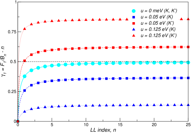
Figure 5: (Color online) The ,,phase” $\gamma_{1}=F_{1}/B-n$ calculated for the fixed quasiclassical frequency $F_{1}=70$ T and various $u$, for the electron $K$ and $K^{\prime}$ valleys as a function of the LL index, $n$.

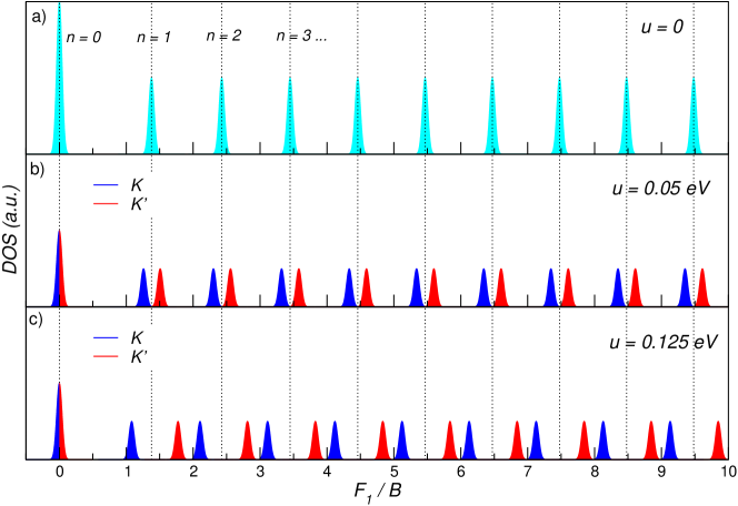
Figure 6: (Color online) The DOS of the unbiased (a) and biased (b, c) BLG versus dimensionless value of the Landau plot, $F_{1}/B$, with the fixed quasiclassical frequency $F_{1}=70$ T. The frequency $F_{1}$ corresponds to the situation when $F_{1}>0,F_{2}<0$, i.e., only the lowest conduction/valence energy band is cut by $E_{F}$. In (b, c) the blue peaks show DOS calculated for the $K$ valley, whereas the red ones are related to the $K^{\prime}$ valley.

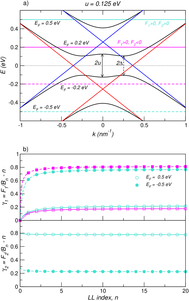
Figure 7: (Color online) (a) The electron/hole bands of the biased graphene bilayer with the gap $2u=0.25$ eV at $k=0$. The horizontal lines denote the Fermi energies which cross the electron (solid lines) and hole (dashed lines) dispersion curves. (b) The ,,phases” $\gamma_{1(2)}(E_{F})=F_{1(2)}/B-n$ calculated for $E_{F}$ depicted in (a) plotted as functions of the LL index, $n$.

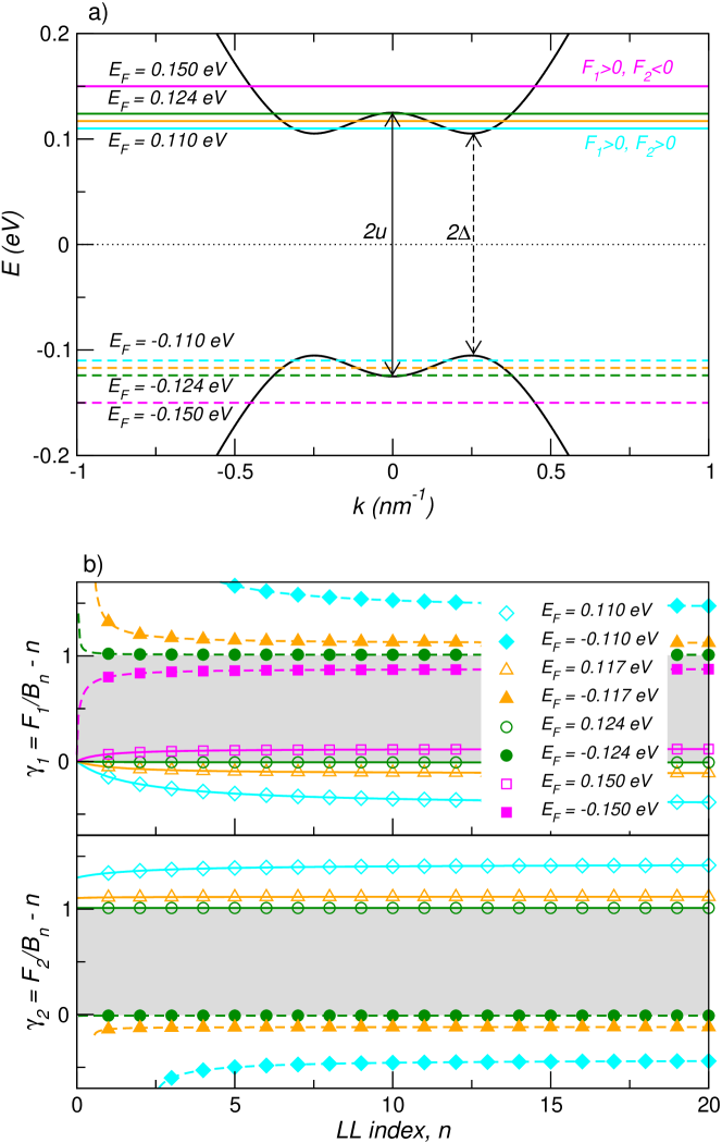
Figure 8: (Color online) The same as in Fig. 7, only for the lowest electron/hole bands and $\Delta<|E_{F}|<u$.

We start our discussion with the simplest case, $E_{c1/v1}(0)<|E_{F}|<E_{c2/v2}(0)$, when only one conduction/valence energy band is cut by $E_{F}$ (see Fig. 2). The single quasiclassical frequency $F_{1}$ corresponds to a single Fermi area, which is the same for $K$ and $K^{\prime}$.

According to Eq. (19), the electron peaks in DOS are shifted by $\xi$ to the left in the $K$ valley, whereas the peaks in the $K^{\prime}$ valley are shifted by $\xi$ to the right. The shift magnitude ranges from zero to $1/2$ depending on the energy difference between two layers. In Fig.5 the ,,phase” $\gamma_{1}$ is plotted as the function of $n$ for three different cases with $u$ equal to 0, 0.05 and 0.125 eV. The Fermi energies are chosen to keep the same Fermi area (and the same fixed $F_{1}$) in all three systems. Only for $u=0$ the curves are identical for $K$ and $K^{\prime}$, for $u\neq 0$ the curves are substantially different.

In Fig. 6 the shifts of peaks in the above three cases are shown explicitly. There is a single series of oscillations for the unbiased bilayer, as the valley degeneracy is preserved in a system with the inversion symmetry.

The effect of the gate-tunable valley splitting originates in two series of oscillations which differ for the different $u$. Let us emphasize that all series of oscillations have the same quasiclassical frequency $F_{1}$, but the quasiclassical phases depend on the choice of $u$ and on the choice of the valley index.

We complete our discussion with cases when the Fermi energy cuts the conduction/valence bands twice. The Landau plots of the biased bilayer with $u=0.125$ eV, which is probably the highest experimentally accessible value, Zhang et al. (2009) calculated for four selected Fermi energies, two in the conduction band, and two in the valence band, are presented in Fig. 7. In accordance with types of the Fermi contours in Fig. 2, the first and second cases are depicted.

The situation is more complicated in the region of energies, $\Delta<|E_{F}|<u$, for which $E_{F}$ cuts the lowest subband $E_{c1/v1}(k)$ twice, which is characteristic for the third type of the Fermi contours, as shown in Fig. 2. The bottom of $E_{c1}(k)$ is at $\approx 0.105$ eV. The parameter $\xi$ is far from the values expected for the phase of quasiclassical oscillations, it reduces/grows heavily when $E_{F}$ approaches the bottom of $E_{c1}(k)$/$E_{v1}(k)$. For $E_{F}=u$, $\xi$ becomes closer to $-1/2$ for $E_{F}$ in the conduction band and $1/2$ for $E_{F}$ in the valence band.

V Conclusions

Using a four-band continuum model, we calculated analytically the Landau plots in biased and unbiased BLG subject to external perpendicular magnetic fields.

It turns out that the magneto-oscillations are only asymptotically periodic, and that in the unbiased bilayers their phase is equal to the phase of massive fermions. The convergence to the quasiclassical limit is slow, and depends strongly on the the value of $E_{F}$. The convergence is slower for higher values of $E_{F}$.

Anomalous behavior of oscillation phases was found in biased bilayers with broken inversion symmetry. The oscillation frequencies again tend to quasiclassically predicted ones, which are the same for $K$ and $K^{\prime}$, but the quantum approach yields the gate-tunable corrections to oscillation phases, which differ in sign for $K$ and $K^{\prime}$. These valley-dependent phase corrections give rise, instead of a single quasiclassical series of oscillations, to two series with the same frequency but shifted in phase.

We also found that for $E_{F}$ in the region of energies corresponding to the Fermi rings in the quasiclassical approach, only a limited number of LLs can cut the Fermi energy and thus a limited number of magneto-oscillations can be achieved. Moreover, their quasiclassical phases reach very large values. As the many body effects can play a role in the corresponding concentration range, the above one-electron picture is probably oversimplified.