Electronic Coherence Dephasing in Excitonic Molecular Complexes: Role of Markov and Secular Approximations

Abstract

We compare four different types of equations of motion for reduced density matrix of a system of molecular excitons interacting with thermodynamic bath. All four equations are of second order in the linear system-bath interaction Hamiltonian, with different approximations applied in their derivation. In particular we compare time-nonlocal equations obtained from so-called Nakajima-Zwanzig identity and the time-local equations resulting from the partial ordering prescription of the cummulant expansion. In each of these equations we alternatively apply secular approximation to decouple population and coherence dynamics from each other. We focus on the dynamics of intraband electronic coherences of the excitonic system which can be traced by coherent two-dimensional spectroscopy. We discuss the applicability of the four relaxation theories to simulations of population and coherence dynamics, and identify features of the two-dimensional coherent spectrum that allow us to distinguish time-nonlocal effects.

I Introduction

Modeling molecular properties related to their non-equilibrium dynamics requires various theoretical approaches depending on the particular microscopic processes related to the observed molecular features. Since the dawn of quantum mechanics, properties of molecules and solids have been studied theoretically in ever greater detail. This has led in recent years to a state in which dynamics of complex systems with multitude of degrees of freedom (DOF) is accessible to quantitative theoretical study ComplexMolSystem . Many properties of molecular systems are directly related to the equilibrium or time dependent conformations of nuclear DOF for which electronic states play the role of a background contributing to the nuclear potential energy surfaces. Problems like these are the realm of molecular dynamics (MD) in its classical, quantum or mixed versions and quantum chemistry (QC), where impressive qualitative and quantitative results have been achieved in recent years. For certain types of dynamical problems, however, less expensive model approaches are the preferred choice due to the scale of studied system or due to the physical nature of studied processes. A good example of such a problem is ultrafast photo-induced excited state dynamics of small molecular systems and their aggregates PhotosynthExcitonsBook . Here, most of the relevant experimental information is only available through ultrafast non-linear spectroscopy, and thus the theory has to span the whole distance between the microscopic dynamics of the molecular system, and the macroscopic description of experimental signals MukamelBook . Typical field in which such an approach has yielded deep understanding of the relevant physico-chemical processes is the study of primary processes in photosynthesis. The related quantum mechanical problem is usually formulated in terms of a model describing the relevant DOF of the system (electronic states of photosynthetic molecules), and a thermodynamics bath (the protein environment). Parameters for such models can be supplied by experiment Renger01 , QC studies Scholes01 ; Madjet01 , MD modeling Schulten01 , or are a result of suitable simplified models MukamelBook .

Recent advances in non-linear spectroscopy have opened a wide new experimental window into the details of ultrafast photo-induced dynamics of molecular systems. Experimental realization of two-dimensional (2D) coherent spectroscopy in the visible and near IR regions Jonas01 ; Miller01 ; BrixnerStiopkin ; BrixnerMancal has enabled to overcome some of the frequency- vs. time-resolution competition problem otherwise faced by ultrafast spectroscopy, and yielded thus unprecedented experimental details of the time evolution of molecular excitations. Most importantly, it was predicted that the presence of certain oscillatory features in 2D spectra is a manifestation of coherences between molecular excited states PisliakovMancal ; Bruggemann01 . It was also concluded that these oscillations should be present in the 2D spectrum of photosynthetic Fenna-Matthews-Olson (FMO) chromophore-protein complex PisliakovMancal . Experimental results not only confirmed this prediction EngelNature , but yielded also surprising results such as unexpectedly long life time of these coherences, as compared to the predictions of standard dephasing rate theory. Furthermore, while possible coherence transfer was ignored by the relaxation theory used in Ref. PisliakovMancal , the experiment provided some evidence for its role in excitation energy transfer. It was speculated that photosynthetic systems might use the coherent mode of energy transfer to more efficiently channel excitation energy by scanning their energetic landscape in a process similar to quantum computing EngelNature . More experiments have recently reported coherent dynamics in photosynthetic systems Lee_Science and conjugated polymers Scholes02 , and the field of energy transfer in photosynthesis has seen an increased interest from theoretical researchers from previously unrelated fields Rebentrost ; Mohseni ; Plenio ; Olaya-Castro .

Theoretical basis for the description of the decoherence phenomena in excitation energy transfer has been developed long ago in the framework of the reduced density matrix (RDM) Nakajima ; Zwanzig . Equations of motion resulting from this scheme are characterized by the presence of time retarded terms responsible for energy relaxation and decoherence processes. Equations of this type will be denoted as time non-local in this paper. Later, an alternative approach to the derivation of the RDM equations of motion has emerged which yields time local equation of motion Hashitsume ; Shibata . Both theories express the relaxation term in form of an infinite series in terms of the system-bath interaction Hamiltonian, but differ in time ordering prescriptions for the cumulant expansion of the evolution operator. The time local equations correspond to so-called partial time ordering prescription of the cummulant expansion, while the time non-local equations result from so-called chronological time ordering Mukamel1 ; Mukamel2 . Although the two schemes yield formally different equations of motion for the RDM, they are in fact equivalent as long as the complete summation of the corresponding infinite series is performed. When the infinite series are truncated at a finite order, the two theories yield equations that predict different RDM dynamics. This is a result of different statistical assumptions about the bath that are implicitly made in the two cases Mukamel1 ; Mukamel2 . In all orders of expansion, so-called Markov approximation can be used to transform the time non-local equation of motion into a certain time-local form. This has to be regarded as an additional approximation which simplifies the numerical treatment of the time non-local equations. Interestingly, in the second order the time-local equations and the time non-local equations with Markov approximation have exactly the same form.

Until recently, most experiments were not sensitive to coherence between electronic levels. This allowed a host of further approximations to simplify equations of motion. Most notably, the secular approximation, which amounts to decoupling RDM elements oscillating on different frequencies from each other, has limited the energy transfer phenomena to separate dynamics of population transfer and coherence dephasing MayBook . Even on very short times scale, experiments aimed at studying population dynamics (pump probe) are not sensitive enough to coherences between electronic levels to require non-secular theory, although it was suggested that measured relaxation time can be distorted by non-secular effects Capek . Consequently, most of the theory developed for evaluation of experiments has been aimed at improving calculation of the relaxation rates Zhang ; Mino ; Silbey04 . With experiments now uncovering new details about the role of electronic coherence, theoretical methods beyond rate equations for probabilities which are both accurate and numerically tractable are required. Although schemes for constructing equations of motion for the RDM beyond second order, based on co-propagation of the RDM with auxiliary operators, seem feasible and promising Ishizaki1 ; Ishizaki2 , second order theories might still be the only option for treatment of extended molecular systems. It was suggested previously that second order perturbation theory with respect to system-bath coupling provides a suitable framework for development of such methods Mancal08a . This notion is also supported by the fact that in the special case of so-called spin-boson model, second order time-local equation of motion already represents an exact equation of motion for the RDM Haenggi08 .

In this paper we study the following four different second order theories: (a) full time non-local (full TNL) equation of motion resulting from the Nakajima-Zwanzig identity or equivalently from the chronological ordering prescription in the cummulant expansion, (b) the full time local (full TL) equation of motion resulting from the partial ordering prescription in the cummulant expansion, or equivalently from Markov approximation applied to TNL equation, (c) time non-local equation with secular approximation (secular TNL), and (d) time local equation with secular approximation (secular TL). We discuss the applicability of these equations to the description of the energy relaxation and decoherence dynamics in small systems of molecular excitons with the emphasis of on recent 2D spectroscopic experiments and the dynamics of coherence between electronic excited states. Note that, in this paper, full refers to the equations where no secular approximation has been applied. These equations are still of second order of perturbation theory.

The paper is organized as follows. The next section introduces Hamiltonian description of an aggregate of small molecules embedded in a protein or solid state environment. In Section III we describe the details of second order theory of system–bath interaction and we derive four different equations of motion for the RDM describing electronic states of a molecular aggregate. Two-dimensional coherent spectroscopy, and non-linear spectroscopy in general are introduced in Section IV. In Section V we present and discuss numerical results comparing different theories of relaxation on calculations of coherence life time and 2D spectra.

II Model Hamiltonian

The investigated molecular system is an aggregate composed of $N$ monomers embedded in protein environment. Let us first consider a monomeric molecule (a chromophore) embedded in the environment, but insulated from interaction with its neighboring monomers. The monomer Hamiltonian has a form

$$H^{m}=\left(\varepsilon_{g}^{(m)}+T(P_{m})+V_{g}^{(m)}(Q_{m})\right)|g_{m}\rangle\langle g_{m}|$$

$$+\left(\varepsilon_{e}^{(m)}+T(P_{m})+V_{e}^{(m)}(Q_{m})\right)|e_{m}\rangle\langle e_{m}|\;,$$ (1)

where $|g_{m}\rangle$, $|e_{m}\rangle$ denote electronic ground and excited states, and $\varepsilon_{g}^{(m)}$, $\varepsilon_{e}^{(m)}$ represent electronic energies of these states. The kinetic term $T(P_{m})$ and the potential terms $V_{g}^{(m)}(Q_{m})$, $V_{e}^{(m)}(Q_{m})$ represent the intra-molecular DOF and the protein environment (bath or reservoir) interacting with these states. By $Q_{m}$ $(P_{m})$ we denote the (possibly macroscopic) set of coordinates (impulses) describing both the intramolecular nuclear DOF of the $m$-th monomer as well as the DOF of its surroundings. The total Hamiltonian of the monomer can be split into the system, reservoir and the system-reservoir coupling terms

$$H_{S}^{m}\equiv\varepsilon_{g}^{(m)}|g_{m}\rangle\langle g_{m}|$$

$$+(\varepsilon_{e}^{(m)}+\langle V_{e}^{(m)}(Q_{m})-V_{g}^{(m)}(Q_{m})\rangle_{eq})|e_{m}\rangle\langle e_{m}|\;,$$ (2)

$$H_{\mathrm{R}}^{m}\equiv[T(P_{m})+V_{g}^{(m)}(Q_{m})]$$

$$\times\left(|g_{m}\rangle\langle g_{m}|+|e_{m}\rangle\langle e_{m}|\right)$$

$$=[T(P_{m})+V_{g}^{(m)}(Q_{m})]\otimes\hat{1},$$ (3)

$$H_{\mathrm{S-R}}^{m}\equiv\Big{(}V_{e}^{(m)}(Q_{m})-V_{g}^{(m)}(Q_{m})$$

$$-\langle V_{e}^{(m)}(Q_{m})-V_{g}^{(m)}(Q_{m})\rangle_{eq}\Big{)}|e_{m}\rangle\langle e_{m}|$$

$$\equiv\Delta\Phi_{m}(Q_{m})|e_{m}\rangle\langle e_{m}|\;.$$ (4)

Here, $\langle A(Q)\rangle_{eq}$ represents averaging of an arbitrary $Q-$dependent operator over equilibrium state of the bath. By this choice of the splitting we have assured that $\Delta\Phi^{(m)}(Q_{m})=0$ for the system in equilibrium. To simplify the notation, we redefine electronic energy of the excited state to include the equilibrium average of the potential energy difference between the electronic excited and ground states, $\tilde{\varepsilon}_{e}^{(m)}=\varepsilon_{e}^{(m)}+\langle V_{e}^{(m)}(Q_{m})-V_{g}^{(m)}(Q_{m})\rangle_{eq}$ and we drop the tilde over $\varepsilon_{e}^{(m)}$ further in this paper.

An aggregate built out of these monomers can be represented on a Hilbert space composed of collective aggregate states. We define the aggregate ground state

$$|g\rangle=\prod_{m=1}^{N}\otimes|g_{m}\rangle,$$ (5)

states with a single excitation

$$|u_{n}\rangle=\prod_{m=1}^{n-1}\otimes|g_{m}\rangle\otimes|e_{n}\rangle\prod_{m^{\prime}=n+1}^{N}\otimes|g_{m^{\prime}}\rangle,$$ (6)

and multi-excited states in an analogical manner. We drop the sign $\otimes$ in further consideration for the sake of brevity. The Hamiltonian of the aggregate is constructed using the energies of collective states

$$H_{S}^{non-int}=\varepsilon_{g}|g\rangle\langle g|$$

$$+\sum_{n}\left(\Delta\varepsilon_{n}+\Omega\right)|u_{n}\rangle\langle u_{n}|+\mathrm{h.\;e.\;t.},$$ (7)

where $\varepsilon_{g}=\sum_{n}\varepsilon_{g}^{(n)}$, $\Omega=N^{-1}\sum_{n}\varepsilon_{e}^{(n)}$, and $\Delta\varepsilon_{n}=\varepsilon_{e}^{(n)}-\Omega+\sum_{m\neq n}\varepsilon_{g}^{(m)}$. The abreviation h. e. t. denotes higher excitonic terms. Due to the fact that the monomers are positioned in a tight aggregate, we have to account for the interaction energy between their excited states. The interaction energy between states $|u_{m}\rangle$ and $|u_{n}\rangle$ will be denoted $J_{mn}$, and the corresponding contribution to the total Hamiltonian reads

$$H_{S}^{int}=\sum_{n\neq m}\left(J_{nm}|u_{n}\rangle\langle u_{m}|+\mathrm{c.c}.\right)+\mathrm{h.\;e.\;t.}.$$ (8)

Due to the off-diagonal terms $J_{mn}$ the collective states defined in Eq. (6) are not eigenstates of the total Hamiltonian $H_{S}=H_{S}^{non-int}+H_{S}^{int}$. Although the basis of the states $|g\rangle$, $|u_{n}\rangle$ and multiple-excitation states of the aggregate provides efficient means for defining the Hamiltonian, it is more practical to switch into the basis of eigenstates of the Hamiltonian $H_{S}$. One of the reasons is that while matter interacts with light, the differences between eigenenergies of $H_{S}$ define the resonant transition frequencies. The system–bath coupling part of the aggregate Hamiltonian reads

$$H_{S-B}=\sum_{n}\Delta\Phi_{n}|u_{n}\rangle\langle u_{n}|+\mathrm{h.\;e.\;t.},$$ (9)

and thus no terms in the total Hamiltonian couple the ground state with the first excited state or higher excited state bands. In fact, the total Hamiltonian splits into blocks separated approximately by the energy $\hbar\Omega$ (see Fig. 1). This reflects the neglecting of all adiabatic couplings, which are supposed to be so weak that they do not lead to transitions on the time scale of interest (femto and picoseconds). This property is well justified e.g. for chlorophyll systems.

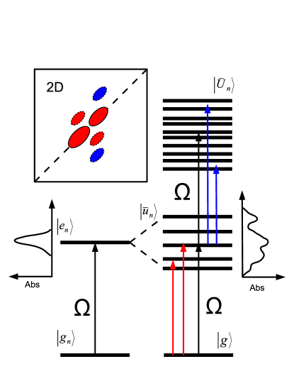
Figure 1: Illustration of the level structure of an excitonic system. The excited states $|e_{n}\rangle$ of $N$ monomers with transition frequency $\Omega$ (left part of the figure) split due to the resonance interaction into $N$ one exciton states $|\bar{u}_{n}\rangle$ (right). Absorption spectra of ensembles of non-interacting (left) and interaction (right) monomers. The system also exhibits higher excitons states (two-exciton states $|\bar{U}_{n}\rangle$ are depicted here), with $\Omega$ being the mean transition frequency from the one- to two-exciton bands. A pictorial 2D spectrum with peaks resulting from transitions between the ground- and one-exciton states (red arrows) and one- and two-exciton states (blue arrows) is presented in the upper left corner of the figure. The transitions between the ground- and one-excitons states lead to positive contributions to the 2D spectrum (absorption and ground state bleach), while the transitions between the one- and two-exciton states result in a negative contribution (excited state absorption).

For the subsequent use in this paper, we denote the eigenstates of the total electronic Hamiltonian $H_{S}$ by $|\bar{u}_{a}\rangle$, $a=1,\dots,N$, for single exciton states formed as linear combinations of single excitation states $|u_{n}\rangle$ and $|\bar{U}_{a}\rangle$, $a=N+1,\dots,N+N(N-1)/2$, for two-exciton states formed from the linear combination of pairs of single excitation states.

III Second order relaxation theories

In this section we consider interaction of the electronic system described by the Hamiltonian $H_{S}$ with a macroscopic bath composed of the DOF of the molecular surroundings.

III.1 Projection operator technique and Nakajima-Zwanzig identity

We start with the density operator $W$, which describes the state of the system composed of the aggregate and its surroundings. This operator fulfills Liouville-von Neumann equation

$$\frac{\partial}{\partial t}W(t)=-\frac{i}{\hbar}[H,W(t)]_{-}=-i{\cal L}W(t).$$ (10)

Here, $[A,B]_{-}\equiv AB-BA$, and we introduced Liouville superoperator ${\cal L}$ by its action on an arbitrary operator $A$ as ${\cal L}A=\frac{1}{\hbar}[H,A]_{-}$. Liouville superoperators ${\cal L}_{S}$, ${\cal L}_{B}$ and ${\cal L}_{S-B}$ that correspond to Hamiltonian operators of the system, the bath and their interaction will be used later in this paper. A formal solution of Eq. (10) can be written using evolution superoperators such that

$$W(t)={\cal U}(t-t_{0})W(t_{0}).$$ (11)

We are often not interested in the complete information carried by $W(t)$, but only in the information related to the electronic states of the aggregate. The reduced density matrix (RDM) defined as

$$\rho(t)=tr_{B}\{W(t)\},$$ (12)

where $tr_{B}$ represents trace over all bath DOF, is the quantity carrying just the relevant information MayBook . To derive equation of motion for $\rho(t)$ we can use projection operator approach as following. We define a projection operator ${\cal P}$ by its action on an arbitrary operator $A$ as

$${\cal P}A=tr_{B}\{A\}w,$$ (13)

where $w$ is a pure bath operator satisfying the condition $tr_{B}\{w\}=1$. For convenience we also define a complementary projection operator ${\cal Q}\equiv 1-{\cal P}$. For the projected density matrix ${\cal P}W(t)$ one can write a formally exact equation of motion as

$$\frac{\partial}{\partial t}{\cal P}W(t)=-i{\cal P}{\cal L}_{I}(t){\cal P}W(t)$$

$$-{\cal P}{\cal L}_{I}(t)\exp\left\{-i\int_{t_{0}}^{t}d\tau{\cal Q}{\cal L}_{I}(\tau){\cal Q}\right\}{\cal Q}W(t_{0})$$

$$-\int\limits_{0}^{t-t_{0}}d\tau^{\prime}{\cal P}{\cal L}_{I}(t)\exp\left\{-i\int_{t_{0}}^{\tau^{\prime}}d\tau^{\prime\prime}{\cal Q}{\cal L}_{I}(\tau^{\prime\prime}){\cal Q}\right\}$$

$$\times{\cal Q}{\cal L}_{I}(t-\tau^{\prime}){\cal P}W(t-\tau^{\prime}),$$ (14)

where the subscript _I denotes interaction picture with respect to the bath Hamiltonian $H_{B}$. Eq. (14) is known as Nakajima-Zwanzig identity MayBook ; FainBook . Although one cannot practically solve Eq. (14), because it is as difficult as the original complete problem, one can use it as a starting point for approximations that will follow.

III.2 Convolutionless equation of motion

Before we introduce approximations into Eq. (14), we can make one more formal step, which enables us to overcome its time non-local character. Let us assume an evolution superoperator ${\cal U}^{\prime}(t)$, which satisfies

$${\cal P}W(t)={\cal U}^{\prime}(t-t_{0}){\cal P}W(t_{0}).$$ (15)

This superoperator is of course unknown, but it allows us to turn a time non-local differential equation (14) formally into a time-local one. We can write

$$\frac{\partial}{\partial t}{\cal P}W(t)=-i{\cal P}{\cal L}_{I}(t){\cal P}W(t)$$

$$-{\cal P}{\cal L}_{I}(t)\exp\left\{-i\int_{t_{0}}^{t}d\tau{\cal Q}{\cal L}_{I}(\tau){\cal Q}\right\}{\cal Q}W(t_{0})$$

$$-\Big{[}\int\limits_{0}^{t-t_{0}}d\tau^{\prime}{\cal P}{\cal L}_{I}(t)\exp\left\{-i\int_{t_{0}}^{\tau^{\prime}}d\tau^{\prime\prime}{\cal Q}{\cal L}_{I}(\tau^{\prime\prime}){\cal Q}\right\}$$

$$\times{\cal Q}{\cal L}_{I}(t-\tau^{\prime}){\cal U}^{\prime}(-\tau^{\prime})\Big{]}{\cal P}W(t).$$ (16)

We do not develop the convolutionless (or time local) theory any further in this paper, because we will be interested only in terms up to the second order in ${\cal L}_{I}$. In such a case ${\cal U}^{\prime}(-\tau)$ can be approximated as ${\cal U}^{\prime}(-\tau)\approx{\cal U}_{S}(-\tau){\cal U}_{B}(-\tau)$, where ${\cal U}_{S}(-\tau)$ and ${\cal U}_{B}(-\tau)$ are evolution superoperators with respect to ${\cal L}_{S}$ and ${\cal L}_{B}$. Interested reader can refer e.g. to Refs. FainBook ; Mukamel1 ; Mukamel2 for further details.

III.3 System-Bath Coupling

We will now assume the interaction Hamiltonian in a form of Eq. (9) where index $n$ now runs through all relevant single-exciton and multi-exciton states

$$H_{I}=\sum_{n}\Delta\Phi_{n}K_{n}.$$ (17)

Correspondingly, $K_{n}=|u_{n}\rangle\langle u_{n}|$ for single excitonic states. Expanding Eqs. (14) and (16) into the second order in $H_{I}$ we find that the third term on the right hand side (r. h. s.) can be conveniently expressed via so-called bath (or energy gap) correlation functions defined as

$$C_{mn}(\tau)=tr_{Q}\{U_{B}(-\tau)\Delta\Phi_{m}U_{B}(\tau)\Delta\Phi_{n}w_{eq}\}.$$ (18)

Here, we have chosen a specific form of the bath density matrix $w\equiv w_{eq}$, where $w_{eq}$ is the canonical density matrix of the bath DOF. Defining also an operator

$$\Lambda_{m}(\tau)=\sum_{n}C_{mn}(\tau)U_{S}(\tau)K_{n}U_{S}^{\dagger}(\tau)$$ (19)

and a superoperator ${\cal M}^{(2)}(\tau)$ such that

$${\cal M}^{(2)}(\tau)A=\sum_{m}[K_{m},\Lambda_{m}(\tau)U_{S}(\tau)AU_{S}(-\tau)$$

$$-U_{S}(\tau)AU_{S}(-\tau)\Lambda_{m}^{\dagger}(\tau)]_{-},$$ (20)

the Eqs. (14) and (16) can be rewritten as

$$\frac{\partial}{\partial t}\rho(t)=-i{\cal L}_{S}\rho(t)$$

$$-\sum_{m}\int\limits_{0}^{t-t_{0}}d\tau[K_{m},\Lambda_{m}(\tau)\rho(t)-\rho(t)\Lambda_{m}^{\dagger}(\tau)]_{-}$$ (21)

and

$$\frac{\partial}{\partial t}\rho(t)=-i{\cal L}_{S}\rho(t)$$

$$-\sum_{m}\int\limits_{0}^{t-t_{0}}d\tau[K_{m},\Lambda_{m}(\tau)U_{S}(\tau)\rho(t-\tau)U_{S}(-\tau)$$

$$-U_{S}(\tau)\rho(t-\tau)U_{S}(-\tau)\Lambda_{m}^{\dagger}(\tau)]_{-}.$$ (22)

Provided we can supply a model for the correlation function $C_{mn}(\tau)$ we are in position to write down the equations of motion for RDM in terms of known quantities. The last step necessary to implement these equations is to represent them in the basis of the eigenstates of the aggregate Hamiltonian. We define

$$\rho_{ab}(t)=\langle\bar{u}_{a}|\rho(t)|\bar{u}_{b}\rangle,\ a,b=1,\dots,N,$$ (23)

$$\rho_{ab}(t)=\langle\bar{U}_{a}|\rho(t)|\bar{U}_{b}\rangle,\$$

$$a,b=N+1,\dots,N+N(N-1)/2,$$ (24)

and in a similar manner for matrix elements of other operators and superoperators. This leads to

$$\frac{\partial}{\partial t}\rho_{ab}(t)=-i\omega_{ab}\rho_{ab}(t)-\sum_{cd}{\cal R}_{abcd}(t)\rho_{cd}(t),$$ (25)

with ${\cal R}_{abcd}(t)$ being the matrix elements of the superoperator defined by the r. h. s. of Eq. (21), and

$$\frac{\partial}{\partial t}\rho_{ab}(t)=-i\omega_{ab}\rho_{ab}(t)$$

$$-\sum_{cd}\int\limits_{0}^{t-t_{0}}{\cal M}_{abcd}(\tau)\rho_{cd}(t-\tau),$$ (26)

with ${\cal M}_{abcd}(\tau)$ the matrix elements of the superoperator defined by the r. h. s. of Eq. (22). All the quantities needed to calculate the matrix elements ${\cal R}_{abcd}(t)$ and ${\cal M}_{abcd}(t)$ are known provided the energy gap correlation function is know.

III.4 Energy gap correlation function

As a suitable model of the energy gap correlation function we choose so-called multi-mode Brownian oscillator (BO) MukamelBook . In general, Brownian oscillator model can interpolate between underdamped intra-molecular DOF and (usually) overdamped bath DOF representing the immediate surroundings of the molecule. In this paper, we assume the correlation function of the energy gap of each molecule in the aggregate to be the same, and independent of neighboring molecules, i.e.

$$C_{ab}(t)=C(t)\delta_{ab}.$$ (27)

The correlation function $C(t)$ is taken in a form of the overdamped BO model

$$C(t)=-i\hbar\lambda\Lambda e^{-\Lambda|t|}\;\mathrm{sgn\;}t$$

$$+\lambda\Lambda\hbar\coth\left(\frac{\beta\hbar\Lambda}{2}\right)e^{-\Lambda|t|}+\frac{4\Lambda\lambda}{\beta}\sum_{n=1}^{\infty}\frac{\nu_{n}e^{-\nu_{n}|t|}}{{\nu_{n}}^{2}-\Lambda^{2}}\;,$$ (28)

with

$$\nu_{n}\equiv\frac{2\pi n}{\hbar\beta},\;\beta\equiv\frac{1}{k_{\mathrm{B}}{\cal T}},\;\Lambda\equiv\frac{1}{\tau_{\mathrm{c}}}\;.$$ (29)

Here, $\lambda$ is the reorganization energy, $\nu_{n}$ are so-called Matsubara frequencies, $k_{\mathrm{B}}$ is the Boltzmann constant, ${\cal T}$ is the thermodynamic temperature and $\tau_{\mathrm{c}}$ is the so-called bath correlation time. The BO form of the correlation function satisfies all general constraints put of a correlation function by thermodynamics MukamelBook . Apart of the temperature which we assume to be ${\cal T}=300$ K in all calculations in this paper, the BO model is determined by two parameters only; by the reorganization energy $\lambda$ which is experimentally related to the Stokes shift $S=2\lambda$ and by the bath correlation time $\tau_{c}$. BO is a widely used, well physically motivated, but not the only possible model for the bath correlation function. Implications of other forms of the correlation function for the RDM dynamics will be studied elsewhere.

III.5 Secular and constant relaxation rate approximations in the energy eigenstate basis

Eqs. (25) and (26) are systems of coupled (integro-) differential equations for the elements of the RDM. From the first terms on the r. h. s. we deduce that the element $\rho_{ab}(t)$ oscillates with a frequency close to $\omega_{ab}$. It is often justified to assume that two terms oscillating on different frequencies are independent of each other. For their envelopes $\bar{\rho}_{ab}(t)=e^{i\omega_{ab}t}\rho_{ab}(t)$ we have

$$\frac{\partial}{\partial t}\bar{\rho}_{ab}(t)=-\sum_{cd}{\cal R}_{abcd}(t)e^{i(\omega_{ab}-\omega_{cd})t}\bar{\rho}_{cd}(t),$$ (30)

and integration over time has therefore a relatively smaller contribution when $\omega_{ab}-\omega_{cd}\neq 0$. Neglecting these contributions, usually termed secular approximation MayBook , leads to setting

$${\cal R}_{abcd}(t)=0,$$ (31)

for all term except when $a=c$ and $b=d$ , or $a=b$ and $c=d$. The interpretation of the remaining non-zero terms is simple. The terms ${\cal R}_{aabb}(t)$ for $a\neq b$ represent rates of transition from level denoted by index $b$ to a level denoted by $a$. The term ${\cal R}_{aaaa}(t)$ corresponds to the total transition rate from the level $a$ to all other levels. The terms ${\cal R}_{abab}(t)$ ($a\neq b)$ are rates of the damping of a coherence element $\rho_{ab}(t)$. In secular approximation, the dynamics of populations of electronic levels is thus decoupled from the dephasing of coherences. The above arguments for the secular approximation apply also to the integro-differential equation (26), and we can thus define four different second order equations of motion for the RDM, with different levels of approximation. From the perspective of our derivation, the most general second order equation is Eq. (26), which we have denoted full TNL. The convolutionless Eq. (25) denoted full TL can be regarded its approximation, but it can also be alternatively viewed as derived by different cummulant approximation, see Refs. Mukamel1 ; Mukamel2 . The set of four methods investigated here is completed by applying secular approximation to the full TNL and full TL equations.

All four sets of equations of motion we consider here are extensions to the two well-known constant relaxation rate theories. To arrive at the well-known Redfield equations MayBook , one can assume certain coarse graining of the RDM dynamics so that all significant changes to the $\rho(t)$ occur on a time scale much longer than the correlation time $\tau_{c}$. Then time $t_{0}$ in Eq. (21) can be put to $-\infty$ and the integration limits are then from zero to infinity. The relaxation tensor ${\cal R}$ thus becomes time independent. If we, on the other hand, consider the decay of $C(t)$ to be much faster than even the transition frequencies between electronic levels, we can assume $C(t)\approx C_{0}\delta(t)$ and Eq. (21) has the well-known Lindblad form Lindblad76a ; MayBook . Only for the Lindblad form and for the Redfield equations in secular approximation, it can be shown that the diagonal elements of $\rho(t)$ are always positive. For all other equations we have derived here, this assertion cannot be proven in general. This is a consequence of the fact that they are derived in a low order of perturbation theory.

IV Non-linear Spectroscopic Signals

Non-linear spectroscopic signals are very well described by time-dependent perturbation theory MukamelBook . The equations of motion, Eqs. (21) to (22), can be extended by semiclassical light-matter interaction term. This yields

$$\frac{\partial}{\partial t}\rho(t)=-i{\cal L}_{S}\rho(t)-{\cal D}[\rho(t)](t)+i{\cal V}\rho(t)E(t),$$ (32)

where $E(t)=\bm{n}\cdot\bm{E}(t)$, is the projection of the external electric field vector $\bm{E}(t)$ on the normal vector $\bm{n}$ in direction of the molecular transition dipole moment. The symbol $D[\rho(t)](t)$ represents the relaxation term chosen from the full TNL, full TL, secular TNL and secular TL equations of motion. The superoperator ${\cal V}$ is a commutator with the dipole moment operator $\bm{\mu}=\bm{n}\mu$, so that for an arbitrary operator $A$ we have

$${\cal V}A=\frac{1}{\hbar}[\mu,A]_{-}.$$ (33)

IV.1 Third-order non-linear response theory

Non-linear optical signals are related to the RDM via polarization

$$P(t)=tr\{\mu\rho(t)\}.$$ (34)

In particular, for the third order non-linear signal $E_{s}^{(3)}(t)$ one can write

$$E_{s}^{(3)}(t)\approx i\omega P^{(3)}(t)=i\omega\ tr\{\mu\rho^{(3)}(t)\},$$ (35)

where the upper index ⁽³⁾ denotes that the quantity is of the third order of the perturbation theory with respect to the external electric field $E(t)$. By defining the evolution superoperator ${\cal U}(t)$ which fulfills Eq. (32) with $E(t)=0$ we can write the third order perturbation term as

$$\rho^{(3)}(t)=-i\int\limits_{0}^{\infty}\int\limits_{0}^{\infty}\int\limits_{0}^{\infty}d\tau_{3}d\tau_{2}d\tau_{1}{\cal U}(\tau_{3}){\cal V}{\cal U}(\tau_{2}){\cal V}{\cal U}(\tau_{1}){\cal V}\rho_{0}$$

$$\times E(t-\tau_{3})E(t-\tau_{3}-\tau_{2})E(t-\tau_{3}-\tau_{2}-\tau_{1}).$$ (36)

In experiment, the laser field is often prepared in a form of three incident pulses

$$E(t)=A_{1}(t-t_{1})e^{-i\Omega_{1}(t-t_{1})+i\bm{k}_{1}\bm{r}}$$

$$+A_{2}(t-t_{2})e^{-i\Omega_{2}(t-t_{2})+i\bm{k}_{2}\bm{r}}$$

$$+A_{3}(t-t_{3})e^{-i\Omega_{3}(t-t_{3})+i\bm{k}_{3}\bm{r}}+c.c.,$$ (37)

with different k-vectors $\bm{k}_{1}$, $\bm{k}_{2}$ and $\bm{k}_{3}$. In the rest of the paper we assume $\Omega_{1}=\Omega_{2}=\Omega_{3}\equiv\Omega$, $A_{1}(t)=A_{2}(t)=A_{3}(t)\equiv A(t)$. The expression obtained by inserting Eq. (36) into Eq. (35) can be significantly simplified in cases where the system consists of a ground-state and a band of excited states, with the transition frequency close to resonance with the laser pulse frequency $\Omega$, and by assuming the laser pulses are ultra short, i.e. $A(t)\approx E_{0}\delta(t)$. For an experiment which detects non-linear signal emitted in the direction $-\bm{k}_{1}+\bm{k}_{2}+\bm{k}_{3}$, the third order signal has a frequency $\approx\Omega$ and it is obtained from just a handful of response functions that represent certain contributions to the triple commutator in Eq. (36). The details of the derivation can be obtained e.g. in Ref. BrixnerMancal .

If the delays between the pulses are selected such that $\tau$ denotes the delay between the first ($\bm{k}_{1}$) and the second ($\bm{k}_{2}$) pulses, and $T$ denotes the delay between the second and third ($\bm{k}_{3}$) pulse (e.g. $t_{3}=0$, $t_{2}=-T$ and $t_{1}=-T-\tau$) we can write for the time and the delay dependent signal field

$$E_{s}(t,T,\tau)\approx R_{2g}(t,T,\tau)$$

$$+R_{3g}(t,T,\tau)-R_{1f}^{*}(t,T,\tau),\ \tau\geqq 0,$$ (38)

$$E_{s}(t,T,\tau)\approx R_{1g}(t,T,|\tau|)$$

$$+R_{4g}(t,T,|\tau|)-R_{2f}^{*}(t,T,|\tau|),\ \tau<0.$$ (39)

The absolute value in Eq. (39) originates from the fact that response functions $R$ are defined for positive time arguments only, and negative $\tau$ is achieved by switching the order of the $\bm{k}_{1}$ and $\bm{k}_{2}$ pulses. The individual response functions $R$ are listed in the Appendix A. Most importantly, they consist of series of propagation of the density matrix blocks by evolution operators obtained from the solution of equations of motion. We have e.g.

$$R_{2g}(t,T,\tau)=tr\{\mu_{ge}{\cal U}_{egeg}(t){\cal V}_{eg}^{(R)}$$

$$\times{\cal U}_{eeee}(T)V_{eg}^{(L)}{\cal U}_{gege}(\tau)V_{ge}^{(R)}\rho_{0}\},$$ (40)

where the evolution superoperators ${\cal V}_{ab}^{(R)}$ act on an arbitrary operator $A$ as a dipole operator $\mu_{ab}$ from the right, i.e. ${\cal V}_{ab}^{(R)}A=A\mu_{ab}$. The superoperator ${\cal V}_{ab}^{(L)}$ is defined analogically with the action of $\mu_{ab}$ from the left. The indices $e$ and $g$ denote electronic bands as denoted in Fig. 1. Thus, the above operators and the action of superoperators on an arbitrary operator $A$ are expressed in the basis of Hamiltonian eigenstates as

$$\rho_{0}=|g\rangle\langle g|,$$ (41)

$$\mu_{eg}=\sum_{n}\mu_{ng}^{(eg)}|u_{n}\rangle\langle g|,$$ (42)

$${\cal U}_{gege}(t)[A]=\sum_{nm}U_{gngm}^{(gege)}(t)\langle u_{m}|A|g\rangle|g\rangle\langle u_{n}|,$$ (43)

$${\cal U}_{eeee}(t)[A]=\sum_{nn^{\prime}mm^{\prime}}U_{nn^{\prime}mm^{\prime}}^{(gege)}(t)$$

$$\times\langle u_{m^{\prime}}|A|u_{m}\rangle|u_{n}\rangle\langle u_{n^{\prime}}|.$$ (44)

Eqs. (41) to (44) together with the Appendix A enable us to calculate expected non-linear signal from the knowledge of the matrix elements of the evolution superoperator. This type of knowledge can be obtained from solutions of the four different equations of motion that we presented in Section III.

IV.2 Two-dimensional Coherent Spectroscopy

Two-dimensional coherent spectrum, $\Xi(\omega_{t},T,\omega_{\tau})$, is obtain from the non-linear signal by Fourier transforming the time and pulse delay dependent signal electric field $E_{S}(t,T,\tau)$ along the $t$ and $\tau$ variables Jonas01 ; BrixnerMancal as

$$\Xi(\omega_{t},T,\omega_{\tau})=\int\limits_{-\infty}^{\infty}dt\int\limits_{-\infty}^{\infty}d\tau E_{s}(t,T,\tau)e^{i\omega_{t}t-i\omega_{\tau}\tau}.$$ (45)

The Fourier transform in $\tau$ yields an $\omega_{\tau}$ dependence that is formally similar to linear absorption spectrum, while the transform in $t$ yields generalized absorption and stimulated emission from a non-equilibrium state created by the first two laser pulses. 2D spectrum thus represents a 2D absorption/emission and absorption/absorption correlation plot. During the pulse delay time $T$ the system evolves both in the electronically excited state and in the ground state, but no optical signal is generated. Relaxation of populations in the electronically excited band leads to evolution of non-diagonal 2D spectral features, so-called cross-peaks. Cross-peaks appearing at $T=0$ are a signature of excitonic origin of the observed excited states. The 2D cross-peaks oscillate in $T$ as long as the corresponding electronic coherence elements of the reduced density matrix are oscillating. The life time of the electronic coherences can thus be estimated directly from the $T$ dependent sequence of 2D spectra PisliakovMancal ; EngelNature .

V Numerical Results and Discussion

In this section we study dynamics of model aggregate viewed via population and coherence dynamics and via 2D coherent spectrum. We define a simple model aggregate for which we calculate excited state dynamics including evolution of coherences between electronic states, linear absorption and 2D spectra at chosen population times. Calculations of linear absorption, which require only knowledge of the time evolution of optical coherences, are performed using the secular time local equation, since it is known to yield exact result at least for some models Haenggi08 . Population dynamics is calculated using all four methods we discussed in Section III, and the results are compared.

$n$	$\frac{\epsilon_{n}}{cm^{-1}}$	$\frac{d_{n,x}}{|d_{n}|}$	$\frac{d_{n,y}}{|d_{n}|}$	$\frac{d_{n,z}}{|d_{n}|}$	$\frac{|d_{n}|}{d_{0}}$	$h_{n}$	$\frac{\alpha_{n}}{grad}$
1	$9850$	$1$	$0$	$0$	$0.65$	$0$	$0$
2	$10000$	$-0.94$	$0.34$	$0$	$2.15$	$10$	$60$
3	$10150$	$-0.94$	$0.34$	$0$	$0.9$	$10$	$120$

Table 1: Parameters of the model trimer. The parameter $\epsilon_{n}$ represents the transition energy of $n-$th monomer, transition dipole moments $\bm{d}_{n}$ are taken relative to some value $d_{0}$. Parameters $h_{n}$ and $\alpha_{n}$ are explained on Fig. 2.

The simplest model of an aggregate that can exhibit all effects observed in Ref. EngelNature is a trimer. The geometry of the models, together with the meaning of the parameters is presented in Fig. 2. In Tab. 1 we summarize the main parameters of the model. Parameters $J$, $h$ and $d_{0}$ from Tab. 1 are not independent. For given $h_{n}$ and $\bm{d}_{n}$ we could in principle calculate the value of resonance coupling $J$. Because we are not interested in the absolute amplitude of the absorption or 2D spectra we assume $d_{0}$ to be fixed by the values of $h_{n}$ and $\bm{d}_{n}$ to yield the expected value of $J$. All three resonance couplings $J$ between the molecules are set to $J=200$ cm^-1 for the calculations presented here. The values of the transition dipole moments determine the initial condition for the population dynamics. We assume that the excitation light intensity and the value of the transition dipole moment are such that the system is only weakly excited. The total population of the excited state band is normalized to $0.01$. The relative values of the transition dipole moments are chosen so that the linear absorption spectrum (see Fig. 3) shows peaks of roughly the same height. Two peaks originating from the energetically lowest and the energetically highest states dominate the spectrum, the third level contributes as a shoulder to lowest energy peak.

Two parameters that influence the coupling for the model system to the bath are reorganization energy $\lambda$ and correlation time $\tau_{c}.$ We vary these parameters in the range that can conceivably represent chlorophylls in photosynthetic complexes (see e. g. Refs. Zigmantas ; Cho ).

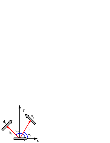
Figure 2: Geometry and parameters of a trimer aggregate. One monomer is chosen to be positioned at the origin of the coordinate system, with the transition dipole moment pointing along the $x$ axis. The positions the transition dipole moments of the other two molecules in space are characterized by their distance $h_{2}$ and $h_{3}$ from the origin of coordinates and by the angles $\alpha_{2}$ and $\alpha_{3}$. Orientations and lengths of the dipoles are given in Tab. 1. In our example we assume that the aggregate is planar.

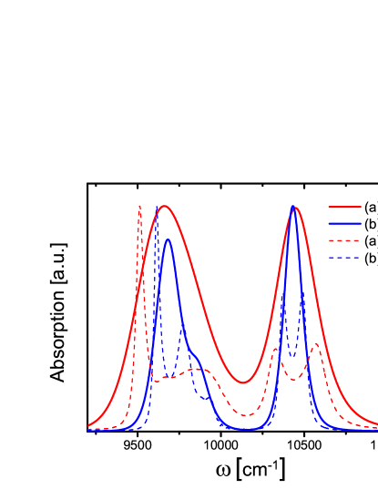
Figure 3: Linear absorption spectrum of the model trimer for various parameters of the system bath interaction: (a) $\lambda=120$ cm^-1, $\tau_{c}=50$ fs, (b) $\lambda=30$ cm^-1 , $\tau_{c}=100$ fs, calculated by the secular TL theory (full lines) and the secular TNL theory (dashed lines).

V.1 Population relaxation and evolution of coherences

First, we compare relaxation dynamics of populations of excited state of our aggregate after excitation by an ultrashort laser pulse. TL equations of motion where solved by standard numerical methods for ordinary differential equations provided by the Mathematica^® software. For the TNL equations we used fast Fourier transform method. Figure 4 presents the first $1$ ps of the population dynamics after a $\delta-$pulse excitation of the trimer from Tab. 1 at the temperature ${\cal T}=300$ K. Reorganization energy $\lambda=120$ cm^-1 and correlation time $\tau_{c}=50$ fs are the same at all three monomers. The dynamics with the same parameters for a selected coherences element $\rho_{13}(t)$ is presented in Fig. 5. The overall conclusion is that all four methods yield a similar general behavior for the populations, with some difference at the short time evolution and also slightly different long time equilibrium. Examination of the Figure 5 leads us to the conclusion that the methods yield two different results - a short coherence life time for the time local methods, and a relatively longer life time in case of the time non-local methods. The behavior of the coherence $\rho_{13}(t)$ represents a general tendency that we have observed for all electronic coherences over a wide range of parameters.

Let us now concentrate on short time behavior of the populations and coherences in more retail. In the short time evolution of the coherences the four methods group into two distinct groups with short (TL methods) and long (TNL methods) coherence life time. Whether the underlying equation is secular or not seems to have only a little influence on the coherence dynamics. Fig. 6 shows the short time ($0-400$ fs) comparison of the population calculated by the four equations of motion. We can clearly see that the results can be naturally grouped according to the presence of fast oscillatory modulation of the population relaxation dynamics. In the one group we have the full TL and full TNL methods, where such oscillations clearly occur, the second group comprises the two secular methods with no oscillations present. Thus, it can be concluded that the non-secular terms in the equations of motion are the cause of these oscillations. This is also supported by comparison of the population dynamics of the full TL and full TNL equations from Fig. 4 (e.g. the population of the state $1$). The oscillation on the full TNL curve last longer than those of the full TL one, which reflects the longer coherence life time we have found for the TNL equations.

Let us now discuss the long time limit of the time evolution. As expected, the two secular theories yield the same equilibrium at long population times. This equilibrium corresponds to the canonical distribution of population among the excitonic levels at ${\cal T}=300$ K. In both secular TNL and secular TL cases, coherences have relaxed to zero at long times as the inset of the Fig. 5 demonstrates. The non-secular TNL and TL equations yield non-zero, stationary coherences at long times, and correspondingly, the long time equilibrium populations do not correspond to the canonical thermal equilibrium. Although both non-secular theories converge to results different from the canonical equilibrium, the full TNL equation yields populations that are physical at all times for the studied system parameters, i.e. they are always positive. The full TL equation on the other hand fails to keep probabilities positive at long times, and the occupation probability of the highest electronic level becomes negative after $200$ fs for the parameters used on Fig. 4.

In light of recent experiments EngelNature , the conclusion that time non-local theories lead to a longer coherence life time than the time-local ones (i.e. also longer than the standard constant rate theories) is probably the most interesting. We have performed calculations of the RDM dynamics while varying the reorganization energy and the correlation time. The absolute values of the coherence $\rho_{13}(t)$ elements were fitted by a single exponential to estimate coherence life-time. The results are summarized in Fig. 7. The Fig. 7A shows the results for secular TL and secular TNL equations. Clearly, with growing correlation time $\tau_{c}$, the full TNL equations lead to a increasing coherence life time. The full TL equation shows only a very weak dependence of the coherence life time on correlation time. Another interesting observation is that for correlation time longer then $50$ fs, the dependence of the coherence life time on the reorganization energy $\lambda$ is different for full TNL and TL methods. Time local theory, in accordance with the standard rate theories, predicts decrease of the coherence life time with $\lambda$. The full TNL theory predicts (within the parameter range studied here) an opposite tendency. The Fig. 7B shows similar conclusion for the non-secular versions of the theories, with the same difference between TL and TNL theory. The dependence of the coherence life time on $\lambda$ in case of TNL equations is not monotonous.

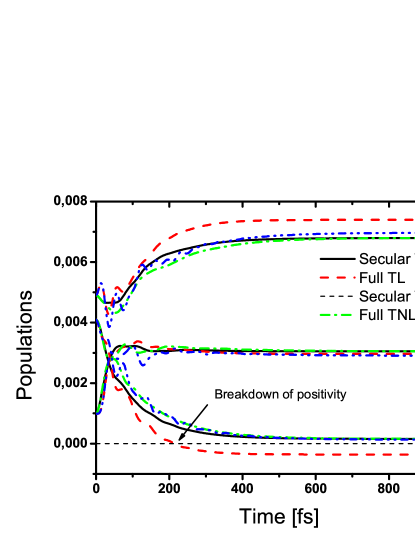
Figure 4: First 1000 fs of the excited state population dynamics of a trimer with parameters $\lambda=120$ cm^-1, $\tau_{c}=50$ fs, calculated by all four methods. For these particular parameters, the full TL equation breaks positivity of the RDM diagonal elements after $200$ fs. Its prediction for the populations of the lowest and highest levels is significantly different from the other three methods.

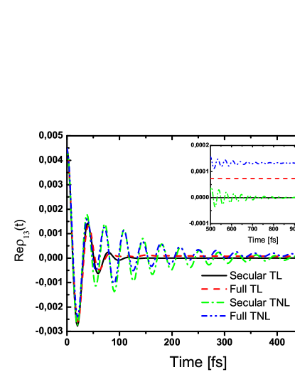
Figure 5: First 500 fs of the dynamics of the RDM coherence element $\rho_{13}(t)$, with parameters from Fig. 4, calculated by all four methods. Detail of the long time part of the time evolution is presented in the inset.

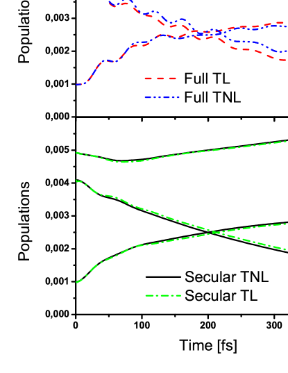
Figure 6: First $400$ fs of the population dynamics of the trimer with parameters $\lambda=30$ fs and $\tau_{c}=100$ fs. Results of full TL and TNL theories are presented in upper subfigure (A), the secular results are found the the lower subfigure (B).

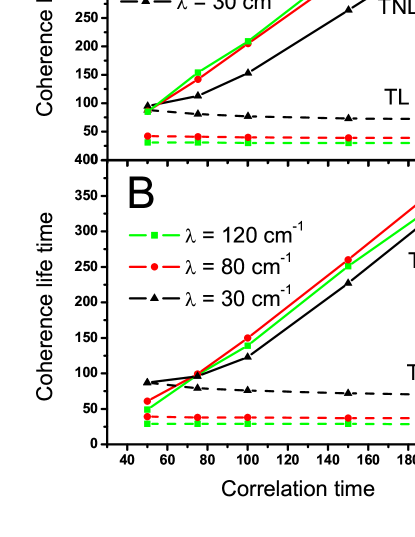
Figure 7: The life time of coherence $\rho_{13}(t)$ as obtained from fitting the coherence dynamics calculated by all four methods for various parameters $\lambda$ and $\tau_{c}$. The upper subfigure (A) shows the life times obtained by the secular methods, while the lower subfigure (B) presents the same for non-secular methods.

V.2 Two-dimensional spectrum

As discussed in the Introduction, the secular TL equation of motion yields an exact result for the dephasing of an isolated optical coherence Haenggi08 . One can show, by comparison of the absorption spectra calculated by secular TL and TNL methods (see Fig. 3), that the TNL theory leads to certain artifacts (second peak) and is therefore not suitable for the description of the optical coherence evolution. Consequently, on can only hope to obtain valid results for the evolution superoperators at the first and the third time interval of the third order response functions by the TL theories. In Ref. Mancal04a it was shown that non-secular terms in the TL equations for optical coherences lead to temperature dependence of the positions of excitonic bands in absorption spectra. This dependence was shown to be strong when the electronic states involved are characterized by significantly different reorganization energy Mancal04a ; Mancal08a . Indeed it can be shown for homodimer that the non-secular terms are exactly zero in second order TL theory if the monomers exhibit the same reorganization energy Mancal08a . We can therefore expect the non-secular effects in the optical coherences to be weak in our case, and we choose secular TL to calculate the evolution superoperators in the first and third time interval of the response function, Eq. (40).

Concerning the population interval, the situation is somewhat different. As we have shown above, the non-secular TL theory leads to dynamics that breaks the positivity condition for the population probabilities at long times. At the same time, short time dynamics is very similar to the full TNL. Both theories predict population oscillations during the life time of the electronic coherences. The full TNL equation, however, preserves positivity, at least for the parameters studied here, and can be therefore used to calculate meaningful 2D spectra. For the same reason, both secular theories can also be successfully used to calculate 2D spectrum. As the oscillation of the populations predicted by non-secular theories are too small to be reliably observed in 2D spectrum (only a small change of the crosspeak amplitude due to the population transfer is observed after $140$ fs of relaxation in 2D spectrum of Fig. 8 ) we expect only a small difference of the 2D spectrum to appear between the secular and full TNL theories. For the calculation of the representative 2D spectrum we therefore choose the secular TL and the full TNL theories. These two differ from each other mainly in the prediction of the life time of the electronic coherences. The observable difference in the calculated 2D spectra should therefore predominantly result from the different life time of the electronic coherence.

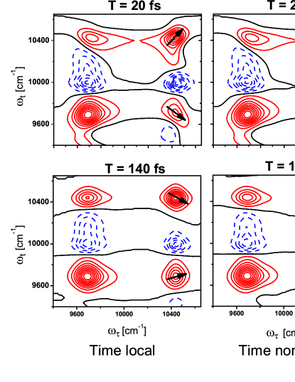
Figure 8: Two-dimensional coherent spectra of the trimer model at population times $T=0$, $20$ and $140$ fs calculated by the secular TL method (left column) and the full TNL method (right column). The system-bath interaction parameters are $\lambda=30$ cm^-1 and $\tau_{c}=100$ fs. The coherence element $\rho_{13}(t)$, which is mainly responsible for the oscillatory behavior of the crosspeaks, is presented in the upper right corner of the figure. The 2D spectrum at $T=0$ fs is the same for both methods and is therefore presented only once. The population times are selected so that they represent different phases of the $\rho_{13}(t)$ element (denoted by arrows on the coherence element figure). Arrows in the 2D spectra denote the orientation of the peaks. All spectra are normalized to 1 with contour step of $10$ %. Positive features are in full red line, negative features are represented by dashed blue line, and the zero contour is depicted by the full black line.

Fig. 8 presents 2D spectra for $\lambda=30$ cm^-1 and $\tau_{c}=100$ fs. These parameters lead to a rather slow relaxation and consequently to narrow spectral peaks in both absorption (see Fig. 3) and 2D spectra. This allows us to clearly see characteristic $T-$dependent oscillations of the peaks in 2D spectrum. At $T=0$ fs, both methods provide the same 2D spectrum, with four peaks. Two diagonal peaks arise when all three perturbations of the system by electric field occur on the same level, while two crosspeaks appear from interactions occurring on different levels. Negative peaks correspond to excited state absorption (see Fig. 1). For two molecules that are not excitonically coupled, all contributions to the crosspeaks cancel out exactly, while if two molecules are excitonically coupled non-zero crosspeaks appear. The shapes of the peaks are influenced by the phase evolution of the coherence elements of RDM during the population time $T$. On the upper left figure of Fig. 8 we have marked the elongation of the diagonal and off-diagonal peaks by arrows. The elongation can be best judged by looking at the zero contour (in black). This particular elongation is characteristic for the phase of the $\rho_{13}(t)$ element (see upper right figure of Fig. 8) at $T=0$. At $T=20$ fs the phases of the $\rho_{13}(t)$ calculated by both methods are opposite to the phase at $T=0$. The 2D spectra calculated by the two different methods at $T=20$ fs differ only in the precise positions of the contours. This phase of the coherence element is characterized in 2D spectrum by a different orientation of the peaks. Interestingly, at $T=140$ fs the two methods predict $\rho_{13}(t)$ that have mutually opposite phases and as a consequence the 2D spectra at $T=140$ fs calculated by different methods differ in the orientation of their crosspeaks. Since the secular TL theory predicts a simple dephasing of the coherence and a regular oscillation with a single frequency proportional to the energy difference between corresponding energy levels, it is in principle possible to distinguish, even experimentally, deviations from this prediction. Our conclusion is that such a deviation should be a consequence of the memory effects in the reduced system time evolution.

V.3 Validity of secular and Markov approximations

Several conclusions about the applicability of the secular and Markov approximations can be drawn from the above results. As pointed out in Ref. Haenggi08 , Markov approximation, which in the second order in system-bath coupling converts the TNL equations to the TL ones, leads accidentally to an exact result for an optical coherence element interacting with the harmonic bath. It has been also pointed out previously Ishizaki2 ; Kubo69 that in the same case, the TNL equations lead to artifacts. When studying relaxation dynamics of the populations and electronic coherences in excitonic systems, full TL theory leads to a breakdown of the positivity of the RDM, while none of the secular theories suffer from this problem. In principle, the full TNL theory suffers from this problem, too. However, it has been found less susceptible to it here. The secular theories lead to canonical density matrix at long times, while the full TNL results in a stationary state characterized by non-zero (but constant) coherences. Such result corresponds to an additional renormalization of the electronic states by the interaction with bath, and has to be expected even at a weak coupling limit Tannor00 . It is important to note in this context that the canonical equilibrium is to be expected for the system consisting of the molecule and the bath as a whole, not for its parts Tannor00 .

For the population dynamics we are therefore forced to conclude that the full TNL theory represents the best candidate for a correct description of relaxation phenomena in the second order of the system bath interaction. It predicts similar population transfer times as other methods, it is much less sensitive to the breakdown of the positivity than its TL counterpart, and it leads to a bath renormalization of the canonical equilibrium. Most interestingly however, it predicts longer coherence life time than the TL theory. It was recently established by Ishizaki and Fleming Ishizaki2 that this is to be expected from a higher order theory.

In the light of the above conclusions about the dynamics of optical coherences and the populations and coherences of the one exciton band, we suggest a hybrid approach to calculating 2D spectra, which consists of the application of the TL method on optical coherences (first and third time interval) and the full TNL method on the calculation of the RDM dynamics in the one exciton band during the population time $T$.

VI Conclusions

In this paper we have compared four different theories of excitation energy transfer and relaxation in molecular aggregate systems, with a special attention paid to lifetime of electronic coherences. Second order time non-local and time local theories with and without secular approximation were studied. For our specific model of an aggregate we have concluded that time non-local theories can account for experimentally observed electronic coherence life time that is significantly longer than the one predicted by the standard time-local secular relaxation rate theory. Markov approximation leading to time local equations of motion was found to be responsible for the reduction of the coherence lifetime, while the influence of the secular approximation on the life time was found rather weak. The time local theory without secular approximation is found to break positivity of the occupation probabilities in the range of parameters studied here. We conclude that time-local second order theory is not suitable for simulating the coherence transfer effects. Simulations of two-dimensional spectra show that the time non-local effects can be experimentally identified based on the analysis of the oscillations of the cross peaks.

Appendix A Third Order Response Functions

In this appendix we list the third order response function used in calculating the impulsive 2D spectra. The first index of the response function follows the standard notation of Ref. MukamelBook . The second index is $g$ for pathways not involving the two-exciton band, while all pathways denoted by $f$ include a two-exciton contribution (see e.g. Ref. BrixnerMancal ).

$$R_{1g}(t,T,\tau)=tr\{\mu_{ge}{\cal U}_{egeg}(t){\cal V}_{eg}^{(R)}$$

$$\times{\cal U}_{eeee}(T){\cal V}_{ge}^{(R)}{\cal U}_{egeg}(\tau){\cal V}_{eg}^{(L)}\rho_{0}\},$$ (46)

$$R_{2g}(t,T,\tau)=tr\{\mu_{ge}{\cal U}_{egeg}(t){\cal{\cal V}}_{eg}^{(R)}$$

$$\times{\cal U}_{eeee}(T){\cal V}_{eg}^{(L)}{\cal U}_{gege}(\tau){\cal V}_{ge}^{(R)}\rho_{0}\},$$ (47)

$$R_{3g}(t,T,\tau)=tr\{\mu_{ge}{\cal U}_{egeg}(t){\cal V}_{eg}^{(L)}$$

$$\times{\cal U}_{gggg}(T){\cal V}_{eg}^{(R)}{\cal U}_{gege}(\tau){\cal V}_{ge}^{(R)}\rho_{0}\},$$ (48)

$$R_{4g}(t,T,\tau)=tr\{\mu_{ge}{\cal U}_{egeg}(t){\cal V}_{eg}^{(L)}$$

$$\times{\cal U}_{gggg}(T){\cal V}_{ge}^{(L)}{\cal U}_{egeg}(\tau){\cal V}_{eg}^{(L)}\rho_{0}\},$$ (49)

$$R_{1f}(t,T,\tau)=tr\{\mu_{fe}{\cal U}_{efef}(t){\cal V}_{ef}^{(R)}$$

$$\times{\cal U}_{eeee}(T){\cal V}_{ge}^{(R)}{\cal U}_{egeg}(\tau){\cal V}_{eg}^{(L)}\rho_{0}\}$$ (50)

$$R_{2f}(t,T,\tau)=tr\{\mu_{fe}{\cal U}_{efef}(t){\cal V}_{ef}^{(R)}$$

$$\times{\cal U}_{eeee}(T){\cal V}_{eg}^{(L)}{\cal U}_{gege}(\tau){\cal V}_{ge}^{(R)}\rho_{0}\}.$$ (51)

Operators and superoperators used in this appendix are defined in Section IV.1.

References

- (1) Quantum Dynamics of Complex Molecular Systems, edited by D. A. Micha and I. Burghardt (Springer, Berlin, 2007).
- (2) H. van Amerongen, R. van Grondelle, and L. Valkunas, Photosynthetic Excitons (Kluwer Academic Publishers, Dordrecht, 2000).
- (3) S. Mukamel, Principles of nonlinear spectroscopy (Oxford University Press, Oxford, 1995).
- (4) T. Renger and R. A. Marcus, J. Chem. Phys. 116, 9997 (2002).
- (5) B. P. Krueger, G. D. Scholes, and G. R. Fleming, J. Phys. Chem. B 102, 5378 (1998).
- (6) M. E. Madjet, A. Abdurahman, and T. Renger, J. Phys. Chem. B 110, 17268 (2006).
- (7) A. Damjanovic, I. Kosztin, U. Kleinekathöfer, and K. Schulten, Phys. Rev. E 65, 031919 (2002).
- (8) D. M. Jonas, Annu Rev. Phys. Chem 54, 425 (2003).
- (9) M. L. Cowan, J. P. Ogilvie, and R. J. D. Miller, Chem. Phys. Lett. 386, 184 (2004).
- (10) T. Brixner, I. V. Stiopkin, and G. R. Fleming, Opt. Lett. 29, 884 (2004).
- (11) T. Brixner, T. Mančal, I. V. Stiopkin, and G. R. Fleming, J. Chem. Phys. 121, 4221 (2004).
- (12) A. V. Pisliakov, T. Mančal, and G. R. Fleming, J. Chem. Phys. 124, 234505 (2004).
- (13) P. Kjellberg, B. Brüggemann, and T. Pullerits, Phys. Rev. B 74, 024303 (2006).
- (14) G. S. Engel, T. R. Calhoun, E. L. Read, T. K. Ahn, T. Mančal, Y.-C. Cheng, R. E. Blankenship, and G. R. Fleming, Nature 446, 782 (2007).
- (15) H. Lee, Y.-C. Cheng, and G. R. Fleming, Science 316, 1462 (2007).
- (16) E. Collini and G. D. Scholes, Science 323, 369 (2009).
- (17) P. Rebentrost, M. Mohseni, I. Kassal, S. Lloyd, and A. Aspuru-Guzik, New J. Phys. 11, 033003 (2009).
- (18) M. Mohseni, P. Rebentrost, S. Lloyd, and A. Aspuru-Guzik, J. Chem. Phys. 129, 174106 (2008).
- (19) M. Plenio and S. F. Huelga, New J. Phys. 10, 113019 (2008).
- (20) A. Olaya-Castro, C. F. Lee, F. F. Olsen, and N. F. Johnson, Phys. Rev. B 78, 085115 (2008).
- (21) S. Nakajima, Progr. Theor. Phys. 20, 948 (1958).
- (22) R. Zwanzig, Physica 30, 1109 (1964).
- (23) N. Hashitsume, F. Shibata, and M. Shingu, J. Stat. Phys. 17, 155 (1977).
- (24) F. Shibata, Y. Takahashi, and N. Hashitsume, J. Stat. Phys. 17, 171 (1977).
- (25) S. Mukamel, I. Oppenheim, and J. Ross, Phys. Rev. A 17, 1988 (1978).
- (26) S. Mukamel, Chem. Phys. 37, 33 (1979).
- (27) V. May and O. Kühn, Charge and Energy Transfer Dynamics in Molecular Systems (Kluwer Academic Publishers, Dordrecht, 2000).
- (28) V. Čápek, I. Barvík, and P. Heřman, J. Luminiscence 204, 306 (2004).
- (29) W. M. Zhang, T. Meier, V. Chernyak, and S. Mukamel, J. Chem. Phys. 108, 7763 (1998).
- (30) M. N. Yang and G. R. Fleming, Chem. Phys. 275, 355 (2002).
- (31) S. J. Jang, M. D. Newton, and R. J. Silbey, Phys. Rev. Lett. 92, 218301 (2004).
- (32) A. Ishizaki and G. R. Fleming, J. Chem. Phys. 130, 243110 (2009).
- (33) A. Ishizaki and G. R. Fleming, J. Chem. Phys. 130, 243111 (2009).
- (34) T. Mančal, L. Valkunas, and G. R. Fleming, Spectroscopy 204, 306 (2008).
- (35) R. Doll, D. Zueco, M. Wubs, S. Kohler, and P. Hanggi, Chem. Phys. 347, 243 (2008).
- (36) B. Fain, Irreversibilities in Quantum Mechanics (Kluwer Academic Publishers, Dordrecht, 2000).
- (37) G. Lindblad, Commun. Math. Phys. 48, 119 (1976).
- (38) D. Zigmantas, E. L. Read, T. Mancal, T. Brixner, A. T. Gardiner, R. J. Cogdell, and G. R. Fleming, Proc. Nat. Acad. Sci. USA 103, 12672 (2006).
- (39) M. H. Cho, H. M. Waswani, T. Brixner, J. Stenger, and G. R. Fleming, J. Phys. Chem. B 109, 10542 (2005).
- (40) T. Mančal, L. Valkunas, and G. R. Fleming, Chem. Phys. Lett. 432, 301 (2006).
- (41) R. Kubo, Adv. Chem. Phys. 15, 11 (1969).
- (42) E. Geva, E. Roseman, and D. Tannor, J. Chem. Phys. 113, 1380 (2000).