Percolation Thresholds of the Fortuin-Kasteleyn Cluster for a Potts Gauge Glass Model on Complex Networks

Abstract

It was pointed out by de Arcangelis et al. [Europhys. Lett. 14 (1991), 515] that the correct understanding of the percolation phenomenon of the Fortuin-Kasteleyn cluster in the Edwards-Anderson model is important since a dynamical transition, which is characterized by a parameter called the Hamming distance or damage, and the percolation transition are related to a transition for a signal propagating between spins. We show analytically the percolation thresholds of the Fortuin-Kasteleyn cluster for a Potts gauge glass model, which is an extended model of the Edwards-Anderson model, on random graphs with arbitary degree distributions. The results are shown on the Nishimori line. We also show the results for the infinite-range model.

1 Introduction

The study of spin models on complex networks has been carried out [1, 2, 3]. We study a spin model on random graphs with arbitary degree distributions as an example of the study of a spin model on complex networks. The behavior of spins on a no growing network is investigated.

We investigate a Potts gauge glass model [4] as a spin model. The Potts gauge glass model is a spin-glass model and is an extended model of the Edwards-Anderson model [5] which is known as a spin-glass model. The understanding of the Edwards-Anderson model on random graphs and on the Bethe lattice is still incompleted [1, 6, 7]. The understanding of the Potts gauge glass model on random graphs and on the Bethe lattice is also incompleted.

The Nishimori line [4] is a line on the phase diagram for the exchange interactions and the temperature. The internal energy and the upper bound of the specific heat are exactly calculated on the Nishimori line [4]. The location of the multicritical point on the square lattice was conjectured, and it was shown that the conjectured value is in good agreement with the other numerical estimates [8]. We will obtain results on the Nishimori line.

There is a case where a percolation transition of networks occures. A network is divided into many networks by deleting some of its nodes and/or links. There is also a case where a percolation transition of clusters occurs. A cluster consists of fictitious bonds. The bond is put between spins. One of the clusters becomes a giant component when a cluster is percolated. We discuss the percolation transition of a cluster.

We investigate the percolation transition of the Fortuin-Kasteleyn (FK) cluster in the FK random cluster model [9, 10]. In the ferromagnetic spin model, the percolation transition point of the FK cluster agrees with the phase transition point. For example, the agreement in the ferromagnetic Ising model is described in Ref. CK. On the other hand, in the Edwards-Anderson model that has a conflict in the interactions, the percolation transition point of the FK cluster disagrees with the phase transition point. It was pointed out by de Arcangelis et al. that, despite the disagreement, the correct understanding of the percolation phenomenon of the FK cluster in the Edwards-Anderson model is important since a dynamical transition, which is characterized by a parameter called the Hamming distance or damage, is occurred at a temperature very close to the percolation temperature, and the dynamical transition and the percolation transition are related to a transition for a signal propagating between spins [12]. We analytically obtain the percolation thresholds of the FK cluster for the Potts gauge glass model.

We use a gauge transformation for deriving results. The gauge transformation was proposed in Ref. NS. In addition to the application of the gauge transformation, results are shown by applying a criterion [13] for spin models on the random graphs with arbitary degree distributions.

In Ref. Y, by applying the criterion with a gauge transformation, the percolation thresholds of the FK cluster for the Edwards-Anderson model on the random graphs with arbitary degree distributions were analytically calculated on the Nishimori line.

We also show the results for the infinite-range model.

This article is organized as follows. First in §2, a complex network model and the Potts gauge glass model are described. The FK cluster is described in §3 and appendix. A criterion for percolation of cluster is explained in §4. We will find in §5 the percolation thresholds. This article is summarized in §6.

2 A complex network model and a Potts gauge glass model

A network consists of nodes and links. A link connected between nodes. The complex network model that we investigate is random graphs with arbitary degree distributions. The networks have no correlation between nodes. The node degree, $k$, is given with a distribution $p(k)$. The links are randomly connected between nodes.

We define a variable $b(i,j)$, where $b(i,j)$ gives one when nodes $i$ and $j$ is connected by a link. $b(i,j)$ gives zero when nodes $i$ and $j$ are not connected by the link. The degree $k(i)$ of node $i$ is given by

$$k(i)=\sum_{j}b(i,j)\,.$$ (1)

The coordination number (the average of the node degree for links), $\langle k\rangle_{N}$, is given by

$$\langle k\rangle_{N}=\frac{1}{N}\sum_{i}^{N}k(i)\,,$$ (2)

where $\langle\,\rangle_{N}$ is the average over the entire network. $N$ is the number of nodes. The average of the square of the node degree for links, $\langle k^{2}\rangle_{N}$, is given by

$$\langle k^{2}\rangle_{N}=\frac{1}{N}\sum_{i}^{N}k^{2}(i)\,.$$ (3)

We define

$$a=\frac{2\langle k\rangle_{N}}{\langle k^{2}\rangle_{N}}\,,$$ (4)

where $a$ represents an aspect of the network.

Figure 1: Relation between the aspect $a$ and the model on the network.

Figure 1 shows the relation between the aspect $a$ and the model on the network. The network is almost a complete graph when $a$ is close to zero, and the model on the network is almost an infinite-range model. The model on the network is the infinite-range model when $\langle k\rangle_{N}=N-1$, $\langle k^{2}\rangle_{N}=(N-1)^{2}$, and $a=2/(N-1)$. The network consists of many cycle graphs when $a$ is one and $\langle k\rangle_{N}$ is two. The model on the network consists of many chain models when $a$ is one and $\langle k\rangle_{N}$ is two. In the Erdős-Rényi (ER) random graph model and in the Gilbert model, the distribution of node degree is the Poisson distribution [1]. The ER random graph model is a network model wherein the network consists of a fixed number of nodes and a fixed number of links, and the links are randomly connected between the nodes. The Gilber model is a network model wherein the link between nodes is connected with a given probability. In the ER random graph model and in the Gilbert model, $\langle k^{2}\rangle_{N}=\langle k\rangle_{N}(\langle k\rangle_{N}+1)$, and $a=2/(\langle k\rangle_{N}+1)$.

The Hamiltonian for a Potts gauge glass model, ${\cal H}$, is given by [4]

$${\cal H}=-\frac{J}{2q}\sum^{N}_{i}\sum_{\{j|b(i,j)=1\}}\sum_{r_{i,j}=1}^{q-1}e^{\frac{2\pi i}{q}(\nu_{i,j}+q_{i}-q_{j})r_{i,j}}\,,$$ (5)

where $q_{i}$ denotes the state of the spin on node $i$, and $q_{i}=0,1,\ldots,q-1$. $\nu_{i,j}$ denotes a variable related to the strength of the exchange interaction between the spins on nodes $i$ and $j$, and $\nu_{i,j}=0,1,\ldots,q-1$. $q$ is the total number of states that a spin takes.

We use representations: $\lambda_{i}=e^{\frac{2\pi i}{q}q_{i}}$ and $J^{(r_{i,j})}_{i,j}=Je^{\frac{2\pi i}{q}\nu_{i,j}r_{i,j}}$. Then, the Hamiltonian (Eq. (5)) is given by

$${\cal H}=-\frac{1}{2q}\sum^{N}_{i}\sum_{\{j|b(i,j)=1\}}\sum_{r_{i,j}=1}^{q-1}J^{(r_{i,j})}_{i,j}\lambda^{r_{i,j}}_{i}\lambda^{q-r_{i,j}}_{j}\,.$$ (6)

The value of $\nu_{i,j}$ is given with a distribution $P(\nu_{i,j})$. The distribution $P(\nu_{i,j})$ is given by

$$P(\nu_{i,j})=p\,\delta_{\nu_{i,j},0}+\frac{1-p}{q-1}(1-\delta_{\nu_{i,j},0})\,,$$ (7)

where $p$ is the probability that the exchange interaction between the spins is ferromagnetic. $\delta$ is the Kronecker delta. The normalization of $P(\nu_{i,j})$ is given by

$$\sum^{q-1}_{\nu_{i,j}=0}P(\nu_{i,j})=1\,.$$ (8)

When $\nu_{i,j}=0$ ($J^{(r_{i,j})}_{i,j}=J$) for all $(i,j)$ pairs, the model becomes the ferromagnetic Potts model. When $q=2$, the model becomes the Edwards-Anderson model and is especially called the $\pm J$ Ising model.

In Ref. T, it was pointed out that a gauge transformation has no effect on thermodynamic quantities. To calculating thermodynamic quantities, a gauge transformation wherein the transformation is performed by

$$J^{(r_{i,j})}_{i,j}\to J^{(r_{i,j})}_{i,j}\mu^{q-r_{i,j}}_{i}\mu^{r_{i,j}}_{j}\,,\quad\lambda_{i}\to\lambda_{i}\mu_{i}$$ (9)

is used, where $\mu_{i}=e^{\frac{2\pi i}{q}\tilde{q}_{i}}$, and $\tilde{q}_{i}$ is an arbitary valuve for $q_{i}$. This gauge transformation was proposed in Ref. NS. By the gauge transformation, the Hamiltonian ${\cal H}$ part becomes ${\cal H}\to{\cal H}$.

By using Eqs. (7), (8), and (10), the distribution $P(\nu_{i,j})$ is given by [4]

$$P(\nu_{i,j})=Ae^{\frac{\beta_{\rm P}}{q}\sum_{r_{i,j}=1}^{q-1}J^{(r_{i,j})}_{ij}(\nu_{i,j})}\,,$$ (10)

where $A$ and $\beta_{P}$ are respectively

$$A = \frac{1}{e^{\frac{\beta_{P}J}{q}(q-1)}+(q-1)e^{-\frac{\beta_{P}J}{q}}}\,,$$ (11)

$$\beta_{P} = \frac{1}{J}\ln\biggl{[}p\biggl{(}\frac{q-1}{1-p}\biggr{)}\biggr{]}\,.$$ (12)

By performing the gauge transformation, the distribution $P(\nu_{i,j})$ part becomes

$$\prod_{\langle i,j\rangle}P(\nu_{i,j}) = Ae^{\frac{\beta_{\rm P}}{q}\sum_{\langle i,j\rangle}\sum_{r_{i,j}=1}^{q-1}J^{(r_{i,j})}_{i,j}(\nu_{i,j})}$$ (13)

$$\to \frac{A}{q^{N}}\sum_{\{\mu_{i}\}}e^{\frac{\beta_{\rm P}}{q}\sum_{\langle i,j\rangle}\sum_{r_{i,j}=1}^{q-1}J^{(r_{i,j})}_{i,j}(\nu_{i,j})\mu^{q-r_{i,j}}_{i}\mu^{r_{i,j}}_{j}}\,,$$

where $\langle x,y\rangle$ denotes the nearest neighbor pairs conneced by links.

3 The Fortuin-Kasteleyn cluster

The bond for the FK cluster is put between spins with probability $P_{\rm FK}(q_{i},q_{j},\nu_{i,j})$. The value of $P_{\rm FK}$ depends on the interaction between spins and the states of spins. We call the bond the FK bond in this article. $P_{\rm FK}(q_{i},q_{j},\nu_{i,j})$ is given by

$$P_{\rm FK}(q_{i},q_{j},\nu_{i,j})=1-e^{-\frac{\beta}{q}[\sum_{r_{i,j}=1}^{q-1}J^{(r_{i,j})}_{i,j}(\nu_{i,j})\lambda^{r_{i,j}}_{i}(q_{i})\lambda^{q-r_{i,j}}_{j}(q_{j})+J]}\,,$$ (14)

where $\beta$ is the inverse temperature, and $\beta=1/k_{B}T$. $k_{B}$ is the Boltzmann constant, and $T$ is the temperature. By connecting the FK bonds, the FK clusters are generated. In appendix, we will derive Eq. (14). By the gauge transformation, the $P_{\rm FK}$ part becomes $P_{\rm FK}\to P_{\rm FK}$.

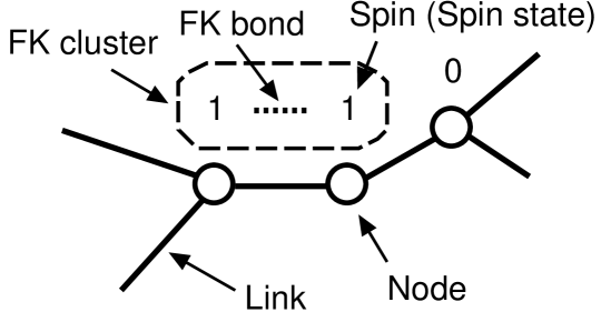
Figure 2: Network and FK cluster. Three nodes, six links, three spins, an FK bond, and an FK cluster are depicted. Spins are aligned on each node and are represented by spin states. In this picture, the states of two spins are one and the state of a spin is zero.

Figure 2 shows a conceptual diagram of a network and an FK cluster. Three nodes, six links, three spins, an FK bond, and an FK cluster are depicted. Spins are aligned on each node and are represented by spin states.

The thermodynamic quantity of the FK bond put between the spins on nodes $i$ and $j$, $[\langle b_{\rm FK}(i,j)\rangle_{T}]_{R}$, is given by

$$[\langle b_{\rm FK}(i,j)\rangle_{T}]_{R}=[\langle P_{\rm FK}(q_{i},q_{j},\nu_{i,j})\rangle_{T}]_{R}\,,$$ (15)

where $\langle\,\rangle_{T}$ is the thermal average, and $[\,]_{R}$ is the random configuration average. The thermodynamic quantity of the node degree for FK bonds at node $i$, $[\langle k_{\rm FK}(i)\rangle_{T}]_{R}$, is given by

$$[\langle k_{\rm FK}(i)\rangle_{T}]_{R}=[\langle\sum_{\{j|b(i,j)=1\}}P_{\rm FK}(q_{i},q_{j},\nu_{i,j})\rangle_{T}]_{R}\,.$$ (16)

The thermodynamic quantity of the square of the node degree for FK bonds at node $i$, $[\langle k^{2}_{\rm FK}(i)\rangle_{T}]_{R}$, is given by

$$[\langle k^{2}_{\rm FK}(i)\rangle_{T}]_{R}$$ (17)

$$= [\langle\sum_{\{j|b(i,j)=1\}}\sum_{\{l|b(i,l)=1\}}P_{\rm FK}(q_{i},q_{j},\nu_{i,j})P_{\rm FK}(q_{i},q_{l},\nu_{i,l})(1-\delta_{j,l})$$

$$+ \sum_{\{j|b(i,j)=1\}}P_{\rm FK}(q_{i},q_{j},\nu_{i,j})\rangle_{T}]_{R}\,.$$

The thermodynamic quantity of the node degree for FK bonds, $[\langle k_{\rm FK}\rangle_{T}]_{R}$, is given by

$$[\langle k_{\rm FK}\rangle_{T}]_{R}=\frac{1}{N}\sum_{i}^{N}[\langle k_{\rm FK}(i)\rangle_{T}]_{R}\,.$$ (18)

The thermodynamic quantity of the square of the node degree for FK bonds, $[\langle k^{2}_{\rm FK}\rangle_{T}]_{R}$, is given by

$$[\langle k^{2}_{\rm FK}\rangle_{T}]_{R}=\frac{1}{N}\sum_{i}^{N}[\langle k^{2}_{\rm FK}(i)\rangle_{T}]_{R}\,.$$ (19)

4 A criterion for percolation of cluster

We use a conjectured criterion for deriving the percolation thresholds. This criterion is a criterion of the percolation of cluster for spin models on the random graphs with arbitary degree distributions, and is given by [13]

$$[\langle k^{2}_{\rm bond}\rangle_{T}]_{R}\geq 2[\langle k_{\rm bond}\rangle_{T}]_{R}\,,$$ (20)

where $k_{\rm bond}$ is a quantity for a bond put between spins. $k_{\rm bond}$ for the FK bond is $k_{\rm FK}$ for example. Equation (20) is given by the inequality when the cluster is percolated. Equation (20) is given by the equality when the cluster is at the percolation transition point.

In addition, Eq. (20) is true for sufficiently large number of nodes in the case that the magnitude of the bond does not depend on the degree $k(i)$.

We consider the condition that the magnitude of the bond does not depend on the degree $k(i)$. We define a variable for the inverse temperature $\beta$ as $\rho(\beta)$. We set

$$0<\rho(\beta)\leq 1\,.$$ (21)

We consider a case that $[\langle b_{\rm bond}(i,j)\rangle_{T}]_{R}$, $[\langle k_{\rm bond}(i)\rangle_{T}]_{R}$, and $[\langle k^{2}_{\rm bond}(i)\rangle_{T}]_{R}$ are respectively written as

$$[\langle b_{\rm bond}(i,j)\rangle_{T}]_{R}=\rho(\beta)\,,$$ (22)

$$[\langle k_{\rm bond}(i)\rangle_{T}]_{R}=\rho(\beta)\,k(i)\,,$$ (23)

$$[\langle k^{2}_{\rm bond}(i)\rangle_{T}]_{R} = \rho^{2}(\beta)\,k(i)[k(i)-1]$$ (24)

$$+ \rho(\beta)\,k(i)\,.$$

In the case, it is implied that the bias for $k(i)$ does not appear in the statistical results of the bonds. Therefore, we describe the case that $[\langle b_{\rm bond}(i,j)\rangle_{T}]_{R}$, $[\langle k_{\rm bond}(i)\rangle_{T}]_{R}$, and $[\langle k^{2}_{\rm bond}(i)\rangle_{T}]_{R}$ are respectively written as Eqs. (22), (23), and (24) as the case that the magnitude of the bond does not depend on $k(i)$.

This criterion is a conjectured criterion and is not exactly derived yet. On the other hand, it was confirmed [13] that this criterion is exact for several extremal points when applied to the Edward-Anderson model. In this article, we do not examine this criterion and just apply this criterion to the present system.

5 Results

We will obtain the percolation thresholds of the FK cluster in this section.

By using Eqs. (9), (13), (14), and (15), when $\beta=\beta_{P}$, the thermodynamic quantity of the FK bond put between the spins on nodes $i$ and $j$, $[\langle b_{\rm FK}(i,j)\rangle_{T}]_{R}$, is obtained as

$$[\langle b_{\rm FK}(i,j)\rangle_{T}]_{R}$$ (25)

$$= \sum_{\{\nu_{l,m}\}}\prod_{\langle l,m\rangle}P(\nu_{l,m})\frac{\sum_{\{q_{l}\}}P_{\rm FK}(q_{i},q_{j},\nu_{i,j})\,e^{-\beta_{P}{\cal H}(\{q_{l}\},\{\nu_{l,m}\})}}{\sum_{\{q_{l}\}}e^{-\beta_{P}{\cal H}(\{q_{l}\},\{\nu_{l,m}\})}}$$

$$= \frac{A^{N_{B}}}{q^{N}}\sum_{\{\nu_{l,m}\}}\sum_{\{S_{l}\}}P_{\rm FK}(q_{i},q_{j},\nu_{i,j})\,e^{-\beta_{P}{\cal H}(\{q_{l}\},\{\nu_{l,m}\})}$$

$$= \frac{e^{\beta_{P}J}-1}{e^{\beta_{P}J}+q-1}\,,$$

where $N_{B}$ is the number of all links, and $N_{B}=N\langle k\rangle_{N}/2$. By using Eqs. (9), (13), (14), and (16), when $\beta=\beta_{P}$, the thermodynamic quantity of the node degree for FK bonds at node $i$, $[\langle k_{\rm FK}(i)\rangle_{T}]_{R}$, is obtained as

$$[\langle k_{\rm FK}(i)\rangle_{T}]_{R}=\biggl{(}\frac{e^{\beta_{P}J}-1}{e^{\beta_{P}J}+q-1}\biggr{)}\,k(i)\,.$$ (26)

By using Eqs. (9), (13), (14), and (17), when $\beta=\beta_{P}$, the thermodynamic quantity of the square of the node degree for FK bonds at node $i$, $[\langle k^{2}_{\rm FK}(i)\rangle_{T}]_{R}$, is obtained as

$$[\langle k^{2}_{\rm FK}(i)\rangle_{T}]_{R}$$ (27)

$$= \biggl{(}\frac{e^{\beta_{P}J}-1}{e^{\beta_{P}J}+q-1}\biggr{)}^{2}\,k(i)[k(i)-1]$$

$$+ \biggl{(}\frac{e^{\beta_{P}J}-1}{e^{\beta_{P}J}+q-1}\biggr{)}\,k(i)\,.$$

When we set

$$\rho(\beta_{P})=\frac{e^{\beta_{P}J}-1}{e^{\beta_{P}J}+q-1}\,,$$ (28)

Eqs (25), (26), and (27) are respectively formulated as Eqs. (22), (23), and (24). Therefore, the magnitude of the bond does not depend on the $k(i)$. By using Eqs. (18), (19), (20), (26), and (27), we obtain

$$\frac{2(e^{\beta_{P}J}-1)}{2(e^{\beta_{P}J}-1)+q}\geq\frac{2\langle k\rangle_{N}}{\langle k^{2}\rangle_{N}}\,.$$ (29)

Equation (29) is given by the inequality when the cluster is percolated. Equation (29) is given by the equality when the cluster is at the percolation transition point.

From Eqs. (21) and (28), there is the percolation transition point for $0<\beta_{P}\leq\infty$. From Eq. (29), there is the percolation transition point for $0<a\leq 1$. By using Eqs. (12) and (29), the probability $p$ that the interaction is ferromagnetic is obtained as

$$p=\frac{2(1-a)+aq}{(2-a)q}$$ (30)

at the percolation transition point. By using Eqs. (12) and (30), the percolation transition temperature $T_{P}$ is obtained as

$$T_{P}=\frac{J}{k_{B}\ln\biggl{[}\frac{2(1-a)+aq}{2(1-a)}\biggr{]}}\,.$$ (31)

Figure 3: Percolation thresholds of the FK cluster for the Potts gauge glass model. (a) The relation between the aspect $a$ and the probability $p$ is shown. (b) The relation between the aspect $a$ and the percolation transition temperature $T_{P}$ is shown. The solid line shows the result of $q=3$, the dotted line shows the result of $q=10$, and the short-dashed line shows the result of $q=100$. $J/k_{B}$ is set to 1.

Figure 3 shows the percolation thresholds of the FK cluster for the Potts gauge glass model. Figure 3(a) shows the relation between the aspect $a$ and the probability $p$. Eq. (30) is used for showing Fig. 3(a). Figure 3(b) shows the relation between the aspect $a$ and the percolation transition temperature $T_{P}$. Eq. (31) is used for showing Fig. 3(b). The solid line shows the result of $q=3$, the dotted line shows the result of $q=10$, and the short-dashed line shows the result of $q=100$. $J/k_{B}$ is set to $1$.

For the ferromagnetic Potts model on the same network, the phase transition temperature $T^{({\rm Ferro})}_{C}$ is [15]

$$T^{({\rm Ferro})}_{C}=\frac{J}{k_{B}\ln\biggl{[}\frac{2(1-a)+aq}{2(1-a)}\biggr{]}}\,.$$ (32)

$T_{P}$ (Eq. (31)) coincides with $T^{({\rm Ferro})}_{C}$.

The complete graph is considerd as $a\sim 0$. We set $\langle k\rangle_{N}=N-1$, $\langle k^{2}\rangle_{N}=(N-1)^{2}$, $a=2/(N-1)$, and $J\to J/\sqrt{N}$. From the settings, the model on the network becomes the infinite-range model. By using Eq. (30), the probability $p^{({\rm IR})}$ that the interaction is ferromagnetic is obtained as

$$p^{({\rm IR})}=\frac{N-3+q}{(N-2)q}\to\frac{1}{q}$$ (33)

for a sufficiently large number of nodes at the percolation transition point. By using Eq. (31), the percolation transition temperature $T^{({\rm IR})}_{P}$ is obtained as

$$T^{({\rm IR})}_{P}=\frac{J}{k_{B}\sqrt{N}\ln(1+\frac{q}{N-3})}\to\frac{J\sqrt{N}}{k_{B}q}$$ (34)

for a sufficiently large number of nodes.

6 Summary

In this article, the Potts gauge glass model on the random graphs with artibary degree distributions was investigated.

The value of $[\langle b_{\rm FK}(i,j)\rangle_{T}]_{R}$, $[\langle k_{\rm FK}(i)\rangle_{T}]_{R}$, $[\langle k^{2}_{\rm FK}(i)\rangle_{T}]_{R}$, $[\langle k_{\rm FK}\rangle_{T}]_{R}$, and $[\langle k^{2}_{\rm FK}\rangle_{T}]_{R}$ on the Nishimori line were shown. They are quantities for the FK bonds and are exact even on a finite number of nodes.

It is known that the internal energy and the upper bound of the specific heat are exactly calculated on the Nishimori line in the Potts gauge glass model without the dependence of the network (lattice) [4]. In this article, it was realized that, as a property for the Nishimori line, the magnitude of the FK bond does not depend on the degree $k(i)$.

In this article, we showed the percolation thresholds of the FK cluster. It was shown that the percolation transition temperature $T_{P}$ (Eq. (31)) on the Nishimori line for the Potts gauge glass model on the present network coincides with the phase transition temperature $T^{({\rm Ferro})}_{C}$ [15] for the ferromagnetic Potts model on the same network. The percolation thresholds of the FK cluster for the infinite-range model were also shown.

We used a conjectured criterion Eq. (20) to obtain the percolation thresholds. For this criterion, it was confirmed [13] that this criterion is exact for several extremal points when applied to the Edward-Anderson model. Therefore, our entire set of results may be exact.

Appendix: the probabilities for connecting spins

We will derive Eq. (14) according to the method of Kawashima and Gubernatis in Ref. KG. We define the weight of two spins on nodes connected by a link as $w(q_{i},q_{j},\nu_{i,j})$. $w(q_{i},q_{j},\nu_{i,j})$ is given by

$$w(q_{i},q_{j},\nu_{i,j})=\exp\biggl{\{}\frac{\beta J}{q}\sum_{r_{i,j}=1}^{q-1}\exp\biggl{[}\frac{2\pi i}{q}\biggr{(}\nu_{i,j}+q_{i}-q_{j}\biggl{)}r_{i,j}\biggr{]}\biggr{\}}\,.$$ (35)

We define the weight $w$ for $\nu_{i,j}+q_{i}-q_{j}=0$ as $w_{\rm para}$. We obtain

$$w_{\rm para}(q_{i},q_{j},\nu_{i,j})=\exp\biggl{[}\frac{\beta J(q-1)}{q}\biggr{]}\,.$$ (36)

We define the weight $w$ for $\nu_{i,j}+q_{i}-q_{j}\neq 0$ as $w_{\rm anti}$. We obtain

$$w_{\rm anti}(q_{i},q_{j},\nu_{i,j})=\exp\biggl{(}-\frac{\beta J}{q}\biggr{)}\,.$$ (37)

We define the weight of graph for connecting two spins as $w(g_{\rm conn})$. We define the weight of graph for disconnecting two spins as $w(g_{\rm disc})$. We are able to write

$$w_{\rm para}(q_{i},q_{j},\nu_{i,j}) = w(g_{\rm conn})+w(g_{\rm disc})\,,$$ (38)

$$w_{\rm anti}(q_{i},q_{j},\nu_{i,j}) = w(g_{\rm disc})\,.$$ (39)

By using Eqs. (36), (37), (38), and (39), we obtain

$$w(g_{\rm conn}) = \exp\biggl{[}\frac{\beta J(q-1)}{q}\biggr{]}-\exp\biggl{(}-\frac{\beta J}{q}\biggr{)}\,,$$ (40)

$$w(g_{\rm disc}) = \exp\biggl{(}-\frac{\beta J}{q}\biggr{)}\,.$$ (41)

We define the probability of connecting two spins for $\nu_{i,j}+q_{i}-q_{j}=0$ as $P_{\rm para}(g_{\rm conn})$. We define the probability of connecting two spins for $\nu_{i,j}+q_{i}-q_{j}\neq 0$ as $P_{\rm anti}(g_{\rm conn})$. We are able to write

$$P_{\rm para}(g_{\rm conn}) = \frac{w(g_{\rm conn})}{w(g_{\rm conn})+w(g_{\rm disc})}\,,$$ (42)

$$P_{\rm anti}(g_{\rm conn}) = 0\,.$$ (43)

By using Eqs. (40), (41), (42), and (43), we derive Eq. (14).

References

[1]
S. N. Dorogovtsev, A. V. Goltsev and J. F. F. Mendes,
Rev. Mod. Phys. 80 (2008), 1275.
[2]
F. Iglói and L. Turban,
Phys. Rev. E 66 (2002), 036140.
[3]
M. Karsai, J-Ch. Anglès d’Auriac and
F. Iglói,
Phys. Rev. E 76 (2007), 041107.
[4]
H. Nishimori and M. J. Stephen,
Phys. Rev. B 27 (1983), 5644.
[5]
S. F. Edwards and P. W. Anderson, J. of Phys. F 5 (1975), 965.
[6]
L. Viana and A. J. Bray, J. of Phys. C 18 (1985), 3037.
[7]
M. Mézard and G. Parisi, Eur. Phys. J. B 20 (2001), 217.
[8]
H. Nishimori and K. Nemoto,
J. Phys. Soc. Jpn. 71 (2002), 1198.
[9]
P. W. Kasteleyn and C. M. Fortuin, J. Phys. Soc. Jpn. Suppl. 26 (1969), 11.
[10]
C. M. Fortuin and P. W. Kasteleyn,
Physica (Utrecht) 57 (1972), 536.
[11]
A. Coniglio and W. Klein, J. of Phys. A 13 (1980), 2775.
[12]
L. de Arcangelis, A. Coniglio and F. Peruggi,
Europhys. Lett. 14 (1991), 515.
[13]
C. Yamaguchi, Prog. Theor. Phys. 124 (2010), 399.
[14]
G. Toulouse, Commun. Phys. 2 (1977), 115.
[15]
S. N. Dorogovtsev, A. V. Goltsev and J. F. F. Mendes,
Eur. Phys. J. B 38 (2004), 177.
[16]
N. Kawashima and J. E. Gubernatis,
Phys. Rev. E 51 (1995), 1547.