Anomalous Soft Photons in Hadron Production

Abstract

Anomalous soft photons in excess of what is expected from electromagnetic bremsstrahlung have been observed in association with the production of hadrons, mostly mesons, in high-energy $K^{+}p$, $\pi^{+}p$, $\pi^{-}p$, $pp$, and $e^{+}e^{-}$ collisions. We propose a model for the simultaneous production of anomalous soft photons and mesons in quantum field theory, in which the meson production arises from the oscillation of color charge densities of the quarks of the underlying vacuum in the flux tube. As a quark carries both a color charge and an electric charge, the oscillation of the color charge densities will be accompanied by the oscillation of electric charge densities, which will in turn lead to the simultaneous production of soft photons during the meson production process. How the production of these soft photons may explain the anomalous soft photon data will be discussed. Further experimental measurements to test the model will be proposed.

I Introduction

Anomalous soft photons are soft photons in excess of what is expected from electromagnetic bremsstrahlung. They have been observed in conjunction with the production of hadrons, mostly mesons, in $K^{+}p$ Chl84 ; Bot91 , $\pi^{+}p$ Bot91 , $\pi^{-}p$ Ban93 ; Bel97 ; Bel02a , $pp$ collisions Bel02 , and in high-energy $e^{+}$-$e^{-}$ annihilations in $Z^{0}$ hadronic decay DEL06 ; DEL09 ; Per09 . Recent DELPHI measurements on the characteristics of the produced hadrons associated with the anomalous soft photon production provide a wealth of information on the production process DEL06 ; DEL09 ; Per09 ; DEL08 . The main features of the anomalous soft photon phenomenon can be summarized as follows:

1. Anomalous soft photons are produced in association with hadron production at high energies. They are absent when there is no hadron production DEL08 .

2. The anomalous soft photon yield is proportional to the hadron yield.

3. The transverse momenta of the anomalous soft photons are in the region of many tens of MeV/c.

4. The anomalous soft photon yield increases approximately linearly as the number of neutral or charged produced particles increases, but, the yield of anomalous soft photons increases much faster with increasing neutral particle multiplicity than with charged particle multiplicity.

Previously, many different theoretical models have been put forth to explain the anomalous soft photon phenomenon. Reviews of the experimental results and theoretical models have been presented Bal90 ; Lic94 . There are models based on the assumption of a cold quark gluon plasma Van89 , boost-invariant classical flux tube Czy94 , gluon dominance Kok07 , Unruh-Davies effect Dar91 , synchrotron radiation in the stochastic nonperturbative QCD vacuum Nac94 , the classical string fragmentation And83 , closed quark-antiquark loop Sim08 , and ADS/CFT Supersymmetric Yang-Mills theory Hat10 . These different proposed models are useful to indicate that to search for the source of the anomalous soft photons, it is necessary to go beyond the electromagnetic bremsstrahlung process. While the various models may explain some features of the process, the fourth feature listed above from the recent DELPHI observations cannot be explained by all existing models DEL09 ; Per09 ; a complete understanding of the basic origin of the anomalous soft photon is still lacking.

We would like to propose a model for the simultaneous production hadron and anomalous soft photons in the $q$-$\bar{q}$ string-fragmentation in quantum field theory to explain the anomalous soft photon phenomenon. As described by Casher, Kogut, and Suskind Cas74 , the production of mesons in such a theory arises from the oscillation of color charge densities of the quark vacuum in the flux tube when a quark and an antiquark (or a diquark) pull away from each other at high energies. These color charge density oscillations obey the Klein-Gordon equation characterized by the mass of the meson Cas74 ; Bjo73 ; Bjo83 ; Sch62 ; Low71 ; Col75 ; Col76 ; Won91 ; Won94 ; Won09 ; Won09a . Because a quark carries both a color charge and an electric charge, the underlying dynamical motion of the quarks in the vacuum that generate color charge density oscillations will also generate electric charge density oscillations in the flux tube. These color charge density oscillations will lead to the production of photons that are clearly additional to those from the electromagnetic bremsstrahlung process. Thus the oscillation of the quark densities in the vacuum will lead to the simultaneous color and electric charge density oscillations and will subsequently lead to simultaneous and proportional production of mesons and anomalous photons, in agreement with the first two features of the anomalous soft photon phenomenon listed in the beginning of this section.

It is of interest to examine whether the model also leads to results that will be consistent with the remaining features of the anomalous soft photon production phenomenon. For such a purpose, we need to know the properties of these electric charge density oscillations of the quarks in the flux tube. Will the electric charge density oscillations also obey the Klein-Gordon equation characterized by a mass to give rise to stable photons in the flux tube environment? If these photons are stable, what are the magnitudes of their masses and how do the masses depend on the quantum numbers and other physical properties? If they are produced, how are they observed experimentally in four-dimensional space-time?

To answer these questions, we start with quarks interacting with both QCD4 and QED4 interactions in four-dimensional space-time in Section II. We specialize to the case of the flux tube formation for high energy particle production processes under longitudinal dominance and transverse confinement. The system can then be approximately compactified into a QCD2$\times$QED2 system in two-dimensional space-time, with the coupling constants in different space-time dimensions related by the flux tube radius. In Section, III, we examine the non-Abelian bosonization of the QCD2$\times$QED2 system. We find stable QCD2 and QED2 bosons for quarks with two flavors arising from the density oscillations of the quarks in the flux tube. These bosons can be identified as QCD2 mesons and QED2 photons. The boson masses are then expressed as a function of the coupling constants and the quark transverse mass. In Section IV, we estimate the coupling constants and the boson masses for the case of the $Z^{0}$ hadronic decay. As QCD2 mesons and QED2 photons are stable in the flux tube environment, we can infer from the quantum field theory description of the particle production process in Ref. Cas74 that these QCD2 mesons and QED2 photons will be produced simultaneously in $q$-$\bar{q}$ string fragmentation. The present model for the production of anomalous soft photons can also be conveniently called the QED2 photon model. In Section V, we discuss the adiabatic decompactification of produced photons and mesons from two-dimensional space-time to particles in four-dimensional space-time. In Section VI, we investigate how the QED2 model of photon production may explain the experimental anomalous soft photon transverse momentum distributions. In Section VII, we examine the rates of QED2 meson and QED2 photon production and the correlation of the soft photon yield with charge and neutral particle multiplicities. In Section VIII, we suggest future experimental measurements to test the QED2 photon model. In Section IX, we present our conclusions and discussions.

II Flux Tube Environment in High Enegy Particle Production Processes

We wish to investigate the process of soft photon production in association with hadron production, in which the produced hadrons consist mostly of mesons. In the quantum field theory description of meson production process as analogous to the particle production process in quantum electrodynamics in two-dimensions (QED2), mesons that are stable within the theory will be produced along the string, when a quark and an antiquark at the two ends of the string pull apart at high energies Cas74 ; Sch62 ; Low71 ; Col75 ; Col76 . The rapidity distribution of these produced mesons exhibits the property of boost invariance in the limit of infinite energies Cas74 ; Bjo73 ; Bjo83 . For a finite energy system, the boost-invariant solution turns naturally into a rapidity plateau, whose width increases with energy as $\ln(\sqrt{s})$ Won91 ; Won94 .

The $q$-$\bar{q}$ string is an idealization of a flux tube with a transverse profile, which reveals itself as the transverse momentum distribution of the produced particles Gat92 . Experimentally, the presence of a flux tube is evidenced by the limiting average transverse momentum and a rapidity plateau Cas74 ; And83 ; Bjo73 ; Bjo83 ; Won91 ; Won94 ; Won09 ; Won09a ; Gat92 as in high-energy $e^{+}$-$e^{-}$ annihilations Aih88 ; Hof88 ; Pet88 ; Abe99 ; Abr99 and $pp$ collisions Yan08 .

To investigate the simultaneous production of QCD and QED quanta in the flux tube fragmentation, we study quarks interacting with both QCD and QED interactions, in circumstances leading to the formation of the flux tube. It becomes convenient to consider the U$(3)$ group which breaks up into the color SU(3) and the electromagnetic U(1) subgroups. The SU(3) and U(1) subgroups differ in their coupling constants and communicative properties. We introduce the generator $t^{0}$ for the U$(1)$ subgroup,

$$t^{0}=\frac{1}{\sqrt{6}}\left(\begin{matrix}1&0&0\cr 0&1&0\cr 0&0&1\end{matrix}\right),$$ (1)

which adds on to the eight generators of the SU$(3)$ subgroup, $\{t^{1},...t^{8}\}$, to form the nine generators of the U(3) group. They satisfy ${\rm tr}\{t^{\alpha}t^{\beta}\}=\delta^{\alpha\beta}/2{~{}~{}\rm for~{}~{}}\alpha,\beta=0,1,..,8$.

Limiting our consideration to quarks with two light flavors, we examine the QCD4$\times$QED4 system in four-dimensional space-time $x^{\mu}$, with $\mu$=0,1,2,3. The dynamical variables are the quark fields, $\psi_{f}^{a}$, and the U(3) gauge fields, $A_{\nu}$=$A_{\nu}^{\alpha}t^{\alpha}$, where $a$ is the color index with $a$=1,2,3, $f$ is the flavor index with $f$=$u,d$, and $\alpha$ is the U(3) generator index with $\alpha$=0,1,..,8. The coupling constants $g_{f}^{\alpha}$ depend on $\alpha$ and $f$ and are given explicitly by

$$g_{u}^{\{1,..,8\}}=g_{d}^{\{1,..,8\}}=g_{\rm QCD4},{\rm~{}~{}for~{}~{}QCD},$$ (2)

$$g_{u}^{0}=-e_{u}=-Q_{u}e_{\rm QED4},~{}~{}~{}g_{d}^{0}=-e_{d}=-Q_{d}e_{\rm QED4}{\rm~{}~{}for~{}~{}QED},$$ (3)

with $Q_{u}=2/3$, and $Q_{d}=-1/3$. We use the convention of summation over repeated indices, but the summation symbol and indices are occasionally written out explicitly to avoid ambiguities. For brevity of notations, the indices $a$, $f$, and $\alpha$ in various quantities are implicitly understood except when they are needed. For example, the $b$-color component of $(gA_{\mu}\psi)^{b}$ written explicitly is $\sum_{f=u,d}\sum_{\alpha=0,...,8}\sum_{a=1,2,3}g_{f}^{\alpha}A_{\mu}^{\alpha}(\tau^{\alpha})^{ba}\psi_{f}^{a}$.

The transverse confinement of the flux tube can be represented by quarks moving in a transverse scalar field $m({\bf r})$ where $m({\bf r})=S({\bf r})$+(current quark mass $m_{q}$) and $S({\bf r})$ is the confining scalar interaction arising from nonperturbative QCD. The equation of motion of the quark field $\psi$ is

$$\left\{iD\!\!\!\!/-m({\bf r})\right\}\psi=0,$$ (4)

where

$$iD\!\!\!\!/=\gamma^{\mu}\Pi_{\mu}=\gamma^{\mu}(p_{\mu}+gA_{\mu}).$$ (5)

The equation of motion for the gauge field $A_{\mu}$ is

$$D_{\mu}F^{\mu\nu}=\partial_{\mu}F^{\mu\nu}-ig[A_{\mu},F^{\mu\nu}]=gj^{\nu},$$ (6)

where

$$F_{\mu\nu}=\partial_{\mu}A_{\nu}-\partial_{\nu}A_{\mu}-ig[A_{\mu},A_{\nu}],$$ (7)

$$F_{\mu\nu}=F_{\mu\nu}^{\alpha}t^{\alpha},~{}~{}~{}j^{\nu}=j_{f\alpha}^{\nu}t^{\alpha},$$ (8)

$$j_{f}^{\nu\,\alpha}=2~{}{\rm tr}~{}{\bar{\psi}}_{f}\gamma^{\nu}t^{\alpha}\psi_{f}.$$ (9)

Because of the commutative properties of the $t^{0}$ generator, the commutator terms in Eqs. (6) and (7) give zero contributions for QED. This set of equations describe the coupling of the QCD and QED gauge fields and the quark fields, including those in the quark vacuum. The self-consistent coupling of these fields lead to a problem of great complexity. Fortunately, they can be simplified under the conditions of longitudinal dominance and transverse confinement that exist in the particle production environment at high energies Won09a .

This set of coupled equations in four dimensional space-time for QCD4$\times$QED4 with the U(3) interaction has the same mathematical structure as our previous set for QCD4 with the SU(3) interaction Won09a . As the approximate compactification depends on the separation of the transverse and the longitudinal degrees of freedom and is independent of the nature of the underlying gauge group, there should be similar approximate compactification of QED4$\times$QED4 into QCD2$\times$QED2. We shall briefly summarize the salient points leading to such an approximate compactification Won09a .

In the problem of particle production at high energies leading to the formation and fragmentation of the flux tube, we can focus our attention on the self-consistent coupling of the quarks and the gauge fields $A^{\mu}$ inside the tube. In these high-energy processes, the momentum scales for longitudinal dynamical motion of the leading $q$ and $\bar{q}$ as well as those of quarks in the underlying vacuum are much greater than the momentum scales for their transverse motion such that $|v^{3}|\gg|v^{1}|,|v^{2}|$, where ${\bf v}$ is a typical quark velocity. In the Lorentz gauge, the associated gauge field $A^{\mu}$ is proportional to $(1,{\bf v})$. Under the dominance of the longitudinal motion over the transverse motion in string fragmentation, $|A^{0}|,|A^{3}|\gg|A^{1}|,|A^{2}|$. Hence, inside the flux tube $A^{1}$ and $A^{2}$ can be approximately neglected in comparison with the magnitudes of $A^{0}$ or $A^{3}$. It is further reasonable to assume that the gauge fields $A^{0}$ and $A^{3}$ in the interior of the tube depend only weakly on the transverse coordinates ${\bf r}=(x^{1},x^{2})$. It is then meaningful to investigate these fields inside the tube by averaging them over the transverse profile of the flux tube. After such an averaging, $A^{0}$ and $A^{3}$ inside the tube can be considered as a function of $(x^{0},x^{3})$ only. As a consequence, the equation of motion (4) for the quarks becomes

$$\left\{\gamma^{0}\Pi_{0}+\gamma^{1}p_{1}+\gamma^{2}p_{2}+\gamma^{3}\Pi_{3}-m({\bf r})\right\}\psi=0.$$ (10)

We write the quark field $\psi(x)$ in terms of the longitudinal fields $f_{\pm}$ and transverse fields $G_{1,2}$ with spinors $\xi_{i}$ as Won91

$$\psi(x)=[G_{1}({\bf r})\xi_{1}-G_{2}({\bf r}\}\xi_{2}]f_{+}(x^{0},x^{3})+[G_{1}({\bf r})\xi_{3}+G_{2}({\bf r})\xi_{4}]f_{-}(x^{0},x^{3}),$$ (11)

where

$$\xi_{1}=\left(\begin{matrix}1\\ 0\\ 1\\ 0\end{matrix}\right),~{}~{}~{}~{}\xi_{2}=\left(\begin{matrix}0\\ 1\\ 0\\ -1\end{matrix}\right),~{}~{}~{}~{}\xi_{3}=\left(\begin{matrix}1\\ 0\\ -1\\ 0\end{matrix}\right),{\rm~{}~{}~{}and}~{}~{}~{}~{}\xi_{4}=\left(\begin{matrix}0\\ 1\\ 0\\ 1\end{matrix}\right).$$ (12)

Working out the Dirac matrices in (4), we obtain the following set of coupled equations of motion

$$[(\Pi^{0}-\Pi^{3})(\Pi^{0}+\Pi^{3})-m^{2}({\bf r})-{\bf p}_{T}^{2}]G_{1}f_{-} = -[(p^{1}-ip^{2})m({\bf r})]G_{2}f_{-},$$ (13a)

$$[(\Pi^{0}-\Pi^{3})(\Pi^{0}+\Pi^{3})-m^{2}({\bf r})-{\bf p}_{T}^{2}]G_{2}f_{-} = ~{}~{}[(p^{1}+ip^{2})m({\bf r})]G_{1}f_{-},$$ (13b)

$$[(\Pi^{0}+\Pi^{3})(\Pi^{0}-\Pi^{3})-m^{2}({\bf r})-{\bf p}_{T}^{2}]G_{1}f_{+} = -[(p^{1}-ip^{2})m({\bf r})]G_{2}f_{+},$$ (13c)

$$[(\Pi^{0}+\Pi^{3})(\Pi^{0}-\Pi^{3})-m^{2}({\bf r})-{\bf p}_{T}^{2}]G_{2}f_{+} = ~{}~{}[(p^{1}+ip^{2})m({\bf r})]G_{1}f_{+}.$$ (13d)

By the method of the separation of variables, we introduce the eigenvalue (the quark transverse mass) $m_{T}$ for transverse motion,

$$[{\bf p}_{T}^{2}+m^{2}({\bf r})-m_{T}^{2}]G_{1}({\bf r}) = ~{}~{}[(p^{1}-ip^{2})m({\bf r})]G_{2}({\bf r}),$$ (14a)

$$[{\bf p}_{T}^{2}+m^{2}({\bf r})-m_{T}^{2}]G_{2}({\bf r}) = -[(p^{1}+ip^{2})m({\bf r})]G_{1}({\bf r}),$$ (14b)

and obtain the coupled equations for longitudinal motion,

$$[(\Pi^{0}-\Pi^{3})(\Pi^{0}+\Pi^{3})-m_{T}^{2}]f_{-}(x^{0},x^{3}) = 0,$$ (15a)

$$[(\Pi^{0}+\Pi^{3})(\Pi^{0}-\Pi^{3})-m_{T}^{2}]f_{+}(x^{0},x^{3}) = 0.$$ (15b)

If we introduce the two-dimensional Dirac spinor $\psi_{\rm 2D}$ as

$$\psi_{\rm 2D}=\left(\begin{matrix}f_{+}\\ f_{-}\end{matrix}\right),$$ (16)

and the 2-dimensional gamma matrices as Wit84 ; Abd96 ,

$$\gamma_{\rm 2D}^{0}=\left(\begin{matrix}0&1\\ 1&0\end{matrix}\right),~{}~{}~{}~{}\gamma_{\rm 2D}^{3}=\left(\begin{matrix}0&-1\\ 1&0\end{matrix}\right),~{}~{}~{}~{}\gamma_{\rm 2D}^{0}\gamma_{\rm 2D}^{3}=\gamma_{\rm 2D}^{5}=\left(\begin{matrix}1&0\\ 0&-1\end{matrix}\right),$$ (17)

then Eqs. (15a) and (15b) can be rewritten as the Dirac equation

$$\left\{\gamma_{\rm 2D}^{0}(p_{0}+gA_{0})+\gamma_{\rm 2D}^{3}(p_{3}+gA_{3})-m_{T}\right\}\psi_{\rm 2D}=0,$$ (18)

which is the equation of motion for a quark in two-dimensional gauge fields of $A_{0}$ and $A_{3}$, except that the coupling constants $g$ are those in four-dimensional space-time, $g_{\rm 4D}$, and the gauge fields $A_{0(\rm 4D)}$ and $A_{3(\rm 4D)}$ are those determined from a four-dimensional current source $j_{\rm 4D}^{\nu}$ given by Eqs. (8) and (9) involving four-dimensional quark fields $\psi_{\rm 4D}$. It is necessary to renormalize the coupling constants and use quantities determined from two-dimensional source currents and fields, to bring it to the proper two-dimensional space-time form.

Utilizing the result of Eq. (18) for the quark field and using the quark wave function (11), the set of equations of motion (4)-(9) along the longitudinal direction can be cast into the forms of quarks and gauge fields interacting with the QCD and QED in two-dimensional space time of $(x^{0},x^{3})$, by transversely averaging Eq. (6) over the profile of the flux tube and by relating the coupling constants with the renormalization Won09a

$$g_{\rm 2D}^{2}=g_{\rm 4D}^{2}\langle(|G_{1}({\bf r})|^{2}+|G_{2}({\bf r})|^{2})\rangle_{{}_{T}}.$$ (19)

Such a renormalization yields a two-dimensional coupling constant $g_{\rm 2D}$ that possesses the dimension of a mass.

After the coupling constant renormalization, the equations of motion for the quark and the gauge fields in the longitudinal and time directions are as given in the same form as Eqs. (4)-(9) in two-dimensional space-time $x^{\mu}(\mu=0,3)$ with $\psi_{\rm 4D}$ replaced by $\psi_{\rm 2D}$, $\gamma_{\rm 4D}^{\mu}$ gamma matrices replaced by the 2-dimensional gamma matrices $\gamma_{\rm 2D}^{\mu}$, the quantity $m({\bf r})$ replaced by the quark transverse mass $m_{T}$, and gauge fields $A_{\mu{\rm(4D)}}$ limited to $\mu=0$,3 and replaced by $A_{\mu({\rm 2D})}$ determined from the Maxwell Equation (6), $D_{\mu}F_{\rm 2D}^{\mu\nu}=g_{\rm 2D}j_{\rm 2D}^{\nu}$, with two-dimensional currents $j_{\rm 2D}^{\nu}$ that arise from $\psi_{\rm 2D}$.

We can get an approximate relation between $g_{\rm 2D}$ and $g_{\rm 4D}$ by considering the case of a uniform transverse flux tube profile with a transverse radius $R_{T}$,

$$(|G_{1}({\bf r})|^{2}+|G_{2}({\bf r})|^{2})\sim\Theta(R_{T}-|{\bf r}|)/\pi R_{T}^{2}.$$ (20)

The coupling constants in two-dimensional space-time and 4-dimensional space-time are then related approximately by Won09a

$$g_{\rm 2D}^{2}\sim\frac{g_{\rm 4D}^{2}}{\pi R_{T}^{2}}.$$ (21)

Such a result is expected from dimensional analysis, where the length scale in going from a tube to a string involves only the flux tube radius. The above relationship between the coupling constants in different space-time dimensions will be used later to estimate the boson masses.

III Bosonization of QCD2$\times$QED2 for quarks with two flavors

Under the longitudinal dominance and transverse confinement, the QCD4$\times$QED4 system can be approximate compactified as the QCD2$\times$QED2 system with a quark transverse mass $m_{T}$. The flux tube becomes the arena for the quarks in the underlying vacuum to interact self-consistently with the QCD and QED gauge fields. We shall henceforth work with QCD2$\times$QED2 in two-dimensional space-time. For brevity of notation, the two-dimensional designation of various quantities will be understood in what follows. The Lagrangian density for QCD2$\times$QED2 that corresponds to the two-dimensional version of Eqs. (4)-(9) is

$${\cal L}={\bar{\psi}}[\gamma^{\mu}(i\partial_{\mu}+gA_{\mu})-m_{T}]\psi-\frac{1}{4}F_{\mu\nu}F^{\mu\nu}.$$ (22)

As in the Section II, the color index $a$, the flavor index $f$, and the U(3) generator index $\alpha$ are implicitly understood, and the summation convention is used.

We wish to search for bound states arising from the density oscillations of the color and electric charges of the quarks in QCD2$\times$QED2 in the strong coupling limit, in which the strength of the QCD2 interaction is much greater than the quark mass. The best method to search for bound states is by bosonization in which bosons are bound and nearly free, with residual sine-Gordon interactions that depend on the quark mass Col76 ,Man75 -Nag09 .

The U(3) gauge interactions under consideration contains the non-Abelian color SU(3) interactions. Consequently the bosonization of the color degrees of freedom should be carried out according to the method of non-Abelian bosonization which preserves the gauge group symmetry Wit84 .

While we use non-Abelian bosonization for the U(3) interactions, we shall use the Abelian bosonization for the flavor degrees of freedom. This involves keeping the flavor labels in the bosonization without using the flavor group symmetry. Although the Abelian bosonization in the flavor sector obscures the isospin symmetry in QCD, the QCD isospin symmetry is still present. It can be recovered by complicated non-linear general isospin transformations Col76 ; Hal75 .

As in any method of bosonization, the non-Abelian method will succeed for systems that contain stable and bound boson states with relatively weak residual interactions. Thus, not all the degrees of freedom available to the bosonization technique will lead to good boson states with these desirable properties. For example, some of the bosonization degrees of freedom in color SU(3) may correspond to bosonic excitations into colored objects of two-fermion complexes and may not give rise to stable bosons. It is important to judiciously search for those boson degrees of freedom that will eventually lead to stable and bound bosons.

Keeping this perspective in our mind, we can examine the non-Abelian bosonization of the system under the U(3) interactions. The non-Abelian bosonization program consists of introducing boson fields to describe an element $u$ of the U(3) group and showing subsequently that these boson fields lead to stable bosons with finite or zero masses.

In the non-Abelian bosonization, the current $j_{\pm}$ in the light-cone coordinates, $x^{\pm}$=$(x^{0}\pm x^{3})/\sqrt{2}$, is bosonized as Wit84

$$j_{+} = ~{}~{}(i/2\pi)u^{-1}(\partial_{+}u),$$ (23a)

$$j_{-} = -(i/2\pi)(\partial_{-}u)u^{-1}.$$ (23b)

An element of the U(1) subgroup of the U(3) group can be represented by the boson field $\phi^{0}$

$$u=\exp\{i2\sqrt{\pi}\phi^{0}t^{0}\}.$$ (24)

Such a bosonization poses no problem as it is an Abelian subgroup. It will lead to a stable boson as in Schwinger’s QED2.

To carry out the bosonization of the color SU(3) subgroup, we need to introduce boson fields to describe an element $u$ of SU(3). There are eight $t^{\alpha}$ generators which provides eight degrees of freedom. We may naively think that for the non-Abelian bosonization of SU(3), we should introduce eight boson fields $\phi^{\alpha}$ to describe $u$ by

$$u=\exp\{i2\sqrt{\pi}\sum_{\alpha=1}^{8}\phi^{\alpha}t^{\alpha}\}.$$ (25)

However, a general variation of the element $\delta u/\delta x^{\pm}$ will lead to quantities that in general do not commute with $u$ and $u^{-1}$, resulting in $j_{\pm}$ currents in Eqs. (23) that are complicated non-linear admixtures of the boson fields $\phi^{\alpha}$. It will be difficult to look for stable boson states with these currents.

We can guide us to a situation that has a greater chance of finding stable bosons by examining the bosonization problem from a different viewpoint. We can pick a unit generator ${\bf n}=\{n^{1},n^{2},..,n^{8}\}$ oriented in any direction of the eight-dimensional $\alpha$-space and can describe an SU(3) group element $u$ by an amplitude $\phi$ and the unit vector $\bf n$,

$$u=\exp\{i2\sqrt{\pi}\phi\sum_{\alpha=1}^{8}n^{\alpha}t^{\alpha}\}.$$ (26)

The boson field $\phi$ describes one degree of freedom, and the direction cosines $\{n^{\alpha},\alpha=1,..,8\}$ of the unit vector $\bf n$ describe the other seven degrees of freedom. A variation of the amplitude $\phi$ in $u$ while keeping the unit vector orientation fixed will lead to a variation of $\delta u/\delta x^{\pm}$ that will commute with $u$ and $u^{-1}$ in the bosonization formula (23), as in the case with an Abelian group element. It will lead to simple currents and stable QCD2 bosons with well defined masses, which will need to be consistent with experimental QCD meson data. On the other hand, a variation of $\delta u/\delta x^{\pm}$ in any of the other seven orientation angles of the unit vector $\bf n$ will lead to $\delta u/\delta x^{\pm}$ quantities along other $t^{\alpha}$ directions. These variations of $\delta u/\delta x^{\pm}$ will not in general commute with $u$ or $u^{-1}$. They will lead to $j_{\pm}$ currents that are complicated non-linear functions of the eight degrees of freedom. We are therefore well advised to search for stable bosons by varying only the amplitude of the $\phi$ field, keeping the orientation of the unit vector fixed, and forgoing the other seven orientation degrees of freedom.

As a unit vector $\bf n$ in any orientation can be rotated to the first axis along the $t^{1}$ direction by an orthogonal transformation in the $\alpha$-space, we can consider the unit vector $\bf n$ to lie along the $t^{1}$ direction without a loss of generality. For the U(3) group, The appropriate bosonization program that will eventually lead to stable bosons is to limit the consideration to only the $\phi^{0}$ and $\phi^{1}$ degrees of freedom. We are therefore justified to bosonize an element $u$ of the U(3) group as

$$u=\exp\{i2\sqrt{\pi}\sum_{\alpha=0}^{1}\phi^{\alpha}t^{\alpha}\}.$$ (27)

From Eqs. (23a) and (23b), we obtain then

$$j_{f\pm}=\mp\frac{1}{\sqrt{\pi}}\sum_{\alpha=0}^{1}(\partial_{\pm}\phi_{f}^{\alpha})t^{\alpha},$$ (28)

where we have written out the flavor index explicitly. The gauge fields can be easily obtained by using the $A_{-}=0$ gauge for which terms involving the commutators in Eqs. (6) and (7) vanish. The Maxwell equation becomes

$$-\partial_{-}^{2}A_{+}=-gj^{+}$$ (29)

and the solution is

$$A_{+}=\frac{g}{\partial_{-}^{2}}j^{+}.$$ (30)

The interaction energy becomes

$$H_{I}=\frac{1}{2}\int dx^{-}j_{f}^{+}\frac{g}{\partial_{-}^{2}}j_{f}^{+}=\frac{1}{4\pi}\int dx^{-}\sum_{\alpha=0}^{1}(\sum_{f=u,d}g_{f}^{\alpha}\phi_{f}^{\alpha})^{2}.$$ (31)

The kinetic energy term of the Lagrangian density, ${\bar{\psi}}\gamma^{\mu}~{}i\partial_{\mu}\psi$ , can be bosonized as Wit84

$${\cal L}_{\rm KE}=\frac{1}{8\pi}\sum_{f=u,d}{\rm tr}~{}\left(\partial_{\mu}u_{f}\partial^{\mu}u_{f}^{-1}\right),$$ (32)

as the Wess-Zumino term for $u$ in the form of Eq. (27) gives no contribution. Eq. (27) then leads to

$${\cal L}_{\rm KE}=\frac{1}{4}\sum_{f=u,d}\sum_{\alpha=0}^{1}\partial_{\mu}\phi_{f}^{\alpha}\partial^{\mu}\phi_{f}^{\alpha}.$$ (33)

The mass term involves the scalar density $\bar{\psi}\psi$ which can be bosonized as

$$:\bar{\psi}\psi: \to -\frac{e^{\gamma}}{2\pi}\mu N_{\mu}\sum_{f=u,d}{\rm tr}~{}\left(\frac{u_{f}+u_{f}^{-1}}{2}\right)$$ (34)

$$= -\frac{e^{\gamma}}{2\pi}\mu N_{\mu}\sum_{f=u,d}{\rm tr}[\cos(2\sqrt{\pi}\sum_{\alpha=0}^{1}\phi_{f}^{\alpha}t^{\alpha})],$$

where $\gamma=0.5772$ is the Euler constant, $N_{\mu}$ is normal ordering with respect to the mass scale $\mu$ for the problem in question. It is easy to show that

$${\rm tr}[\cos(2\sqrt{\pi}\sum_{\alpha=0}^{1}\phi_{f}^{\alpha}t^{\alpha})]=2\cos(2\sqrt{\pi/6}\phi_{f}^{0})\cos(2\sqrt{\pi/4}\phi_{f}^{1}).$$ (35)

We shall not examine the zero mode and the theta vacuum in the present exploratory study. We obtain the Hamiltonian density

$${\cal H} = \frac{1}{2}N_{\mu}\sum_{\alpha=0}^{1}\biggl{\{}\sum_{f=u,d}\left[\frac{1}{2}(\Pi_{f}^{\alpha})^{2}+\frac{1}{2}(\partial_{1}\phi_{f}^{\alpha})^{2}\right]+\frac{1}{2\pi}(\sum_{f=u,d}g_{f}^{\alpha}\phi_{f}^{\alpha})^{2}\biggr{\}}$$ (36)

$$-\frac{e^{\gamma}m_{T}\mu}{2\pi}2N_{\mu}\sum_{f=u,d}\cos(2\sqrt{\pi/6}\phi_{f}^{0})\cos(2\sqrt{\pi/4}\phi_{f}^{1}).$$

In the flavor sector, the up quark has isospin quantum numbers $(I,I_{3})$=$(1/2,1/2)$ and the down quark has $(I,I_{3})$=$(1/2,-1/2)$. The up and down quarks combine to form the isoscalar $(I,I_{3})$=$(0,0)$ state and the isovector $I$=$1$ states, which split into three components with $I_{3}$=$(1,0,-1)$. Because the quark electric charge $Q_{f}$ depends on the flavor quantum number, there is no isospin symmetry for QED2, and the four states split apart. We shall focus our attention only on the isoscalar $(I,I_{3})$=$(0,0)$ QED2 state and the isovector $(I,I_{3})$=$(1,0)$ QED2 state. The other two $(I,I_{3})$=$(1,\pm 1)$ QED2 states involve composite constituents with like electric charges and are unlikely to be stable in the electromagnetic sector. For brevity of nomenclature, we shall refer to the isovector $(I,I_{3})$=$(1,0)$ photon simply as isovector photon, with the qualifying specification ‘$I_{3}$=$0$’ implicitly understood.

In QCD with two flavors, the isospin symmetry remains a good symmetry, which is weakly broken by a small difference between the up and down quark masses. Thus, the QCD quark-antiquark meson states are specified by isospin quantum numbers $I$ with nearly degenerate $2I+1$ members of different $I_{3}$ components. The knowledge of the location of the $(I,I_{3})$=$(1,0)$ QCD state allows us to infer the locations of the other two QCD $(I,I_{3})$=$(1,\pm 1)$ states.

We can construct the $\phi_{I}^{\alpha}$ fields for the isospin $(I,I_{3}=0)$ states, for up and down quark fields moving in phase or out of phase,

$$\phi_{I}^{\alpha}=\frac{1}{\sqrt{2}}\left[\phi_{u}^{\alpha}+(-1)^{I}\phi_{d}^{\alpha}\right].$$ (37)

We can also construct the corresponding isospin canonical momenta

$$\Pi_{I}^{\alpha}=\frac{1}{\sqrt{2}}\left[\Pi_{u}^{\alpha}+(-1)^{I}\Pi_{d}^{\alpha}\right].$$ (38)

The Hamiltonian density in terms of boson fields of different isospin quantum numbers $I$ and the same $I_{3}=0$ is

$${\cal H}=\frac{1}{2}N_{\mu}\biggl{\{}\sum_{\alpha=0}^{1}\sum_{I=0}^{1}\biggl{[}\frac{1}{2}(\Pi_{I}^{\alpha})^{2}+\frac{1}{2}(\partial_{1}\phi_{I}^{\alpha})^{2}\biggr{]}+V(\{\phi_{I}^{\alpha}\})\biggr{\}},$$ (39)

where $V(\{\phi_{I}^{\alpha}\})=V_{\rm int}(\{\phi_{I}^{\alpha}\})+V_{\rm m}(\{\phi_{I}^{\alpha}\})$ with the interaction energy

$$V_{\rm int}(\{\phi_{I}^{\alpha}\})=\frac{1}{2}\left(\sum_{I=0}^{1}\frac{g_{u}^{\alpha}+(-1)^{I}g_{d}^{\alpha}}{\sqrt{2}\pi}\phi_{0}^{\alpha}\right)^{2},$$ (40)

and the quark mass term

$$V_{\rm m}(\{\phi_{I}^{\alpha}\})=-\frac{e^{\gamma}m_{T}\mu}{2\pi}2\left[\prod_{I=0}^{1}\cos\left(\sqrt{2\pi}(\frac{\phi_{I}^{0}}{\sqrt{6}}+\frac{\phi_{I}^{1}}{\sqrt{4}})\right)+\prod_{I=0}^{1}\cos\left(\sqrt{2\pi}(\frac{\phi_{I}^{0}}{\sqrt{6}}-\frac{\phi_{I}^{1}}{\sqrt{4}})\right)\right].$$ (41)

We can get the gross features of the system by expanding the potential about the minimum located at $\phi_{0}^{\alpha}=0$ and $\phi_{1}^{\alpha}=0$. Evaluating the second derivatives of the potential at the potential minimum, we obtain the mass square $(M_{I({\rm 2D})}^{\alpha})^{2}$ of stable boson quanta for $\alpha$=0,1,

$$(M_{I({\rm 2D})}^{\alpha})^{2}=\biggl{[}\frac{\partial^{2}}{\partial(\phi_{I}^{\alpha})^{2}}V(\{\phi_{I}^{\alpha}\})\biggr{]}_{\phi_{0}^{\alpha},\phi_{1}^{\alpha}=0}=\left(\frac{g_{u}^{\alpha}+(-1)^{I}g_{d}^{\alpha}}{\sqrt{2\pi}}\right)^{2}+\frac{2}{3-\alpha}e^{\gamma}m_{T}\mu.$$ (42)

The Hamiltonian density (39) represents a QCD2 and QED2 system of isoscalar and isovector boson fields $\phi_{I}^{\alpha}$ whose field quanta acquire the mass $M_{I({\rm 2D})}^{\alpha}$, where $\alpha=0$ for QED2 and $\alpha=1$ for QCD2. As the boson field $\phi_{I}^{\alpha}$ is related to the gauge field $A_{+}$ through Eqs. (29) and (31), the quanta of $\phi_{I}^{\alpha}$ are also the quanta of the gauge fields $A^{+}$. The QCD2 bosons and QED2 bosons can be appropriately called QCD2 mesons and QED2 photons respectively.

Because the righthand side of Eq. (42) is a non-negative quantity with $(M_{I({\rm 2D})}^{\alpha})^{2}\geq 0$, these QCD2 mesons and QED2 photons are stable bosons. They acquires a mass because a gauge field oscillation leads to a quark density oscillation, and through the Maxwell equation the quark density oscillation in turn leads to a gauge field oscillation, which in turn modifies the quark density oscillation. The self-consistency of gauge field oscillations and the induced quark density oscillations lead to an equation of motion for the gauge field oscillation in the form of a Klein-Gordon equation characterized by a mass.

Our result of the boson masses in Eq. (42) represents a QCD2$\times$QED2 generalization of previous results in Col76 ,Hal75 -noteH , where QED2 and QCD2 have been examined separately. In the massless quark limit, the QCD2 and QED2 boson masses are given by $|g_{u}^{\alpha}+(-1)^{I}g_{d}^{\alpha}|/\sqrt{2\pi}$. In this limit, the QCD2 masses are the same as what one obtains by using QED2 and replacing the electric charges in QED2 with the color charges in QCD as in Col76 . This equivalence of the Abelian QED2 solution and the non-Abelian QCD2 solution in the massless limit arises because our judicious search for stable QCD2 bosons in the non-Abelian bosonization of SU(3) requires the variation of only the amplitude $\phi$ while the orientation of ${\bf n}$ in Eq. (26) is held fixed. The non-Abelian bosonization in QCD2 that results in stable QCD mesons is in effect Abelian in nature. This explains why previous Abelian QED2 results of boson masses Col76 and string fragmentation Cas74 can be applied to the non-Abelian QCD problems by replacing the electric charges in QED2 with the color charges in QCD.

Previously, Abelian-type solutions were obtained for multiflavor QCD2 mesons using non-Abelian bosonization for both the color and flavor degrees of freedom in the large $N_{f}$ limit Arm99 . The mass of the single massive boson in the massless quark limit was found to be $M_{({\rm QCD2})}$=$g_{{}_{QCD2}}\sqrt{N_{f}/\pi}$ Arm99 ; Tri02 ; Abr04 ; Abr05 ; notemass . Our QCD2$\times$QED2 analysis here indicates that Abelian-type solutions exist also for QCD2 mesons for quarks with two flavors, and is not limited to the large $N_{f}$ limit. Our mass of the QCD2 isoscalar meson in the massless quark limit is $M_{0({\rm QCD2})}^{1}$=$g_{{}_{QCD2}}\sqrt{2/\pi}$, which matches the mass of the massive boson of Arm99 ; Tri02 ; Abr04 ; Abr05 ; notemass for $N_{f}$=$2$. Thus, by using the non-Abelian bosonization in QCD2 but Abelian bosonization in the flavor degrees of freedom in the present treatment, the solutions of Arm99 ; Tri02 ; Abr04 ; Abr05 in the large $N_{f}$ limit can be extended down to $N_{f}$=$2$.

In the massless quark limit (for $m_{T}\mu$=0 in this case), the QCD2$\times$QED2 bosons are free. With a finite value of $m_{T}\mu$, they interact with a sine-Gordon residual interaction whose strength depends on $m_{T}\mu$. The present treatment places the QED2 mesons and the QCD2 photons on a parallel footing and allows the mutual interaction between QCD2 mesons and QED2 photons. To exhibit the mutual interaction, it is instructive to expand the quark mass term in powers of $\phi_{I}^{\alpha}$. Up to the fourth order in $\phi_{I}^{\alpha}$, we obtain

$$V_{\rm m}(\{\phi_{I}^{\alpha}\})=\frac{1}{2}\sum_{\alpha=0}^{1}\sum_{I=0}^{1}a_{I}^{\alpha}(\phi_{I}^{\alpha})^{2}+\frac{1}{4}\sum_{\alpha=0}^{1}\sum_{I,I^{\prime}=0}^{1}b_{II^{\prime}}^{\alpha}(\phi_{I}^{\alpha})^{2}(\phi_{I^{\prime}}^{\alpha})^{2}+\frac{1}{4}\sum_{\alpha=0}^{1}\sum_{I=0}^{1}c_{II^{\prime}}(\phi_{I}^{0})^{2}(\phi_{I}^{1})^{2}$$ (43)

where

$$a_{I}^{\alpha} = ~{}~{}\frac{2}{3-\alpha}e^{\gamma}m_{T}\mu,$$ (44a)

$$b_{II^{\prime}}^{\alpha} = -\frac{2\pi}{(3-\alpha)^{2}}e^{\gamma}m_{T}\mu,$$ (44b)

$$c_{II^{\prime}} = -\frac{\pi}{3}e^{\gamma}m_{T}\mu.$$ (44c)

Here the $a_{I}^{\alpha}$ coefficients give the contribution to $(M_{I({\rm 2D})}^{\alpha})^{2}$ from the quark mass term in Eq. (42). The $b_{II^{\prime}}^{\alpha}$ coefficients give the interaction between bosons of the same type $\alpha$, and $c_{II^{\prime}}$ give the interaction between QCD2 mesons and QED2 photons. The negative signs of the $b$ and $c$ coefficients indicate that the interaction between the bosons are attractive in nature.

Previously, Coleman obtained the correction to the QED2 boson masses arising from a non-zero quark mass, using the method of renormal-ordering. The mass correction was also obtained by examining QED2 on a circle Hos98 , near-light-cone coordinates Var96 , and mass-perturbation theory Ada97 . We shall not consider these refinements and contend ourselves with the estimate using the second derivatives of the potential $V(\{\phi_{I}^{\alpha}\})$ in the present exploratory study.

IV QCD2 Meson and QED2 Photon Masses for Quarks with Two Flavors

We consider first the boson masses in the massless quark limit because they represent well-defined references. In this limit, the boson masses depend only on the coupling constants which acquire the dimension of a mass as a result of the compactification. They depend on the flux tube radius as given by Eq. (21) Won09 ; Won09a . For QCD in the flux tube, the QCD2 coupling constant is given by

$$g_{\rm QCD2}^{2}\sim\frac{g_{\rm QCD4}^{2}}{\pi R_{T}^{2}}=\frac{g_{\rm QCD4}^{2}}{4\pi}\frac{4}{R_{T}^{2}}=\frac{4\alpha_{s}}{R_{T}^{2}},$$ (45)

where $\alpha_{s}=g_{\rm QCD4}^{2}/4\pi$ is the strong interaction coupling constant. Similarly, for QED2 in the flux tube, the QED2 coupling constant is given by

$$e_{\rm QED2}^{2}\sim\frac{e_{\rm QED4}^{2}}{\pi R_{T}^{2}}=\frac{e_{\rm QED4}^{2}}{4\pi}\frac{4}{R_{T}^{2}}=\frac{4\alpha}{R_{T}^{2}},$$ (46)

where $\alpha=e_{\rm QED4}^{2}/4\pi=1/137$ is the fine structure constant. The magnitude of the flux tube radius $R_{T}$ is revealed by the root-mean-squared transverse momentum of produced hadrons (mostly pions) as

$$R_{T}\sim\frac{1}{\sqrt{\langle p_{T}^{2}\rangle_{\pi}}},$$ (47)

which empirically is slightly energy-dependent Won09a . We shall focus our attention on the case of particle production in high energy $e^{+}$-$e^{-}$ annihilations in the hadronic decay of $Z^{0}$. The measurement of the $\pi^{0}$ spectra in $Z^{0}$ hadronic decay gives $\sqrt{\langle p_{T}^{2}\rangle_{\pi}}=0.56$ GeV in the reaction plane Bar97 and thus the flux tube has a radius $R_{T}\sim 0.35$ fm. For the strong coupling constant at this energy, we shall take $\alpha_{s}=0.316$, which leads from Eq. (45) to the string tension coefficient Won09 ; Won09a

$$b={g_{\rm QCD2}^{2}}/{2}=0.2{\rm~{}GeV}^{2},$$ (48)

and

$$g_{\rm QCD2}=0.632{\rm~{}GeV}.$$ (49)

From Eq. (46), the QED2 electromagnetic coupling constant has the value

$$e_{\rm QED2}\sim 0.096{\rm~{}GeV}.$$ (50)

With these coupling constants ($g_{u}^{1}$=$g_{d}^{1}$=$g_{\rm QCD2}$, $g_{u}^{0}$=$-Q_{u}e_{\rm QED2}$, and $g_{d}^{0}$=$-Q_{d}e_{\rm QED2})$, the values of QCD2 and QED2 boson masses in the massless quark limit are shown in Table I. One observes that QCD2 for quarks with two flavors gives a massless pion in the massless quark limit, in agreement with the concept of the pion being a Goldstone boson in the standard QCD theory. The isovector QCD2 meson lies lower than the isoscalar QCD2 meson at 504 MeV, whereas the ordering is opposite for the QED2 photons, with an isoscalar QED2 photon at 12.8 MeV and an isovector QED2 photon at 38.4 MeV. These QED2 photons lie in the region of observed anomalous soft photons.

Table 1: QED2 and QCD2 boson masses obtained with $R_{T}$=0.35 fm and $g_{\rm QCD2}^{2}$=$2b$=0.4 GeV².

		QCD2	QED2
Coupling Constant		$g_{\rm QCD2}$=632.5 MeV	$e_{\rm QED2}$=96 MeV
massless quarks	isoscalar boson mass $M_{0({\rm 2D})}$	504.6 MeV	12.8 MeV
	isovector boson mass $M_{1({\rm 2D})}$	0	38.4 MeV
$m_{T}$=400 MeV	isoscalar boson mass $M_{0({\rm 2D})}$	734.6 MeV
$\mu$=$m_{T}$	isovector boson mass $M_{1({\rm 2D})}$	533.8 MeV
$m_{T}$= 400 MeV	isoscalar boson mass $M_{0({\rm 2D})}$		$O$(25.3 MeV)
$\mu$=$m_{q}$=$O$(1 MeV)	isovector boson mass $M_{1({\rm 2D})}$		$O$(44.1 MeV)

Equation (42) indicates that the boson masses depend on four mass scales: $g_{\rm QCD2}$, $e_{\rm QED2}$, $m_{T}$, and $\mu$. In addition to the coupling constants we have just discussed, we need to specify the values of the transverse mass $m_{T}$ and the mass scale $\mu$. The discussions in the Section II indicate that as quarks resides in the flux tube environment, they acquire a transverse mass $m_{T}$. The presence of the factor $m_{T}$ in Eq. (42) takes into account the effects of non-perturbative chiral symmetry breaking and transverse confinement that lead to the formation of the flux tube. Because a pion is a quark-antiquark composite, we can estimate the quark transverse mass $m_{T}$ from the pion transverse momentum, $m_{T}\sim\sqrt{\langle p_{T}^{2}\rangle_{\pi}/2}$. For $Z^{0}$ hadronic decay, $\sqrt{\langle p_{T}^{2}\rangle_{\pi}}=0.56$ GeV and we have $m_{T}\sim 0.4$ GeV.

The boson masses depend also on the mass scale $\mu$, which arises from the bosonization of the scalar density ${\bar{\psi}}\psi$ as given in Eq. (34). The scalar density ${\bar{\psi}}\psi$ diverges in perturbation theory and has to be renormalized such that $\langle{\bar{\psi}}\psi\rangle$=0 in a free theory. It will need to be renormal-ordered again in an interacting theory Col76 . The scalar density and the corresponding mass scale therefore depends on the interaction. The dependence of the scalar density on the interaction is also evidenced by the fact that the scalar density ${\bar{\psi}}\psi$ in Eq. (34) can be expanded in terms of $t^{0}$ and $t^{1}$, each of which is the generator of a different interaction associated with a different coupling constant. For the strong interaction of QCD, confinement and chiral symmetry breaking dominate and lead to a transverse mass $m_{T}$ that is much greater than the current quark mass. It is reasonable to take the mass scale $\mu$ in QCD to be the same as the quark transverse mass $m_{T}$ characterizing the flux tube transverse confinement and the presence of chiral symmetry breaking. Meson masses in QCD2 calculated with the mass scale $\mu=m_{T}=0.4$ GeV is given in Table I. It gives a QCD2 isovector meson mass of 0.534 GeV and a QCD2 isoscalar meson mass of 0.735 GeV in the flux tube.

For a theory with a relatively weak interaction such as QED, the scalar density ${\bar{\psi}}\psi$ that diverges in perturbation theory has to be renormalized in a nearly-free field in which the quark energy is just the current quark masses. The mass scale $\mu$ for QED2 should therefore be the QED current quark mass $m_{q}$ appropriate for a nearly-free theory. The current quark mass $m_{q}$ associated with perturbative QCD has the value of 1.5-6 MeV PDG08 . The current quark mass associated with perturbative QED is not known and presumably is of the same order of an MeV. For lack of a more definitive determination, we shall take $\mu=1$ MeV to calculate the orders of magnitude of the QED2 photon masses. The values of the QED2 boson masses obtained with $\mu=1$ MeV are given in Table I, which gives an isoscalar photon of order 25 MeV and an isovector photon of order 44 MeV. They fall within the same order of magnitude of the transverse momenta of anomalous soft photons.

V Adiabatic Decompactification of Bosons from Two-Dimensional to Four-Dimensional Space-time

We have thus found that in the system of quarks with two flavors, the boson quanta of QCD2 and QED2 are stable with masses that depend on the isospin quantum numbers. We can therefore infer from the quantum field theory description of particle production in Ref. Cas74 that these QCD2 mesons and QED2 photons will be produced simultaneously in the same process of $q$-$\bar{q}$ string fragmentation, when a quark pulls away from an interacting antiquark at high energies.

After a particle is produced in two-dimensional space-time how does it decompactify in the four-dimensional space-time? An appropriate way to describe the decompactification is to identify the mass of the particle in the two-dimensional theory as the transverse mass of the particle in four-dimensional space-time. This clearly works in the case of the quark. In reverting back into the four-dimensional space-time, the ‘quark mass’ of $m_{T}$ in two-dimensional space-time reverts back into the transverse mass of the quark in four-dimensional space-time.

After a boson is produced and the system expands longitudinally, the interaction between the produced bosons weakens. The produced boson will subsequently emerge from the production region out to the non-interacting region and will obey the mass shell condition. We can consider a produced boson of mass $M_{I({\rm 2D})}^{\alpha}$ of isospin $I$ and type $\alpha$ in two-dimensional space-time. The kinematic variables of the boson are $E_{({\rm 2D})}$ and $p_{z({\rm 2D})}$, which obey the mass shell condition $E_{({\rm 2D})}^{2}$=$p_{z({\rm 2D})}^{2}$+$(M_{I({\rm 2D})}^{\alpha})^{2}$. In the four-dimensional space-time, kinematic variables of this particle are $E_{({\rm 4D})}$, $p_{z({\rm 4D})}$, and ${\bf p}_{T({\rm 4D})}$. The kinematic variables satisfy the mass shell condition $E_{({\rm 4D})}^{2}$=$p_{z({\rm 4D})}^{2}$+${\bf p}_{T({\rm 4D})}^{2}$+$(M_{I({\rm 4D})}^{\alpha})^{2}$, where $M_{I({\rm 4D})}^{\alpha}$ is the rest mass of the particle in four-dimensional space-time.

In the emergence of the boson from two-dimensional space time to four-dimensional space time, we envisage an adiabatic transverse expansion from the two-dimensional flux tube to four-dimensional space-time. The adiabatic transverse expansion involves no change of the particle energy and particle longitudinal momentum so that $E_{({\rm 2D})}$=$E_{({\rm 4D})}$ and $p_{z({\rm 2D})}$=$p_{z({\rm 4D})}$. Consequently, the mass shell conditions of the boson give $(M_{I({\rm 2D})}^{\alpha})^{2}$=${\bf p}_{T({\rm 4D})}^{2}$+$(M_{I({\rm 4D})}^{\alpha})^{2}$=$(M_{IT}^{\alpha})^{2}$, with the boson mass $M_{I({\rm 2D})}^{\alpha}$ in two-dimensional space-time turning into the boson transverse mass $M_{IT}^{\alpha}$ in four-dimensional space-time.

We can test the consistency of such a correspondence for the production of mesons. We consider the production of an isovector meson, which is a pion. Experimentally, a pion is produced with an average $\sqrt{\langle p_{T}^{2}\rangle}_{\pi}\sim 0.56$ GeV Bar97 for the $Z^{0}$ hadronic decay. Thus, the experimental (average) isovector meson (pion) transverse mass is

$$M_{1T}^{h}=\sqrt{(0.14)^{2}+(0.56)^{2}}~{}{\rm GeV}=0.579{\rm~{}GeV}.$$ (51)

We consider next the production of an isoscalar meson, which is the $\eta$ meson with a rest mass $M_{\eta}=0.547$ GeV. Experimentally, the observed average transverse momentum of a meson increases with the meson mass. The average transverse momentum of $\eta$ has however not been measured. As the $\eta$ meson has approximately the same mass as a kaon whose average transverse momentum has been measured, the average transverse momentum of the $\eta$ meson should be of the order of the kaon average transverse momentum of $\sqrt{\langle p_{T}^{2}\rangle_{K}}\sim 0.616$ GeV Aih88 . Upon taking this estimate to be the isoscalar meson average transverse momentum, the experimental (extrapolated) isoscalar meson ($\eta$ meson) average transverse mass is

$$M_{0T}^{h}=\sqrt{(0.547)^{2}+(0.616)^{2}}~{}{\rm GeV}\sim 0.824{\rm~{}GeV}.$$ (52)

We can compare the experimental average transverse masses of isovector and isoscalar mesons in Eqs. (51) and (52) with the theoretical QCD2 meson masses in two-dimensional space-time in Table I, which gives $M_{\pi({\rm QCD2)}}$=0.534 GeV, and $M_{\eta({\rm QCD2)}}$=0.735 GeV. We find that there is approximate agreement of the experimental meson average transverse masses in four-dimensional space-time with the QCD2 meson masses in two-dimensional theory, within about 10-15%. This approximate agreement lends support to the identification of the mass of a stable boson in QCD2$\times$QED2 as the (average) transverse mass of the boson in four-dimensional space-time.

In the case of QED photons, the rest mass of the photon is zero in four-dimensional space time. Hence, the QED2 photon mass in two-dimensional space-time can be identified as the photon transverse momentum in four-dimensional space-time.

VI Anomalous Soft Photon Transverse Momentum Distribution

We shall explore how the model of simultaneous meson and photon production in the string fragmentation process may explain the anomalous soft photon phenomenon. In $e^{+}$-$e^{-}$ annihilations or hadron-hadron collisions, $q$-$\bar{q}$ strings or $q$-(diquark) strings will be formed with a quark and an antiquark (or a diquark) pulling apart at the two ends of each string. As QCD2 mesons and QED2 photons are found to be stable bosons in QCD2$\times$QED2, we can infer from the quantum field theory of particle production as described by Casher, Kogut, and Suskind Cas74 that QCD2 mesons and QED2 photons will be produced simultaneously in the same process of $q$-$\bar{q}$ string fragmentation, when the quark pulls away from the antiquark (or diquark) at high energies. The simultaneous production from the same string explains why anomalous soft photons are present only in association with hadron production and why the number of produced mesons and QED2 photons are proportional to each other, in agreement in the first two features of the anomalous soft photon phenomenon listed in the Introduction. We shall examine whether the QED2 photon model can explain the transverse momentum distribution in this section and the correlation of the soft photon yield with hadron production properties in the next section.

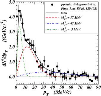
Figure 1: (Color Online) Comparison of normalized anomalous soft photon $dN^{\gamma}/dp_{T}$ per $pp$ collision at 450 GeV/c after subtracting the bremsstrahlung contributions Bel02 ; Per10 with calculated distributions based on three components of anomalous soft photons at 17, 45, and 5 MeV. The solid curve is the total theoretical $dN^{\gamma}/dp_{T}$ distribution, and the other curves are the separate contributions from the three different components.

According to the Schwinger’s mechanism Sch51 ; Won94a ; Wan88 ; Won95 , the probability of particle production is an exponential function of the square of the transverse mass of the produced particle. For massless photons, the photon transverse mass is the photon transverse momentum. It is therefore reasonable to assume the transverse momentum distribution of each photon component to be a Gaussian with an average root-mean-squared transverse momentum $M_{IT}^{\gamma}$ given by the QED2 photon mass. In the measurement of the soft photon transverse momentum distribution in $e^{+}$-$e^{-}$ annihilations, the determination of the orientation of jet axis has an uncertainty of $\Delta\theta$ $\sim$50 mrad, corresponding to a root-mean-square uncertainty of $\Delta p_{T}$ =$E_{\gamma}\Delta\theta$$\sim$10 MeV for the small $p_{T}$ region DEL06 . In the measurement of the transverse momentum distribution in $pp$ collisions, the uncertainty in angular measurements is $\Delta\theta$$\sim$10 mrad, which corresponds to $\Delta p_{T}$$\sim$2 MeV for the small $p_{T}$ region Bel02 . These uncertainties in the determination of the angles need to be folded into theoretical calculations in order to compare with experimental data. If one assumes a Gaussian distribution of the transverse coordinates in the angular determination, the folding of two Gaussian distributions leads to a Gaussian distribution with a standard deviation square of $[(M_{IT}^{\gamma})^{2}+(\Delta p_{T})^{2}]/2$.

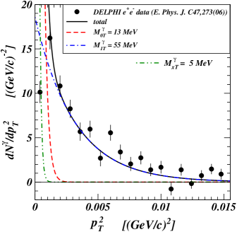
Figure 2: (Color Online) Solid points give the DELPHI experimental anomalous soft photon $dN^{\gamma}/dp_{T}^{2}$ data in $Z^{0}$ hadronic decay in $e^{+}$-$e^{-}$ annihilations, after subtracting the bremsstrahlung contributions DEL06 . The solid curve is the total theoretical $dN^{\gamma}/dp_{T}^{2}$ with contributions from component at 13 and 55 MeV, whose separate contributions are shown as the dashed and dashed-dot curves, respectively. The dashed-dot-dot curve gives the distribution for the lower momentum component at $M_{xT}^{\gamma}$=5 MeV, which however cannot be resolved in the present DELPHI measurements.

Based on our theoretical results in Table I, we expect that there will be two components in the soft photon transverse momentum spectrum. We therefore parametrize the experimental anomalous soft photon transverse momentum distribution as the sum of the two normalized Gaussian components of isoscalar and isovector photons, each of which has an average root-mean-squared transverse momentum given by $(M_{IT}^{\gamma})^{2}+(\Delta p_{T})^{2}$. We search for distributions characterized by a transverse mass in the region of $M_{0T}^{\gamma}$$\sim$25 MeV for the isoscalar photon and around $M_{1T}^{\gamma}$$\sim$44 MeV for the isovector photon component. However, upon a careful examination of the transverse momentum distribution of the anomalous soft photons in $pp$ collisions Bel02 , we find that in addition to these isoscalar and isovector photon components, the $pp$ data appears to contain an additional lower momentum component characterized by a small mass $M_{{x}T}^{\gamma}$. We need to parametrized it as arising from three contributions:

$$\frac{dN^{\gamma}}{dp_{T}^{2}}=\sum_{I=0,1}\frac{N_{I}^{\gamma}}{(M_{IT}^{\gamma})^{2}+(\Delta p_{t})^{2}}\exp\left\{-\frac{p_{T}^{2}}{(M_{IT}^{\gamma})^{2}+(\Delta p_{T})^{2}}\right\}+\frac{N_{x}^{\gamma}}{(M_{{x}T}^{\gamma})^{2}+(\Delta p_{t})^{2}}\exp\left\{-\frac{p_{T}^{2}}{(M_{{x}T}^{\gamma})^{2}+(\Delta p_{T})^{2}}\right\},$$ (53)

where the coefficients $N_{i}^{\gamma}$ are the integrated numbers of QED2 photons of mass $M_{iT}^{\gamma}$ produced per event.

The small transverse momentum uncertainties and the extension of the experimental data down to small values of $p_{T}$ in $pp$ collisions make it useful to examine first the transverse momentum distribution in $pp$ collisions. In Fig. 1 we show the experimental normalized $dN_{\gamma}/dp_{T}$ of anomalous soft photons per $pp$ collision event at 450 GeV/c from Fig. 2b of Ref. Bel02 ; Per10 , after subtracting the bremsstrahlung contributions. The $dN^{\gamma}/dp_{T}$ data for $pp$ collisions in Fig. 1 can be explained by assuming three anomalous soft photon contributions with parameters

$$M_{0T}^{\gamma}=17{\rm~{}MeV},M_{1T}^{\gamma}=45{\rm~{}MeV},M_{xT}^{\gamma}=5{\rm~{}MeV},N_{0}^{\gamma}=0.040,N_{1}^{\gamma}=0.017,{\rm~{}and~{}}N_{x}^{\gamma}=0.021.$$ (54)

We examine next the anomalous soft photon transverse momentum distribution in $e^{+}$-$e^{-}$ annihilations DEL06 . With an error of $\Delta p_{T}$ as large as 10 MeV, the distribution cannot be sensitive to the component at $M_{xT}\sim 5$ MeV. We show in Fig. 2 the DELPHI experimental $dN^{\gamma}/dp_{T}^{2}$ data from Fig. 4f of Ref. DEL06 , after subtracting the inner bremsstrahlung contributions. The experimental data can be explained by assuming the following set of parameters,

$$M_{0T}^{\gamma}=13{\rm~{}MeV},M_{1T}^{\gamma}=55{\rm~{}MeV},N_{0}^{\gamma}=0.106{\rm~{}and~{}}N_{1}^{\gamma}=0.058.$$ (55)

There are no reliable data points at $p_{T}^{2}<0.001$ (GeV/c)² to fix the $M_{xT}^{\gamma}$ component with the present $e^{+}$-$e^{-}$ data. For illustrative purposes, we show the $M_{xT}^{\gamma}$ component calculated with $M_{xT}^{\gamma}$=5 MeV and $N_{x}^{\gamma}/N_{0}^{\gamma}$=0.525 (as in Eq. (54)) shown as the dashed-dot-dot curve in Fig. 2, to indicate that its presence or absence has little effects on the theoretical results above $p_{T}>0.001$ GeV².

Our comparison of the anomalous soft photon transverse momentum distributions reveals that it is necessary to examine the transverse momentum distributions of both $pp$ collisions and $e^{+}$-$e^{-}$ annihilations as complimentary data sets, as the $pp$ data have finer resolution and smaller errors in the lower $p_{T}$$\sim$15 MeV regions while the $e^{+}$-$e^{-}$ data have less fluctuations in the higher $p_{T}$$\sim$50 MeV region. The combined analysis indicates that the transverse momentum spectrum can be qualitative described by two components with transverse masses of $\sim$15 MeV and $\sim$50 MeV, in approximate agreement with the gross features of the theoretical QED2 photon model. There is however an additional, lower momentum component at $\sim$5 MeV which shows up in $pp$ collisions, but cannot be resolved in $e^{+}$-$e^{-}$ annihilations. The origin of this low-$p_{T}$ component is not known and will be left for future studies. Among many possibilities, it may be the manifestation of the zero mode of QED2 photon production whose investigation will be of great future interest.

VII Rates of Meson and Anomalous Soft Photon Production

We shall now examine the remaining feature concerning the rates of meson and anomalous soft photon production in high-energy $e^{+}$-$e^{-}$ annihilations to complete our comparison of the QED2 model with experimental data. There are many important physical quantities in the production processes. The receding quark and antiquark generate a QCD field of strength $\kappa_{q\bar{q}}^{h}$ and a QED field of strength $\kappa_{q\bar{q}}^{\gamma}$ between the quark and the antiquark in the flux tube that will produce the QCD mesons and the QED2 photons, respectively. Here, we have used the superscript $\alpha$=$h$ for hadron quantities and $\alpha$=$\gamma$ for photon quantities. Each of the field quanta is produced in a final state possessing a transverse momentum, and thus the mass that enters into the consideration of quanta production should be the transverse mass $M_{IT}^{\alpha}=\sqrt{(M_{I({\rm 4D})}^{\alpha})^{2}+p_{T}^{2}}$, which can be identified as the boson mass $M_{I({\rm 2D})}^{\alpha}$ in two-dimensional space-time as discussed in Section V.

To obtain an estimate, we can rely on the Schwinger mechanism of particle production in a strong field as a guide Sch51 ; Won94a ; Wan88 ; Won95 . The probability of particle production of a composite particle of transverse mass $M_{IT}^{\alpha}$ depends on the exponential factor of $\exp\{-\pi(M_{IT}^{\alpha}/2)^{2}/\kappa_{q\bar{q}}^{\alpha}\}$, where the factor of 1/2 in $M_{IT}^{\alpha}/2$ is to denote the production of a pair of particles each of which has a mass $M_{IT}^{\alpha}/2$, and the binding of one particle of mass $M_{IT}^{\alpha}/2$ with the neighboring particle of mass $M_{IT}^{\alpha}/2$ leads subsequently to a composite stable boson of mass $M_{IT}^{\alpha}/2+M_{IT}^{\alpha}/2$. Furthermore, from dimensional analysis, we can infer that the rate of production per space-time volume element $(dz\,dt)$ has the dimension $\kappa_{q\bar{q}}^{\alpha}$. We therefore assume that the rate of the production of the number of particle of type $\alpha$, isospin $I$, and mass $M_{IT}^{\alpha}$ due to the presence of the QCD and QED fields between a receding quark $q$ and an antiquark $\bar{q}$ is

$$\frac{dN_{I}^{\alpha}}{dz\,dt}=A\sum_{q\bar{q}}P_{q\bar{q}}~{}\kappa_{q\bar{q}}^{\alpha}~{}\exp\left\{-\frac{\pi(M_{IT}^{\alpha}/2)^{2}}{\kappa_{q\bar{q}}^{\alpha}}\right\},~{}~{}~{}\alpha=\gamma,h,$$ (56)

where $P_{q\bar{q}}$ is the probability for the quark-antiquark source pair to be a $u\bar{u}$ or $d\bar{d}$ pair, and $A$ is a dimensionless constant. In an $e^{+}$-$e^{-}$ annihilation at high energies, there is an equal probability for the quark-antiquark pair to be a $u\bar{u}$ or $d\bar{d}$ pair, and so $P_{u\bar{u}}=P_{d\bar{d}}=1/2$.

For the production of QCD2 mesons, the color electric field strength between the leading quark and antiquark is independent of the quark flavor quantum number. It is given by

$$\kappa_{u\bar{u}}^{h}=\kappa_{d\bar{d}}^{h}={g_{\rm QCD2}^{2}}/{2}=b.$$ (57)

For the production of QED2 photons, the electric field strength between the leading quark $q$ and antiquark $\bar{q}$ is given in terms of the electric charges of the quark and the antiquark as

$$\kappa_{q\bar{q}}^{\gamma}=|Q_{q}Q_{\bar{q}}|e_{\rm QED2}^{2}/2.$$ (58)

Thus, we find that between a receding $q$ and $\bar{q}$, there is a constant electric field with a strength

$$\kappa_{u\bar{u}}^{\gamma}=0.002048{\rm~{}GeV}^{2},$$ (59a)

$$\kappa_{d\bar{d}}^{\gamma}=0.000512{\rm~{}GeV}^{2}.$$ (59b)

The QCD field strength $\kappa_{q\bar{q}}^{h}$ and the experimental meson transverse masses as given in Eqs. (51) and (52) allow us to determine from (56) the number of mesons (in a particular $I_{3}$ state) produced in a space-time volume of $\Delta z\Delta t$. Similarly, the QED field strength $\kappa_{q\bar{q}}^{\gamma}$, the QED2 photon isoscalar photon mass of $M_{0T}^{\gamma}$$\sim$15 MeV, and the isovector photon mass of $M_{1T}^{\gamma}$$\sim$50 MeV from Eqs. (54) and (55) allow us to determine the number of photons produced. We obtain,

$$N_{1}^{h} = A\Delta z\Delta t\times 0.05368{\rm~{}GeV}^{2},$$ (60a)

$$N_{0}^{h} = A\Delta z\Delta t\times 0.01391{\rm~{}GeV}^{2},$$ (60b)

$$N_{1}^{\gamma} = A\Delta z\Delta t\times 0.0003980{\rm~{}GeV}^{2},$$ (60c)

$$N_{0}^{\gamma} = A\Delta z\Delta t\times 0.0011206{\rm~{}GeV}^{2}.$$ (60d)

In these estimates, the number of produced particles of different types and isospin quantum numbers are proportional to the same space-time volume $\Delta z\Delta t$. This space-time volume fluctuates in each $Z^{0}$ hadronic decay event; the number of mesons and photons of different isospin quantum numbers will vary from event to event. However, because all these particles in each event are produced simultaneously by the fragmentation of the same $q$-$\bar{q}$ string and the same space-time volume, the ratio of different isospin spin quantum numbers and types of particles can therefore be proportional, on an event-by-event basis. The results in Eq. (60) give

$$\frac{N_{0}^{\gamma}}{N_{1}^{\gamma}}\sim\frac{11}{4},~{}~{}~{}\frac{N_{0}^{h}}{N_{1}^{h}}\sim\frac{1}{4},$$ (61)

which reveal that isoscalar photons are more preferentially produced than isovector photons whereas isoscalar mesons are much less likely produced than isovector meson (in a particular $I_{3}$ state). The theoretical ratio of $N_{0}^{\gamma}/N_{1}^{\gamma}$=2.8 compares approximately well with the experimental ratio of $N_{0}^{\gamma}/N_{1}^{\gamma}$$\sim$2.4 and 1.8 in Eq. (54) and (55) extracted by fitting the experimental transverse momentum distribution data of Bel02 and DEL06 . Using these results, we can also construct the ratio of ratios,

$$\frac{N_{0}^{\gamma}}{N_{0}^{h}}:\frac{N_{1}^{\gamma}}{N_{1}^{h}}\sim\frac{11}{4}:\frac{1}{4}=11:1,$$ (62)

which states that the number of soft isoscalar photons associated with the isoscalar meson production are more numerous than soft isovector photons associated with the isovector meson production.

The DELPHI experimental measurements DEL09 ; Per09 provide information on the ratios of anomalous soft photon production with various produced neutral or charged meson multiplicities. To compare with experimental data, we need to convert the number of different species of mesons to the number of charged and neutral mesons. Isovector mesons are pions which have two charged states and one neutral states, and each isoscalar $\eta$ meson decays into 1.64 neutral particles (with 2 $\gamma$’s counted as a $\pi^{0}$ as in Ref. DEL09 ) and 0.57 charged particles. Thus, the total meson particle number is $N_{\rm par}=(1.64+0.57)N_{0}^{h}+3N_{1}^{h}$. From Eq. (60), the theoretical ratio of total soft photons to total meson particles (charged and neutral) is

$$\frac{N^{\gamma}}{N_{\rm par}}\sim\frac{N_{0}^{\gamma}+N_{1}^{\gamma}}{2.21N_{0}^{h}+3N_{1}^{h}}=7.91\times 10^{-3},$$ (63)

which compares reasonably well with the experimental ratio of $N^{\gamma}/N_{\rm par}\sim 9.1\times 10^{-3}$.

In our QED2 photon model, production of mesons of isospin quantum number $I$ will be associated with the production of QED2 photons of the same isospin quantum number $I$. Thus, isoscalar QED2 photons will be associated with isoscalar mesons while isovector QED2 photons will be associated with isovector mesons.

From Eqs. (60d) and (60b), the theoretical ratio of the number of produced isoscalar photon to the number of produced isoscalar meson is

$$\frac{N_{0}^{\gamma}}{N_{0}^{h}}=80.6\times 10^{-3}.$$ (64)

As each isoscalar meson produces 1.641 neutral $\pi^{0}$-like particles and $0.57$ charged particles, the isoscalar meson is associated with the production of dominantly neutral mesons. As we consider the production of isoscalar mesons to be associated only with the production of isoscalar photons, then for the isoscalar mode of production, $N^{\gamma}/N_{\rm neu}\sim N_{0}^{\gamma}/N_{\rm neu}$ which leads to $N^{\gamma}/N_{\rm neu}\sim N_{0}^{\gamma}/(1.641N_{0}^{h})$ after summing over all charged particles. From Eq. (64), the theoretical ratio of soft photon to neutral particle number is

$$\frac{N^{\gamma}}{N_{\rm neu}}\sim\frac{N_{0}^{\gamma}}{1.641N_{0}^{h}}=49.1\times 10^{-3},$$ (65)

which comes close to the experimental ratio of $N^{\gamma}/N_{\rm neu}\sim 37.7\times 10^{-3}$.

Table 2: Comparison of QED2 photon model description of the anomalous soft photon production with quantities measured or extracted from the $pp$ collision Bel02 and DELPHI $e^{+}$-$e^{-}$ annihilation experimental data DEL06 ; DEL09 ; Per09

Quantities	QED2 Model	Experimental Anomalous Soft Photon Data
Isoscalar photon mass $M_{0}$	$O(25$ MeV)	$\sim$15 MeV
Isosvector photon mass $M_{1}$	$O(44$ MeV)	$\sim$50 MeV
$N_{0}^{\gamma}/N_{1}^{\gamma}$	11/4	1.8-2.4
$N^{\gamma}/N_{\rm par}$	7.91$\times 10^{-3}$	9.1$\times 10^{-3}$
$N^{\gamma}/N_{\rm neu}$	49.1$\times 10^{-3}$	37.7$\times 10^{-3}$
$N^{\gamma}/N_{\rm ch}$	3.71$\times 10^{-3}$	6.9$\times 10^{-3}$

From Eqs. (60c) and (60a), the theoretical ratio of the number of produced isovector photon to the number of produced isoscalar meson in a particular $I_{3}$ state is

$$\frac{N_{1}^{\gamma}}{N_{1}^{h}}=7.41\times 10^{-3}.$$ (66)

The isovector meson is three-fold degenerate with two charged particles and one neutral particle. Thus, the production of an isovector meson is associated with the production of dominantly charged particles. In the QED2 photon model, the sources of isospin current disturbances that produce the mesons and photons are the same. Therefore, the production of isovector mesons is associated only with the production of isovector photons. Consequently, we have $N^{\gamma}/N_{\rm ch}\sim N_{1}^{\gamma}/N_{\rm ch}$, which leads to $N^{\gamma}/N_{\rm ch}\sim N_{1}^{\gamma}/(2N_{1}^{h})$ after summing over all neutral particles. Equation (66) then leads to

$$\frac{N^{\gamma}}{N_{\rm ch}}\sim\frac{N_{1}^{\gamma}}{(2N_{1}^{h})}=3.71\times 10^{-3},$$ (67)

which is slightly less than the experimental ratio $N_{\gamma}/N_{\rm ch}\sim 6.9\times 10^{-3}$, but is within the same order of magnitude.

As a summary, we give the comparisons of various quantities obtained in the QED2 model with the DELPHI data DEL06 ; DEL09 ; Per09 in Table II. We conclude from the comparison that gross features of the DELPHI data is approximately consistent with the QED2 photon model.

VIII Further Experimental Tests of the QED2 Photon Model

While the QED2 photon model appears to explain qualitatively the main features of the experimental anomalous soft photon data, it is desirable to carry out further experimental measurements to test the model:

1. It will be of interest to measure the transverse momentum distribution of the soft photons with a finer $p_{T}$ resolution and greater precision for a given narrow range of photon rapidities. Qualitatively, we expect the production of photons with two different average transverse momenta, one at $\sim$15 MeV for the production of the isoscalar photon and one at $\sim$50 MeV for the production of the isovector photon.

2. It will be necessary to confirm the presence of the low momentum component at $M_{xT}^{\gamma}$=5 MeV in high-energy $e^{+}$-$e^{-}$ annihilation experiments. As the origin and the properties of such a low $p_{T}$ component is still unknown, additional experimental information on this source of anomalous soft photons will improve our understanding of such a component.

3. It will be of interest to measure the transverse momentum distribution by selecting events with predominantly neutral particles and events with predominantly charged particles. The former events will likely arise from the production of isoscalar mesons and QED2 isoscalar photons, with an average photon transverse momentum of $\sim$15 MeV, while the latter from the production of isovector mesons and the isovector photons, with an average photon transverse momentum of $\sim$50 MeV.

4. The rapidity distribution of the produced photons should exhibit the plateau structure, as expected of similar distributions in meson production. A measurement of the rapidity distribution will provide useful additional information on the dynamics of soft photon production.

5. Measurements of the properties of associated hadrons similar to those of the DELPHI Collaboration should be carried out with hadron-hadron collisions at high energies where anomalous soft photon production has been reported Chl84 ; Bot91 ; Ban93 ; Bel97 ; Bel02 ; Bel02a .

IX Conclusions and Discussions

A color flux tube is formed when a quark and an antiquark (or a diquark) pull apart from each other at high energies. The motion of the quarks in the underlying vacuum of the flux tube generates color charge oscillations which lead to the production of mesons. As a quark carries both a color charge and an electric charge, the color charge oscillations of the quarks in the vacuum are accompanied by electric charge oscillations, which will in turn lead to the simultaneous production of soft photons during the meson production process.

To study these density oscillations, we start with quarks interacting with both QCD and QED interactions in four-dimensional space-time in the U(3) group which breaks into the color SU(3) and the QED U(1) subgroups. Specializing to particle production at high energies, we find that the dominance of the longitudinal motion and transverse confinement lead to the compactification from QED4$\times$QED4 in four-dimensional space-time to QCD2$\times$QED2 in two-dimensional space-time, with the formation of the flux tube. In the flux tube, the self-consistent coupling of quarks and gauge fields lead to color charge and electric charge oscillations that give rise to stable QCD2 bosons and QED2 bosons. The boson masses depend on the gauge field coupling constants. The presence of the flavor degrees of freedom leads to isospin dependence of the boson masses, with the isovector meson mass smaller than the isoscalar meson mass, but the mass ordering is reversed for the isoscalar photon and the isovector photon.

As QCD2 and QED2 bosons are stable in the flux tube environment, we can infer from the quantum field theory description of particle production in Ref. Cas74 that these QCD2 mesons and QED2 photons will be produced simultaneously in $q$-$\bar{q}$ string fragmentation. Under the condition of adiabaticity with no change of the particle energy and longitudinal momentum after the produced particle emerges from the production region, the boson mass in two-dimensional space-time turns into the boson transverse mass in four-dimensional space-time.

The QED2 photon model can explain various features of the anomalous soft photon phenomenon. Because both color charge oscillations and electric charge oscillations arise from the same density oscillations of the quarks in the vacuum, both QCD2 meson and QED2 photon will be simultaneously produced by the fragmentation of the $q$-$\bar{q}$ string. These features are in agreement with those observed in DELPHI experiments DEL08 ; DEL09 ; Per09 . The transverse momentum distributions of anomalous soft photons in $pp$ collisions Bel02 and $e^{+}$-$e^{-}$ annihilations DEL06 can be described by a component with $M_{0T}^{\gamma}$$\sim$15 MeV and a component at $M_{1T}^{\gamma}$$\sim$50 MeV in approximate agreement with theoretical estimates of the order of the isoscalar and isovector QED2 photon masses.

In the QED2 model, there are important and non-trivial isospin dependencies in the rate of photon and hadron productions that is consistent with recent DELPHI data. The model predicts that the isoscalar photon mass is lower than the isovector photon mass. Consequently, the production of isoscalar photons is more likely than isovector photons. In contrast, the QCD isoscalar meson mass is greater than the isovector mass, the production of isoscalar mesons is less likely than isovector mesons. Thus, the ratio of $N_{0}^{\gamma}/N_{0}^{h}$ can be much greater than $N_{1}^{\gamma}/N_{1}^{h}$. The production of isoscalar hadrons is associated with the production of isoscalar photons and leads predominately to neutral particles while the production of isovector hadrons is associated with the production of isovector photons and leads predominantly to charged particles. As a consequence, the ratio $N^{\gamma}/N_{\rm neu}$ is much greater than the ratio $N^{\gamma}/N_{\rm ch}$, as observed by the DELPHI Collaboration DEL09 ; Per09 .

Although the QED2 photon model appears to be promising, it is desirable to carry out additional experimental measurements to test the model. We suggest the search for the two components of transverse momentum distributions by making appropriate cuts in soft photon rapidities and selecting different regions of neutral and charge multiplicities where different isospin photon components are expected. The identification of the two components of different soft photon transverse momenta will be a crucial test of the QED2 photon model in the QCD string fragmentation process.

Our examination of the transverse momentum distribution of anomalous soft photons in $pp$ collisions in Bel02 reveal the presence of an additional component characterized by a transverse mass of $M_{xT}^{\gamma}$=5 MeV. What is the nature of this component? Is it related to the zero mode of density oscillations? How does the zero mode manifest itself experimentally? Experimental investigation of the low transverse momentum component of photon production and the theoretical investigation of the zero mode of QED2 photon production will be of great future interest.

There are puzzling elements of the QED2 photon model that call for future theoretical and experimental resolution. As it now stands, the theoretical determination of the QED2 photon masses is rather uncertain as the mass scale $\mu$ in the bosonization of the scalar density is unknown. The QED2 photon mass scale as extracted from experimental data requires an electromagnetic current quark mass smaller than the current quark mass as determined from perturbative QCD. Whether or not such a smaller value of the mass scale $\mu$ for the anomalous soft photon production is justified will require further theoretical and experimental investigations.

Another puzzling and unresolved question is the more detail description of the evolution from a QED2 photon to a QED4 photon. We have used the concept of adiabaticity so that the photon preserves its energy and longitudinal momentum, only to develop a transverse momentum to balance the mass shell condition. Such a description appears to give a qualitative description of the transverse momenta and production probabilities of the soft photons. However, there is no additional content in the dynamics of the evolution in our hypothesis. A more detail dynamics of the evolution of QED2 to QED4 will be of great interest.

Finally, if the model is proved to be successful in explaining the anomalous soft photon data, it may be useful to explore whether one can study this non-perturbative problem in the full four-dimensional space-time without resorting to the intermediate stage of going through the two-dimensional space-time, where non-perturbative physics can be carried out more readily. The success of a completely four-dimensional description will provide new insight into the non-perturbative behavior of particle production in strong fields.

Acknowledgment

The author would like to thank Dr. V. Perepelitsa for stimulating discussions and valuable information on DELPHI anomalous soft photon experimental data. The author also wishes to thank Drs. H. Crater and T. Barnes for helpful discussions. The research was sponsored by the Office of Nuclear Physics, U.S. Department of Energy.

References

- (1) P.V. Chliapnikov et al., Phys. Lett. B 141, 276 (1984).
- (2) F. Botterweck et al., Z. Phys. C 51, 541 (1991).
- (3) S. Banerjee et al., Phys. Lett. B 305, 182 (1993).
- (4) A. Belogianni et al.,Phys. Lett. B 408, 487 (1997).
- (5) A. Belogianni et al.,Phys. Lett. B 548, 129 (2002).
- (6) A. Belogianni et al.,Phys. Lett. B 548, 122 (2002).
- (7) J. Abdallah (DELPHI Collaboration), Eur. Phys. J. C 47, 273 (2006).
- (8) DELPHI Collaboration, J. Abdallah et al., CERN Report PH–EP 2009-014, [arXiv:1004.1587], accepted for publication in European Physical Journal C.
- (9) V. Perepelitsa, for the DELPHI Collaboration, Proceedings of the XXXIX International Symposium on Multiparticle Dynamics, Gomel, Belarus, September 4-9, 2009.
- (10) J. Abdallah (DELPHI Collaboration), Eur. Phys. J. C 57, 499 (2008).
- (11) V. Balek, N. Pisutova, and J. Pisut, Acta. Phys. Pol. B21, 149 (1990).
- (12) P. Lichard, Phys. Rev. D50, 6824 (1994).
- (13) L. Van Hove, Ann. Phys. (N.Y.) 192, 66 (1989); P. Lichard and L. Van Hove, Phys. Lett. B 245, 605 (1990).
- (14) W. Czyz and W. Florkowski, Z. Phys. C61, 171 (1994).
- (15) E. Kokoulina, A. Kutov, V. Nikitin, Braz. J. Phys., 37, 785 (2007); M. Volkov, E. Kokoulina, E. Kuraev, Ukr. J. Phys., 49, 1252 (2003).
- (16) S.M. Darbinian, K.A. Ispirian, A.T. Margarian, Sov. J. Nucl. Phys. 54, 364 (1991).
- (17) O. Nachtmann, hep-ph/9411345; G.W. Botz, P. Haberl, O. Nachtmann, Z. Phys. C 67, 143 (1995).
- (18) B. Andersson, G. Gustafson, and T. Sjöstrand, Zeit. für Phys. C20, 317 (1983); B. Andersson, G. Gustafson, G. Ingelman, and T. Sjöstrand, Phys. Rep. 97, 31 (1983); T. Sjöstrand and M. Bengtsson, Computer Physics Comm. 43, 367 (1987); B. Andersson, G. Gustavson, and B. Nilsson-Alqvist, Nucl. Phys. B281, 289 (1987).
- (19) Yu.A. Simonov, Phys. Atom. Nucl., 71, 1049 (2008), hep-ph/07113626; Yu.A. Simonov, JETP Lett., 87, 147 (2008) Yu.A. Simonov, A.I. Veselov, JETP Lett., 88, 79 (2008); Yu.A. Simonov, A.I. Veselov, Phys. Lett. B 671, 55 (2009).
- (20) Yoshitaka Hatta and Takahiro Ueda, arXiv:arXiv:1002.3452.
- (21) A. Casher, J. Kogut, and L. Susskind, Phys. Rev. D10, 732 (1974).
- (22) S. Coleman, Ann. Phys. 101, 239 (1976).
- (23) J. Schwinger, Phys. Rev. 128, 2425 (1962); J. Schwinger, in , Trieste Lectures, 1962 (I.A.E.A., Vienna, 1963), p. 89.
- (24) J. H. Lowenstein and J. A. Swieca, Ann. Phys. (N.Y.) 68, 172 (1971).
- (25) S. Coleman, R. Jackiw, and L. Susskind, Ann. Phys. 93, 267 (1975).
- (26) J. D. Bjorken, Lectures presented in the 1973 Proceedings of the Summer Institute on Particle Physics, edited by Zipt, SLAC-167 (1973).
- (27) J. D. Bjorken, Phys. Rev. D 27, 140 (1983).
- (28) C. Y. Wong, R. C. Wang, and C. C. Shih, Phys. Rev. D 44, 257 (1991).
- (29) For a pedagogical discussion of QED2, see Chapter 6 of C. Y. Wong, Introduction to High-Energy Heavy-Ion Collisions, World Scientific Publisher, 1994.
- (30) C. Y. Wong, Phys. Rev. C80, 034908 (2009).
- (31) C. Y. Wong, Phys. Rev. C80, 054917 (2009).
- (32) G. Gatoff and C. Y. Wong, Phys. Rev. D46, 997 (1992); and C. Y. Wong and G. Gatoff, Phys. Rep. 242, 489 (1994).
- (33) H. Aihara (TPC/Two_Gamma Collaboration), Lawrence Berkeley Laboratory Report LBL-23737 (1988).
- (34) W. Hofmann, Ann. Rev. Nucl. Sci. 38, 279 (1988).
- (35) A. Petersen , (Mark II Collaboration), Phys. Rev. D 37, 1 (1988).
- (36) K. Abe (SLD Collaboration), Phys. Rev. D 59, 052001 (1999).
- (37) K. Abreu (DELPHI Collaboration), Phys. Lett. B 459, 397 (1999).
- (38) Hongyan Yang (BRAHMS Collaboration), J. Phys. G35, 104129 (2008); K. Hagel (BRAHMS Collaboration), APS DNP 2008, Oakland, California, USA Oct 23-27, 2008.
- (39) S. Mandelstam, Phys. Rev. D11, 3026 (1975).
- (40) M. B. Halpern, Phys. Rev. D12, 1684 (1975).
- (41) E. Witten, Commun. Math. Phy. 92, 455 (1984)
- (42) D. Gepner, Nucl. Phys. B 252, 481 (1985). J. Phys. A 31, 9925 (1998).
- (43) E. Abdalla, M. C. B. Abdalla, and K. D. Rothe, Two Dimensional Quantum Field Theory, World Scientific Publishing Company, Singapore, 2001.
- (44) Y. Frishman and J. Sonnenschein, Phys. Rep. 223, 309 (1993).
- (45) Y. Frishmann, A. Hanany, and J. Sonnenschein, Nucl. Phy. B429, 75 (1994).
- (46) A. Armonic and J. Sonnenschein, Nucl. Phy. B457, 81 (1995).
- (47) D. Gross, I. R. Klebanov, A. Matysin, and A. V. Smilga Nucl. Phys. B461, 109 (1996).
- (48) E. Abdalla and M.C.B. Abdalla, Phys. Reports 265, 253 (1996).
- (49) J. P. Vary, T. J. Fields, and H. J. Pirner, Phys. Rev. D53, 7231 (1996).
- (50) C. Adam, Ann. Phys. (N.Y.) 259, 1 (1997)
- (51) Y. Hosotani and R. Ridgriguez, J. Phys. A 31, 9925 (1998).
- (52) A. Armonic, Y. Frishmann, J. Sonnenschein, and U. Trittmann Nucl. Phy. B537, 503 (1999).
- (53) U. Trittmann, Phys. Rev. D66, 025001 (2002).
- (54) A. Abrashikin, Y. Frishmann, and J. Sonnenschein, Nucl. Phy. B703, 320 (2004).
- (55) A. Abrashikin, Y. Frishmann, and J. Sonnenschein, Talk presented by Y. Frishman at the Light-Cone Workshop in Cairns, Australia, July 2005, published in Nucl. Phys. Proc. Suppl. 161, 2, 2006, hep-th/0510167.
- (56) M. Engelhardt, Phys. Rev. D64, 065004 (2001).
- (57) C. Adam, Phys. Lett. B555, 132 (2003).
- (58) S. Nagy, Phys. Rev. D79, 045004 (2009).
- (59) Compared to the result of Ref. Col76 , Eq. (36) contains an extra factor of 1/2 which arises in the scale we have chosen to define with Eq. (27), where tr= for non-Abelian bosonization. If we choose a differently scaled boson field with , then there will be no extra factor of 1/2 in the Hamiltonian density with the fields.
- (60) The mass of the massive boson in multiflavor QCD2 was given as = in Arm99 ; Abr04 but as = in Tri02 ; Abr05 . In our comparison, we shall quote only the latest result, = of Ref. Abr05 , which comes from the same group of authors and presumably has included the latest typographical and other corrections.
- (61) R. Barate (ALEPH Collaboration), Zeit. Phys. C 74, 451 (1997).
- (62) C. Amsler (Particle Data Group), Phys. Lett B667, 1 (2008).
- (63) J. Schwinger, Phys. Rev. 82, 664 (1951).
- (64) R. C. Wang and C. Y. Wong, Phys. Rev. D38, 348 (1988).
- (65) For a pedagogical discussion of Schwinger particle production mechanism, see Chapter 5 of C. Y. Wong, Introduction to High-Energy Heavy-Ion Collisions, World Scientific Publisher, 1994.
- (66) C. Y. Wong, R. C. Wang, and J. S. Wu, Phys. Rev. D51, 3940 (1995).
- (67) We have converted the distribution of Fig. 2b of Ref. Bel02 , given in unnormalized numbers of counted photons per (2 MeV/c), to the normalized of Fig. 1, in numbers of photons per GeV/c per event, following a private communication from Dr. V. Perepelitsa by noting that the numbers of photons counted in Ref. Bel02 correspond to 4,000,000 events.