Square Lattice Gases with Two- and Three-body
Interactions Revisited

Abstract

Monte Carlo simulations have been used to study the phase diagrams for square Ising-lattice gas models with two-body and three-body interactions for values of interaction parameters in a range that has not been previously considered. We find unexpected qualitative differences as compared with predictions made on general grounds.

I Introduction

Experimental studies of phase transitions in adsorbed monolayers have resulted in examination of order-disorder transitions in lattice gas Ising models which represent the occupation of the periodic minima in the substrate potentialdas78 ; bin89 . Such models, usually containing two or more competing two-body interactions, have been studied by Monte Carlo simulationsbin80 ; bin82 which have determined the location and nature of the resultant phase boundaries. Typical ordered phases which are found for square lattice models with near-neighbor coupling are shown in Fig. 1 along with low density and high density disordered states termed lattice gas (L.G.) and lattice liquid (L.L.), respectively.

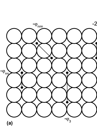
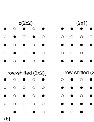
Figure 1: (a) Schematic view of the (100) surface of a substrate whose periodic potential provides a square lattice of preferred adsorption sites. The interactions used in this study are shown schematically as straight lines between adatoms which are represented by the filled circles. (b) Unit cells of the ordered overlayer structures discussed in the text.

Experimentally observed asymmetries in phase boundaries as a function of coverage can be explained by lattice gas models if three-body interactions are introduced as well. Theoretical studies of adatom-adatom interactions find surface mediated many-body couplingsein73 . A square lattice model with first- and second-neighbor two-body coupling and weak three-body interactions was investigatedbin81 in an attempt to clarify the phase transitions for H on Pd(001) and predictions were made for the case of even larger three-body coupling. Monte Carlo simulations showed that the inclusion of three-body interactions did make the transition asymmetric about 50 percent coverage and could even force the tricritical point on one side of the phase boundary to zero temperature. Such an asymmetry can also be interpreted in another form of non-additive interactionsmil81 , and a recent Monte Carlo study shows the effect of various cases of strength of interactionspin08 .

In this paper, we present the results of an investigation of the model proposed in Ref bin81 with moderate to large three-body interactions using Monte Carlo simulations. In the next section, we shall review some appropriate background and in Sec. III we present our results for two different values of interaction parameters which yield qualitatively different phase diagrams. We conclude in Sec. IV.

II Background

A lattice gas model is a collection of atoms whose positions may take on only discrete positions which form a periodic array, in this case a simple square lattice. A configuration of this lattice is defined by site occupation variables $c_{i}$ where $c_{i}=1$ if site $i$ is occupied and $c_{i}=0$ if the site is empty. The Hamiltonian which we use includes interaction $\varphi_{nn}$ between nearest-neighbors, $\varphi_{nnn}$ between next-nearest-neighbors, and $\varphi_{t}$ between neighbors on a triangle inscribed within a square made up of nearest-neighbors:

$${\cal H}-\mu N_{a}= - (\epsilon+\mu)\sum_{i}c_{i}-\varphi_{nn}\sum_{i\neq j}c_{i}c_{j}$$ (1)

$$- \varphi_{nnn}\sum_{i\neq k}c_{i}c_{k}-\varphi_{t}\sum_{i\neq j\neq k}c_{i}c_{j}c_{k},$$

and the coverage of the lattice is given by

$$\theta=\sum_{i}c_{i}$$ (2)

This model may be transcribed to the Ising model by the transformation to spin variables $\sigma=1-2c_{i}$, thus giving rise to the Hamiltonian

$${\cal H}= - H\sum_{i}\sigma_{i}-J_{nn}\sum_{i\neq j}\sigma_{i}\sigma_{j}$$ (3)

$$- J_{nnn}\sum_{i\neq k}\sigma_{i}\sigma_{k}-J_{t}\sum_{i\neq j\neq k}\sigma_{i}\sigma_{j}\sigma_{k},$$

where the Ising model interaction parameters are related to the lattice gas couplings by

$$J_{nn}=\frac{1}{4}\varphi_{nn}+\frac{1}{2}\varphi_{t}$$ (4)

$$J_{nnn}=\frac{1}{4}\varphi_{nnn}+\frac{1}{4}\varphi_{t}$$ (5)

$$J_{t}=-\frac{1}{8}\varphi_{t}$$ (6)

$$H={-\frac{1}{2}}(\epsilon+\mu)-\varphi_{nn}-\varphi_{nnn}-\frac{3}{2}\varphi_{t}$$ (7)

The magnetization is then related trivially to the coverage

$$m=1-2\theta.$$ (8)

Because of technical considerations, it is generally easier to carry out simulations in the magnetic (Ising) representation, and additional symmetries often become obvious in this approach. For example, in the Ising representation it is easy to see that the phase diagram must be symmetric in the absence of three-body interactions. Throughout the remainder of this paper we shall normalize all quantities by the nearest-neighbor coupling $J_{nn}$ and define $R=J_{nnn}/J_{nn}$ and $R_{t}=J_{t}/J_{nn}$. As a function of the relative strength of the three-body interactions, Binder and Landau suggested four different schematic phase diagrams (shown in Fig. 2) to describe the range of possible behavior due to the inclusion of three-body coupling, and using Monte Carlo simulations verified the nature of the phase diagrams with weak three-spin coupling shown in the upper portion of Fig. 2.

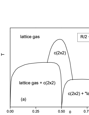
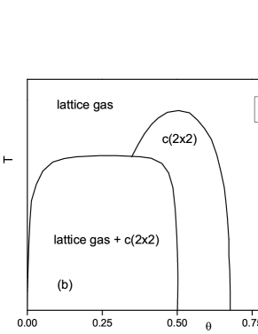
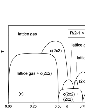
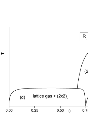
Figure 2: Possible schematic temperature-coverage phase diagrams for various choices of $R_{t}$ (from Ref.  bin81 ).

The remaining two diagrams were not based on any explicit calculation but were guessed as extensions of what was then believed to be the field-dependent behavior in the absence of three-spin interactions. Our views of the correct behavior in this latter case have changed, and given the complexity of phase diagrams in other two-dimensional systems with competing interactions, the predictions should be regarded with care.

At $T=0$ the energies of each ordered state as well as the lattice gas and lattice liquid phases may be calculated without difficulty and the intersections of the energy vs. chemical potential lines locate the transitions between neighboring phases. Of course, this is also valid in the Ising representation, and in Fig. 3 we show the ground state phase diagrams as a function of $R_{t}$ and $H$ which we obtain for two different values of $R$ which are in the parameter region discussed by Binder and Landaubin81 but not actually simulated.

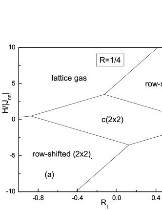
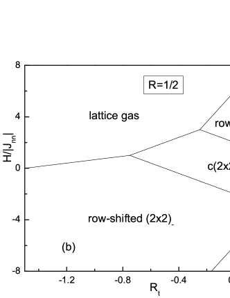
Figure 3: Groundstate phase diagrams for the Ising square lattice with pairwise and three-spin interactions: (a) $R=1/4$; (b) $R=1/2$.

One interesting feature of this diagram is that the $(2\times 2)$ state is actually degenerate in that either alternate rows or alternate columns may be shifted randomly by one lattice constant without any cost in energybin80 ; yin09 . This “row-shifted $(2\times 2)$” state has been seen before and the nature of the finite temperature transition to the disordered state is a matter of some disagreement. We believe that as long as the ground states do not change, the specific choice of parameters is not important and we have simply chosen values for which the $c(2\times 2)$ and row-shifted $(2\times 2)$ phases are stable over relatively large ranges of fields in Fig. 3 at which multiple phases become degenerate.

We have used the parallel tempering algorithm with GPU accelerated techniquesyin09 to study the thermodynamic properties of this model from which phase diagrams can be deduced. Spins were placed on $L\times L$ square lattices with periodic boundary conditions and were flipped using a Metropolis transition probability. Typically, $10^{6}$ to $10^{7}$ Monte Carlo steps are used to collect data for each run and 3 to 6 independent runs are taken to calculate standard statistical error bars, and in all the plots of data and analysis shown in following sections, if error bars are not shown they are always smaller than the size of the symbols. Lattice sizes from $L=32$ to $L=300$ were simulated and the data were interpreted within the context of finite size scalingpri90 . Most of the simulations were carried out on a GeForce GTX285 graphics unit. In addition to internal energy, specific heat, and magnetization, we calculated order parameters, e.g., $m_{c(2\times 2)},m_{2\times 1}$, etc., for the various ordered states shown in Fig. 1, and 4th order cumulant $U$ is defined in terms of the order parameter accordingly.

III Results

A.    $R=1/4,R_{t}=-1/4$

Bulk properties such as the specific heat peak, temperature dependence of the 4th order cumulant of the order parameter, etc., were used to determine the location of phase transitions.

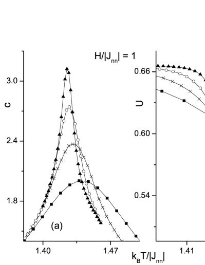
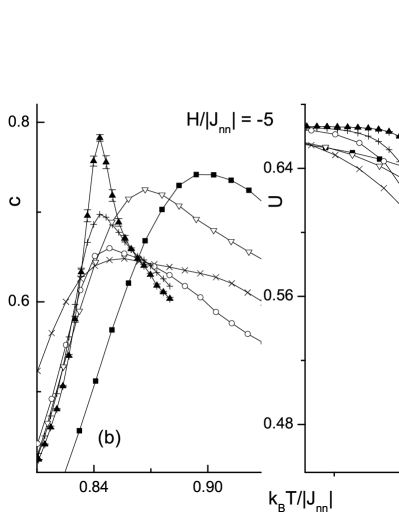
Figure 4: Bulk properties for $R=1/4,R_{t}=-1/4$: Specific heat $c$ and 4th order cumulant $U$ of the corresponding order parameter for (a) $H/|J_{nn}|=1$. Data are for: L=32, $\blacksquare$; L=64, $\times$; L=128, $\circ$; L=256, $\blacktriangle$. (b) $H/|J_{nn}|=-5$. Data are for L=30, $\blacksquare$; L=40, $\triangledown$; L=64, $\times$; L=128, $\circ$; L=168, $+$; L=256, $\blacktriangle$.

Sample data for the 4th order cumulant and specific heat are shown in Fig. 4; the specific heat peaks diverge with increasing lattice sizes for fields above $H/|J_{nn}|=-2.0$, but for fields more negative and close to the $c(2\times 2)$ phase boundary, the specific heat peaks first decrease and then diverge again with larger lattice sizes. Similar behavior was observed for the 4th order cumulant: for the small lattice, there is more than one diverging correlation length; but if the lattice sizes are big enough, only one dominates. Therefore, in certain range of small lattice sizes, the behavior is easy to confuse with XY-likekos73 , and GPU accelerated simulations of large lattice sizes is essential. For positive fields and low temperatures there is hysteresis in the m vs. H data indicating the presence of first-order transitions, but at higher temperature the data obtained for increasing and decreasing fields are essentially identical.

The resultant phase diagram in field-termperature space is shown in Fig. 5.

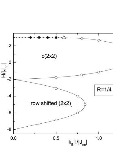
Figure 5: Phase diagram in magnetic field-temperature space for $R=1/4,R_{t}=-1/4$. The solid curves are second-order phase boundaries and the dashed line indicates first-order transitions. The open triangle indicates the location of a tricritical point.

The $c(2\times 2)$ phase is separated from the disordered phase on the high field side by a phase boundary which contains a tricritical point but on the low field side the transition appears to stay second-order down to the lowest temperature studied, and the row-shifted $(2\times 2)$ state is also bounded by a line of second order transitions. Since the transition from the $c(2\times 2)$ ordered phase to the disordered phase should belong to the Ising universality, we expect $\alpha/\nu=0$(logarithm) for a second-order phase transition, and $\alpha/\nu=2$ for a first-order phase transition. At the tricritical point, the exact(conjectured) value for the exponent $\alpha/\nu$ is $\frac{8}{5}$, which is supported by many renormalization group calculationsnij79 . Therefore, we estimate the exponent from finite size behavior of specific heat peaks, $c_{max}\sim L^{\alpha/\nu}$, near the connecting section of the first- and second-order transition line, and found the tricritical point is close to $k_{B}T/|J_{nn}|=0.592$. To confirm our estimation and get more accurate location, we also calculate the density distribution of the order parameter, as shown in Fig. 6. The final estimation of the tricirtial point is $k_{B}T/|J_{nn}|=0.5915(4),H/|J_{nn}|=2.98073(8)$, and the evaluated exponent $\alpha/\nu=1.59(2)$ agrees nicely with the predicted value.

Figure 6: Tricritical point(T=0.5915(4), H=2.98073(8)) for $R=1/4,R_{t}=-1/4$: (a) Curve fit of the specific heat peaks. (b) The density distribution of order parameter $M_{c(2\times 2)}$ for $L=256$.

The corresponding phase diagram in coverage-temperature space is shown in Fig. 7.

Figure 7: Temperature-coverage phase diagram for $R=1/4,R_{t}=-1/4$.

Here we see that the $c(2\times 2)$ phase and the L.G.+$c(2\times 2)$ coexistence phase, which is present below the tricritical point, appear over substantial ranges of $\theta$ and $T$, whereas the row-shifted $(2\times 2)$ phase is actually confined to a very narrow range of coverage. This phase diagram is substantially different from that predicted in Fig. 2c, and in particular there is no triple point. However, If third-nearest- neighbor two-body interactions are added, the ground state degeneracy for the $(2\times 2)$ state will be removed. Then, tricritical points involving the $(2\times 2)$ phase could occur, and triple points in the region of the first order transition perhaps as well, i.e., the predicted phase diagram in Fig. 2c could then be valid.

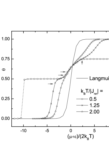
Figure 8: Adsorption isotherms of the lattice gas model with $R=1/4,R_{t}=-1/4$. The arrows mark the second-order phase transitions.

In Fig. 8 we show adsorption isotherms which are obtained for several different temperatures and for comparison include the Langmuir isotherm which would be correct for a non-interacting lattice gas. The jump in the low temperature data shown by the dotted line clearly locates the first-order transition; but the second-order transitions, indicated by the arrows, are extremely difficult to identify from the adsorption isotherms. The step-like behavior of the lowest temperature adsorption isotherm shown in this figure is not dissimilar to the multiple risers which are seen for multilayer adsorption, but here it merely represents multiple transitions within a single layer!

B.    $R=1/2,R_{t}=-1$

The same thermodynamic properties were determined as were described in Sec. A, and since there were no significant differences in the nature of the results, we shall not show any raw data for this case. The resultant phase diagram in H-T space is shown in Fig. 9.

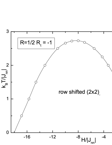
Figure 9: Field-temperature phase diagram for $R=1/2,R_{t}=-1$. The solid curves are second-order transitions and the dashed lines show first-order phase boundaries. The open square indicates the location of the terminating critical point.

A line of first-order transitions, terminating in a critical point, separates a lattice liquid from a lattice gas state, and a line of second-order transitions bounds a row-shifted $(2\times 2)$ phase.

Since the lack of symmetry among the two different phases at the critical point that terminates the first order line, the relevant scaling fields $\tau,h$ are comprised by linear combinations of the thermodynamic fields $T,H$ asreh73

$$\tau=T-T_{c}+s(H-H_{c})$$ (9)

$$h=H-H_{c}+r(T-T_{c})$$ (10)

where s and r are parameters controlling the extent of field mixing. As a result, the associated conjugate scaling operators ${\cal E},{\cal M}$ are also linear combinations of the spin-spin interaction energy density u and the magnetization m as

$${\cal E}=\frac{u-rm}{1-rs}\qquad\qquad\qquad\qquad$$ (11)

$${\cal M}=\frac{m-su}{1-rs}\qquad\qquad\qquad\qquad$$ (12)

$$m=\frac{1}{N}\sum_{i}\sigma_{i}\qquad\qquad\qquad\quad\enspace$$ (13)

$$u=\frac{1}{N}(\sum_{i\neq j}\sigma_{i}\sigma_{j}+R\sum_{i\neq k}\sigma_{i}\sigma_{k}+R_{t}\sum_{i\neq j\neq k}\sigma_{i}\sigma_{j}\sigma_{k})$$ (14)

where N is the total number of spins. According to the finite-size scalingbru92 , the joint probability distribution $p_{L}({\cal E},{\cal M})$ near criticality should obey the following scaling ansatz:

$$p_{L}({\cal E},{\cal M})\simeq\Lambda^{+}_{\cal M}\Lambda^{+}_{\cal E}\tilde{p}_{{\cal E},{\cal M}}(\Lambda^{+}_{\cal M}\delta{\cal M},\Lambda^{+}_{\cal E}\delta{\cal E},\Lambda_{\cal M}h,\Lambda_{\cal E}\tau)$$ (15)

where,

$$\Lambda_{\cal E}=a_{\cal E}L^{1/\nu},\quad\Lambda_{\cal M}=a_{\cal M}L^{d-\beta/\nu}$$ (16)

$$\Lambda_{\cal E}\Lambda^{+}_{\cal E}=\Lambda_{\cal M}\Lambda^{+}_{\cal M}=L^{d}\qquad\qquad$$ (17)

$$\delta{\cal M}={\cal M}-<{\cal M}>_{c},\quad\delta{\cal E}={\cal E}-<{\cal E}>_{c}$$ (18)

The subscripts c denotes that the averages are taken at criticality. For appropriate choices of the nonuniversal factors $a_{\cal E}$ and $a_{\cal M}$, function $\tilde{p}_{{\cal E},{\cal M}}$ would be universal. After integration over ${\cal E}$, exactly at criticality, where $h=\tau=0$, one has

$$p_{L}({\cal M})\simeq a_{\cal M}^{-1}L^{\beta/\nu}\tilde{p}^{*}_{\cal M}(L^{\beta/\nu}a_{\cal M}^{-1}\delta{\cal M})$$ (19)

where the function $\tilde{p}^{*}_{\cal M}$ characterizes the universality class, the form of which has been well established for the two-dimensional Ising model.

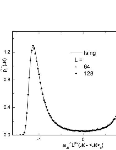
Figure 10: The density distributions for $L=64$ and $128$ at the critical point $k_{B}T/|J_{nn}|=2.2738(4),H/|J_{nn}|=1.24925(13)$. The full curve is the corresponding distribution for the two-dimensional Ising model for $L=400$.

In Fig. 10, we plot the density distribution function at estimated criticality $k_{B}T/|J_{nn}|=2.2738(4),H/|J_{nn}|=1.24925(13)$ with the controlling parameter $s=-0.30(2)$ for $L=64$ and $128$. The superimposed curve is the corresponding distribution for the two-dimensional Ising model for $L=400$. The nonuniversal factors $a_{\cal M}$ for each lattice sizes is chosen in such a way that the variable $a_{\cal M}^{-1}L^{\beta/\nu}({\cal M}-<{\cal M}>_{c})$ has unit variance.

As for the critical exponents for the continuous transition from the row-shifted $(2\times 2)$ phase to the paramagnetic phase, the correlation length exponent $\nu$ changes along the transition line, but the reduced exponents $\gamma/\nu$ and $\beta/\nu$ seems to belong to Ising universality, similar to what we found in Ref yin09 .

The phase diagram is replotted in coverage-temperature space in Fig. 11.

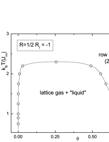
Figure 11: Temperature-coverage phase diagram for $R=1/2,R_{t}=-1$.

Here, too, we see that the row-shifted $(2\times 2)$ phase is present only over a relatively narrow range of coverages, but the L.G. + L.L. coexistence phase is stable over a much larger region of $T-\theta$ space. Comparing with Fig. 2d, we see that there are qualitative differences between the actual behavior and the phase diagrams which had previously been “guessed”; but again, if the degeneracy allowing for row-shifted structures were removed, the predicted phase diagram in Fig. 2d might hold.

IV Conclusions

Monte Carlo simulations have been used to extract phase diagrams for simple models on a square lattice with three-body interactions which are larger in magnitude than those which have been previously studied. We find qualitatively different behavior than that which had been suggested in Ref  bin81 . If third-nearest- neighbor two-body interactions are added, the ground state degeneracy for the $(2\times 2)$ state will be removed; but of course there is no guarantee that the finite temperature behavior will not show remnants of this effect. These results further demonstrate the complexity which may be found in relatively simple models with competing interactions. This problem is of interest to statistical mechanics in its own right and we believe that further Monte Carlo studies of such models will continue to display many of the features observed in experimental studies of adsorbed monolayers.

V Acknowledgements

We wish to thank T. L. Einstein and K. Binder for illuminating comments and suggestions, J. L. Li and C. W. Chen for sharing preliminary data, and S.-H. Tsai for providing the critical density distribution of the 2D Ising model for $L=400$. This research was supported in part by National Science Foundation grant DMR-0810223.

References

- (1) For reviews see J. G. Dash, Phys. Rep. 38C 177 (1978); E. Bauer, Structure and Dynamics of Surfaces II, edited by W. Schommers and P. von Blanckenhagen (Springer, Berlin, 1987); See also, Adv. Chem. Phys. Molecule Surface interactions, edited by K. P. Lawley (Wiley, London, 1989).
- (2) K. Binder and D. P. Landau, Adv. Chem. Phys., Molecule Surface Interactions, edited by K. P. Lawley, 91 (Wiley, London, 1989).
- (3) K. Binder and D. P. Landau, Phys. Rev. B 21 1941 (1980).
- (4) K. Binder, W. Kinzel, and D. P. Landau, Surf. Sci. 117 232 (1982); D. P. Landau, Phys. Rev. B 27 5604 (1983).
- (5) T. L. Einstein and J. R. Schrieffer, Phys. Rev. B 7 3679 (1973).
- (6) K. Binder and D. P. Landau, Surf. Sci. 108 503 (1981).
- (7) A. Milchev, M. Paunov, Surf. Sci. 108 25 (1981); A. Milchev, Electrochem. Acta 28 941 (1983).
- (8) O. A. Pinto, A. J. Ramirez-Pastor and F. Nieto, Surf. Sci. 602 1763 (2008).
- (9) Junqi Yin and D. P. Landau, Phys. Rev. E 80 051117 (2009).
- (10) See, for example, Finite Size Scaling and Numerical Simulation of Statistical Systems, edited by V. Privman (World Scientific, Singapore, 1990); D. P. Landau and K. Binder, A Guide to Monte Carlo Simulation in Statistical Physics (Cambridge University Press, Cambridge, U.K., 2000).
- (11) J. M. Kosterlitz and D. J. Thouless, J. Phys. C 6 1181 (1973).
- (12) M. P. M. den Nijs, J. Phys. A 12, 1857 (1979); B. Nienhuis, A. N. Berker, E. K. Riedel, and M. Schick, Phys. Rev. Lett. 43, 737 (1979); R. B. Pearson, Phys. Rev. B 22, 2579 (1980); D. P. Landau and R. H. Swendsen, Phys. Rev. Lett 46, 1437 (1981); Phys. Rev. B 33 7700 (1986).
- (13) J. J. Rehr and N. D. Mermin, Phys. Rev. A 8 472 (1973).
- (14) A. D. Bruce and N. B. Wilding, Phys. Rev. Lett. 68 193 (1992); J. Phys.: Condens. Matter 4 3087 (1992).