The statistical strength of experiments to reject local realism with photon pairs and inefficient detectors

Abstract

Because of the fundamental importance of Bell’s theorem, a loophole-free demonstration of a violation of local realism (LR) is highly desirable. Here, we study violations of LR involving photon pairs. We quantify the experimental evidence against LR by using measures of statistical strength related to the Kullback-Leibler (KL) divergence, as suggested by van Dam et al. [W. van Dam, R. Gill and P. Grunwald, IEEE Trans. Inf. Theory. 51, 2812 (2005)]. Specifically, we analyze a test of LR with entangled states created from two independent polarized photons passing through a polarizing beam splitter. We numerically study the detection efficiency required to achieve a specified statistical strength for the rejection of LR depending on whether photon counters or detectors are used. Based on our results, we find that a test of LR free of the detection loophole requires photon counters with efficiencies of at least $89.71\,\%$, or photon detectors with efficiencies of at least $91.11\,\%$. For comparison, we also perform this analysis with ideal unbalanced Bell states, which are known to allow rejection of LR with detector efficiencies above $2/3$.

I INTRODUCTION

In 1964, J. Bell first showed that the predictions of quantum mechanics contradict those of any theory based on local hidden variables Bell (1964). Such theories are called “local realistic theories”, and the principle they are based on is called “local realism” (LR). To disprove local realistic theories, Bell and others constructed the Bell inequalities. These inequalities are satisfied by all the predictions of local realistic theories, but are violated by some predictions of quantum mechanics (see Refs. Peres (1999); Werner and Wolf (2001); Horodecki et al. (2009) for reviews). The most famous and easiest to test is the Clauser-Horne-Shimony-Holt (CHSH) inequality Clauser et al. (1969). To test this inequality, each of two parties—Alice and Bob—receives one particle from a common source. Each of them performs one of two possible measurements randomly and independently on their own particle and records the outcome. This procedure is repeated a large number of times. At the end, Alice and Bob test the CHSH inequality by analyzing their joint measurement outcomes. A test of LR showing violation was first realized by Freedman and Clauser in 1972 Freedman and Clauser (1972). Since then, many such tests have been performed, which show that quantum mechanics contradicts LR. For a review, see Ref. Genovese (2005). However, all tests of LR thus far have required supplementary assumptions. (We assume without saying that tests of LR are intended to show violations of LR.) These additional assumptions introduce two loopholes: the detection loophole Pearle (1970) and the locality loophole Bell (2004).

The detection loophole is introduced when correlated pairs are detected with imperfect detectors Pearle (1970). If the detection efficiencies are sufficiently low, then it is possible for the subensemble of detected pairs to give results violating LR, even though the entire ensemble is consistent with LR. To close this loophole, highly efficient detectors are required, as shown in Refs. Garg and Mermin (1987); Eberhard (1993); Larsson and Semitecolos (2001); Cabello and Larsson (2007); Brunner et al. (2007). The locality loophole arises when there is the possibility of a causal connection between the event where the measurement setting is chosen at one site and the event where the measurement outcome is recorded on the other Bell (2004). Closing this loophole requires first that the choices of local measurements should be made randomly and independently, and second that the distance between different parts of the experiment should be large enough to prevent light-speed communication between one observer’s measurement choice and the result of the other observer’s measurement.

To date, no single experiment has closed both the detection loophole and the locality loophole. An experiment carried out on trapped ions closed the detection loophole Rowe et al. (2001), but the ions were only a few micrometers apart, so this experiment did not close the locality loophole. There have been photonic experiments addressing the locality loophole Aspect et al. (1982); Weihs et al. (1998); Tittel et al. (1999). Yet due to low photon detection efficiency, photonic experiments have not closed the detection loophole. A loophole-free test of LR would not only show that some quantum systems cannot be described by a local realistic theory, but would also show that a family of quantum communication protocols are secure even for causal adversaries not limited by the laws of quantum mechanics Barrett et al. (2005); Masanes et al. (2009); Masanes (2009). Hence, it is desirable to realize an experiment that can demonstrate a loophole-free violation of LR.

Previous results show that closure of the detection loophole requires a minimum detection efficiency of $82.85\,\%$ when Bell states are used Garg and Mermin (1987). With unbalanced Bell states of the form $\cos(\theta)|00\rangle+\sin(\theta)|11\rangle$, the minimum detection efficiency approaches $2/3$ as $\theta$ goes to $0$ Eberhard (1993). Recently, a new type of photon counter with high detection efficiency ($\sim 95\,\%$) was demonstrated Lita et al. (2008), making a loophole-free test of LR very promising.

Here, we study the possibility of testing LR with a source of entangled states created from two independent polarized photons passing through a polarizing beam splitter. Similar sources are used in Refs. Shih and Alley (1988); Ou and Mandel (1988); Kiess et al. (1993). We call this source the “independent inputs” source. Although this source does not produce balanced or unbalanced Bell pairs (see below), it does create some entanglement. An advantage of this source is that the input photons do not need to be entangled. The two independent polarized photons can be generated by spontaneous parametric down-conversion (SPDC) in nonlinear crystals Shih and Alley (1988); Ou and Mandel (1988); Kiess et al. (1993), or by other single-photon sources being developed such as atoms, ions, molecules, solid-state quantum dots, or nitrogen-vacancy centers in diamond Lounis and Orrit (2005); Oxborrow and Sinclair (2005). The states of the two photons can be detected by photon counters or photon detectors. (We use the term “photon detector” to refer to detectors that determine only the presence or absence of photons, not their number.) Since experimenters can gain more information with photon counters than with simple photon detectors, we expect that photon counters make violation of LR more detectable. We also expect that photon counters can mitigate the influence of the effectively unentangled part of the state. Our results show that it is possible to perform a test of LR free of the detection loophole using the independent inputs source, assuming that the detection efficiency of photon counters (photon detectors) is at least $89.71\,\%$ (at least $91.11\,\%$, respectively), showing a small advantage for photon counters. Furthermore, we numerically quantify the statistical strength of such a test of LR as a function of the counter or detector efficiency and state parameters. For comparison, we obtain the same information for an ideal source of unbalanced Bell states. This makes it possible to estimate the minimum number of experiments required to gain reasonable confidence in rejecting LR, as this number is inversely related to statistical strength.

In Sec. II, we briefly describe the experimental scheme that we analyze. In Sec. III, we point out the deficiencies of the most commonly used method for quantifying violation of LR and summarize the method based on Kullback-Leibler (KL) divergence proposed in Ref. van Dam et al. (2005). We present our results in Sec. IV. Finally in Sec. V, we conclude.

II EXPERIMENTAL CONFIGURATION

Here we consider a test of LR using pairs of matched polarized photons. The two photons can be generated by an SPDC process Shih and Alley (1988); Ou and Mandel (1988); Kiess et al. (1993) in the weak-pumping regime, although single-photon sources could be used Lounis and Orrit (2005); Oxborrow and Sinclair (2005). Given such photon pairs, they can be processed as shown in Fig. 1 to produce a state that can violate LR.

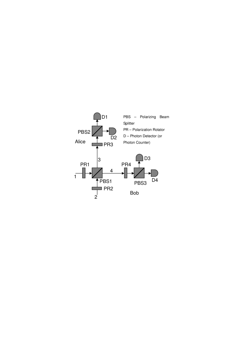
Figure 1: Schematic of a test of LR with the independent photons source. Two spatially and temporally matched polarized photons are inserted at 1 and 2. The polarization rotators PR1 and PR2 are set so that photons 1 and 2 are linearly polarized at equal angles when they reach the polarizing beam splitter PBS1. After PBS1, the photons are in a nonmaximally entangled state [see Eq. (3)] and are sent to Alice’s and Bob’s detector setups. Each detector setup uses a PR, a PBS and two detectors. The PR is used to select measurement bases by rotating the photon’s polarization state.

Consider a pair of photons arriving in modes 1 and 2 of Fig. 1 in the state

$$|\psi\rangle_{12}=|H\rangle_{1}|H\rangle_{2},$$ (1)

where H (V) denotes horizontal (vertical) polarization. We set the polarization rotators PR1 and PR2 to the same angle to produce the state

$$|\psi^{\prime}\rangle_{12}=(\alpha|H\rangle_{1}+\beta|V\rangle_{1})(\alpha|H\rangle_{2}+\beta|V\rangle_{2}),$$ (2)

where $|\alpha|^{2}+|\beta|^{2}=1$. After polarizing beam splitter PBS1, we get the “pseudo-Bell” state

$$|\psi_{\text{pB}}\rangle =\alpha^{2}|H\rangle_{3}|H\rangle_{4}+\beta^{2}|V\rangle_{3}|V\rangle_{4}$$

$$\qquad+\alpha\beta|H\rangle_{3}|V\rangle_{3}+\alpha\beta|H\rangle_{4}|V\rangle_{4}.$$ (3)

Using these states, we can perform a test of LR. Motivated by the result of Eberhard Eberhard (1993), we investigate the possibility of reducing the minimum detection efficiency required to close the detection loophole in a test of LR by changing the values of $\alpha$ and $\beta$ in Eq. (3).

When we set $|\alpha|=|\beta|=1/\sqrt{2}$ in Eq. (3) and condition on coincidence postselection, we may treat the pseudo-Bell state as a maximally entangled state, as in the experiments reported in Refs. Shih and Alley (1988); Ou and Mandel (1988); Kiess et al. (1993). This postselection process discards events where both photons leave PBS1 in the same direction, effectively projecting onto a Bell state. However, the discarded events may create another loophole similar to the detection loophole for tests of LR Kwiat et al. (1994); DeCaro and Garuccio (1994). To close this loophole, the entire pattern of experimental data must be included when evaluating the terms of a Bell inequality Popescu et al. (1997). Here, we also use all data without postselection, but instead of obtaining a violation of a Bell inequality, we quantify the experimental evidence against all local realistic theories by means of measures derived from the KL divergence.

III DATA ANALYSIS METHOD

Contradictions between experimental results and LR are often shown by the violation of a Bell inequality, such as the CHSH inequality Clauser et al. (1969)

$$E(\hat{A}_{1},\hat{B}_{1})-E(\hat{A}_{1},\hat{B}_{2})+E(\hat{A}_{2},\hat{B}_{1})+E(\hat{A}_{2},\hat{B}_{2})\leq 2,$$ (4)

where the terms $E(\hat{A}_{a},\hat{B}_{b})$ are correlations between Alice’s and Bob’s measurements at settings $\hat{A}_{a}$ and $\hat{B}_{b}$, $a,b\in\{1,2\}$. Following this approach, the departure of an experiment’s results from LR is typically given in terms of the number of standard deviations separating the experimental value of the left-hand side of the CHSH inequality from the upper bound of this inequality, which is $2$. Of course, for any finite set of data, there is a small probability that a system governed by LR could also violate the inequality. The standard deviation partially characterizes the measurement uncertainty due to a finite number of trials, but it does not consider the probability that a local realistic system could also violate the inequality. Because such a system’s (non-)violation can have larger standard deviations, the experimental standard deviation may suggest more confidence in rejecting LR than justified. To avoid this problem, we apply a method proposed by van Dam et al. van Dam et al. (2005). In this method, the statistical strength of a test of LR is characterized by the KL divergence from the experimental statistics to the best prediction by local realistic theories. The method is justified by the observation that the confidence at which the experimental data violate LR is closely related to this KL divergence Bahadur (1967).

To better understand the approach based on the KL divergence, it is helpful to analyze tests of LR in terms of a two-player game. The two players are the quantum experimenter QM and the theoretician LRT who wants LR to prevail. During the test of LR, given a source of quantum states, experimenter QM can randomly change the measurement settings. After a large number $N$ of trials, QM obtains empirical frequencies $\mathbf{q}$ of measurement settings and outcomes from the experimental data, which, hopefully, are consistent with the quantum prediction and violate LR. At the same time, knowing the state preparation procedure and the distribution of measurement settings but not the actual settings or outcomes, LRT can design all kinds of different local realistic theories, predicting different probability distributions $\mathbf{p}$ for the settings and outcomes. (We are assuming that state preparation protocols and measurement setting distributions are not changed during the experiment.) The goal is to make $\mathbf{p}$ as consistent as possible with the eventually obtained frequencies $\mathbf{q}$. This requires minimizing a distance between the QM’s frequencies $\mathbf{q}$ and LRT’s prediction $\mathbf{p}$. Following the argument in Ref. van Dam et al. (2005), this distance can be measured by the KL divergence from $\mathbf{q}$ to $\mathbf{p}$, as defined by

$$D_{\text{KL}}(\mathbf{q}\parallel\mathbf{p})=\sum_{k=1}^{K}\sum_{l=1}^{L}q_{kl}\log_{2}\left(\frac{q_{kl}}{p_{kl}}\right),$$ (5)

where $k$ is the measurement setting index, $K$ is the number of different measurement settings, $l$ is the measurement outcome index, and $L$ is the number of different measurement outcomes under each measurement setting. For example, in the test of the CHSH inequality using photon pairs maximally entangled in polarization, $k$ denotes one of the measurement settings $(\hat{A}_{1},\hat{B}_{1})$, $(\hat{A}_{1},\hat{B}_{2})$, $(\hat{A}_{2},\hat{B}_{1})$, or $(\hat{A}_{2},\hat{B}_{2})$, and so $K=2\times 2=4$; $l$ denotes one of the outcomes (H, H), (H, V), (V, H), or (V, V) (assuming perfect detection) and so $L=2\times 2=4$.

The KL divergence has the property that $D_{\text{KL}}(\mathbf{q}\parallel\mathbf{p})\geq 0$, with equality if and only if $\mathbf{p}=\mathbf{q}$. Since there are many different local realistic theories, LRT has the freedom to choose the best one $\mathbf{p}^{(s)}$, namely, the one that minimizes the KL divergence. We can then define a distance from $\mathbf{q}$ to the best local realistic theory according to

$$D_{\text{KL}}(\mathbf{q}\parallel\mathbf{p}^{(s)})=\min_{\mathbf{p}\in\mathit{P}}D_{\text{KL}}(\mathbf{q}\parallel\mathbf{p}),$$ (6)

where $\mathit{P}$ is the set of local realistic theories. Likewise, QM also has the freedom to choose different measurement settings and setting distributions so that the best local realistic theory explains the experimental data poorly. Hence, the general problem is to determine the maximum statistical strength $S$ of tests of LR subject to experimental constraints, which is defined to be

$$S\equiv D_{\text{KL}}\left(\mathbf{q}^{(s)}\parallel\mathbf{p}^{(s)}\right)=\max_{\mathbf{q}\in\mathit{Q}}\min_{\mathbf{p}\in P}D_{\text{KL}}(\mathbf{q}\parallel\mathbf{p}),$$ (7)

where $\mathbf{q}^{(s)}$ is an optimal quantum strategy maximizing Eq. (6), and $\mathit{Q}$ is the set of accessible quantum strategies. The statistical strength is asymptotically related to the $p$-value for rejection of LR. There is a statistical test such that if $S>0$, then for almost all infinite sequences of outcomes of independent experiments, the $p$-value after $N$ experiments is bounded by

$$p_{N}=2^{-NS+o(N)},$$ (8)

where $o(N)$ is a data-dependent term that goes to $0$ as $N\rightarrow\infty$ Bahadur (1967). No statistical test can have a better asymptotic $p$-value. Because $1-p_{N}$ can be thought of as a confidence in rejecting LR, the statistical strength $S$ quantifies the asymptotic rate at which confidence is gained. In particular, the number of experiments required to have reasonable confidence in rejecting LR is necessarily greater than $1/S$.

LRT’s effort to minimize the KL divergence as in Eq. (6) is a maximum likelihood estimation problem. Here, we use the expectation-maximization algorithm in Ref. Vardi and Lee (1993). The general problem of computing the statistical strength $S$ is nontrivial. To calculate $S$, we maximize Eq. (6) over measurement settings with standard nonlinear optimization techniques.

To calculate the statistical strength of a test of LR, we need to learn how LRT predicts the measurement results given the state preparation procedure and possible measurement settings. Suppose that for a bipartite system with $n_{A}\times n_{B}$ measurement settings there are $d_{A}$ outcomes for each of $n_{A}$ measurement settings at Alice’s side, and there are $d_{B}$ outcomes for each of $n_{B}$ measurement settings at Bob’s side. Then the local realistic description implies the existence of a single joint probability distribution over a $d_{A}^{n_{A}}\times d_{B}^{n_{B}}$-element event space, which we write as

$$P_{\text{LR}}\left(a_{1},\ldots,a_{n_{A}};b_{1},\ldots,b_{n_{B}}|\hat{A}_{1},\ldots,\hat{A}_{n_{A}};\hat{B}_{1},\ldots,\hat{B}_{n_{B}}\right),$$ (9)

where $a_{1},\ldots,a_{n_{A}}\in\{1,2,\ldots,d_{A}\}$, and $b_{1},\ldots,b_{n_{B}}\in\{1,2,\ldots,d_{B}\}$, with normalization

$$\sum_{a_{1},\ldots,a_{n_{A}}=1}^{d_{A}}\hskip 14.22636pt\sum_{b_{1},\ldots,b_{n_{B}}=1}^{d_{B}}P_{\text{LR}}\left(a_{1},\ldots,a_{n_{A}};b_{1},\ldots,b_{n_{B}}|\hat{A}_{1},\ldots,\hat{A}_{n_{A}};\hat{B}_{1},\ldots,\hat{B}_{n_{B}}\right)=1$$ (10)

Hence, the marginal probability for the measurement outcome ($a_{i}$; $b_{j}$) when settings $\hat{A}_{i}$ and $\hat{B}_{j}$ are chosen is given by

$$P_{\text{LR}}(a_{i};b_{j}|\hat{A}_{i};\hat{B}_{j}) =\sum_{a_{1},\ldots,a_{i-1},a_{i+1},\ldots,a_{n_{A}}=1}^{d_{A}}\hskip 14.22636pt\sum_{b_{1},\ldots,b_{j-1},b_{j+1},\ldots,b_{n_{B}}=1}^{d_{B}}\hskip 113.81102pt$$

$$\qquad\hskip 56.9055ptP_{\text{LR}}\left(a_{1},\ldots,a_{n_{A}};b_{1},\ldots,b_{n_{B}}|\hat{A}_{1},\ldots,\hat{A}_{n_{A}};\hat{B}_{1},\ldots,\hat{B}_{n_{B}}\right).$$ (11)

Since the probabilities $P_{\text{LR}}(a_{i};b_{j}|\hat{A}_{i};\hat{B}_{j})$ are constrained to be marginal distributions, they satisfy nontrivial relationships. The goal of a test of LR is to choose states and settings that result in quantum predictions that cannot be obtained as the marginals of a single local realistic theory for all $i$ and $j$. The quantum-mechanical prediction of the probability is given by $P_{\text{qm}}(a_{i};b_{j}|\hat{A}_{i};\hat{B}_{j})=\text{Tr}(\rho O(a_{i};b_{j}|\hat{A}_{i};\hat{B}_{j}))$, where $\rho$ is the density matrix of the quantum state, and $O(a_{i};b_{j}|\hat{A}_{i};\hat{B}_{j})$ is the positive operator valued measure (POVM) element corresponding to the measurement outcome ($a_{i}$; $b_{j}$) when Alice and Bob use settings $\hat{A}_{i}$ and $\hat{B}_{j}$, respectively. Given the distributions of measurement settings chosen by Alice and Bob, the KL divergence measures the statistical distance of the optimal local realistic theory from the quantum predictions as in Eq. (6).

IV Results and Discussion

We consider tests of LR using the independent inputs source for pseudo-Bell pairs and tests using unbalanced Bell pairs. In both cases, Alice and Bob use measurement devices like those shown in Fig. 1. They use either counters or detectors for photon detection, and they independently and uniformly randomly choose one of two measurement settings each, where the settings are determined by the polarization rotators. We use Bloch-sphere Euler angles as explained below to define the measurement settings. We label the measurement settings $\hat{A}_{1}$ and $\hat{A}_{2}$ (Alice) or $\hat{B}_{1}$ and $\hat{B}_{2}$ (Bob) and write the two-photon state coming in at modes 3 and 4 in Fig. 1 as $|\psi\rangle_{AB}$. We calculate the statistical strength $S$ according to Eq. (7) by maximizing over the angles of the measurement settings $\{\hat{A}_{1},\hat{A}_{2},\hat{B}_{1},\hat{B}_{2}\}$ and minimizing over the set of local realistic theories $\mathit{P}$, where we fix the two-photon state $|\psi\rangle_{AB}$ shared by Alice and Bob. The inner minimization as implemented guarantees convergence to the optimum $\mathbf{p}^{(s)}$, whereas the outer one obtains a local optimum. Confidence in global optimality can be obtained by repetition from many different starting points (which we have done) or more sophisticated search strategies. A local optimum satisfying $S>0$ is sufficient for having found a detection-loophole-free test. On the other hand, finding no solution with $S>0$ is heuristic evidence that such a test does not exist subject to the constraints of the experiment. Thus, with this optimization strategy, we can trace the boundary of the region for which $S>0$ (by searching for where $S$ decreases to $0$) to heuristically determine the minimum detection efficiency $\eta_{\text{min}}$ and the associated optimal measurement settings $\{\hat{A}_{\text{1min}},\hat{A}_{\text{2min}},\hat{B}_{\text{1min}},\hat{B}_{\text{2min}}\}$ needed to perform a test of LR of this type free of the detection loophole with a given state.

Note that as $S\to 0$, the number of experiments required to gain confidence close to unity diverges. For a constant rate of gaining confidence [see the explanation below Eq. (8)], we set the desired statistical strength $S=X>0$ and determine the minimum detection efficiency $\eta_{c}$ and the associated optimal measurement settings $\{\hat{A}_{1c},\hat{A}_{2c},\hat{B}_{1c},\hat{B}_{2c}\}$ that achieve statistical strength $X$. The strategy for finding such solutions $\{\eta_{c},\hat{A}_{1c},\hat{A}_{2c},\hat{B}_{1c},\hat{B}_{2c}\}$ is as follows: First we start with a set of solutions $\{\eta_{\text{old}},\hat{A}_{\text{1old}},\hat{A}_{\text{2old}},\hat{B}_{\text{1old}},\hat{B}_{\text{2old}}\}$ having statistical strength $X_{\text{old}}\geq X$. Second we optimize Eq. (6) over the measurement settings $\{\hat{A}_{1},\hat{A}_{2},\hat{B}_{1},\hat{B}_{2}\}$ with fixed detection efficiency $\eta_{\text{old}}$, which yields new settings $\{\hat{A}_{\text{1new}},\hat{A}_{\text{2new}},\hat{B}_{\text{1new}},\hat{B}_{\text{2new}}\}$ achieving $S=Y$ ($Y\geq X_{\text{old}}$) for efficiency $\eta_{\text{old}}$. Third, we decrease the detection efficiency from $\eta_{\text{old}}$ to $\eta_{\text{new}}$ as much as we can without reducing the statistical strength to below $X$, so that this new set of solutions $\{\eta_{\text{new}},\hat{A}_{\text{1new}},\hat{A}_{\text{2new}},\hat{B}_{\text{1new}},\hat{B}_{\text{2new}}\}$ has $S=X_{\text{new}}$ with $X_{\text{new}}$ close to $X$ (within numerical error). We then repeat the above procedure several times replacing the old with the new solutions, until we are unable to reduce the efficiency parameter. We thus find heuristically optimal solutions $\{\eta_{c},\hat{A}_{1c},\hat{A}_{2c},\hat{B}_{1c},\hat{B}_{2c}\}$.

Table 1: Extreme conditions for tests of LR free of the detection loophole for photon counters or photon detectors using the unbalanced Bell states $|\psi_{\text{uB}}\rangle$ defined in Eq. (12). The asymptotic behavior when $\theta\to 0$ is consistent with results in Ref. Vertesi et al. (2009), which are shown in the last row. The angle parameters are explained in the text.

$\theta$	$\alpha_{\text{1min}}$	$\alpha_{\text{2min}}$	$\beta_{\text{1min}}$	$\beta_{\text{2min}}$	$\eta_{\text{min}}$
$45^{\circ}$	$22.50^{\circ}$	$-67.50^{\circ}$	$-22.50^{\circ}$	$67.50^{\circ}$	$82.85\,\%$
$40^{\circ}$	$21.28^{\circ}$	$-66.89^{\circ}$	$-21.28^{\circ}$	$66.89^{\circ}$	$80.61\,\%$
$35^{\circ}$	$19.40^{\circ}$	$-65.60^{\circ}$	$-19.40^{\circ}$	$65.60^{\circ}$	$78.50\,\%$
$30^{\circ}$	$17.00^{\circ}$	$-63.58^{\circ}$	$-17.00^{\circ}$	$63.58^{\circ}$	$76.50\,\%$
$25^{\circ}$	$14.21^{\circ}$	$-60.72^{\circ}$	$-14.21^{\circ}$	$60.72^{\circ}$	$74.60\,\%$
$20^{\circ}$	$11.14^{\circ}$	$-56.79^{\circ}$	$-11.14^{\circ}$	$56.79^{\circ}$	$72.81\,\%$
$15^{\circ}$	$7.92^{\circ}$	$-51.42^{\circ}$	$-7.92^{\circ}$	$51.42^{\circ}$	$71.12\,\%$
$10^{\circ}$	$4.70^{\circ}$	$-43.88^{\circ}$	$-4.70^{\circ}$	$43.88^{\circ}$	$69.53\,\%$
$5^{\circ}$	$1.81^{\circ}$	$-32.41^{\circ}$	$-1.81^{\circ}$	$32.41^{\circ}$	$68.06\,\%$
$4^{\circ}$	$1.32^{\circ}$	$-29.25^{\circ}$	$-1.32^{\circ}$	$29.25^{\circ}$	$67.78\,\%$
$3^{\circ}$	$0.87^{\circ}$	$-25.55^{\circ}$	$-0.87^{\circ}$	$25.55^{\circ}$	$67.52\,\%$
$2^{\circ}$	$0.48^{\circ}$	$-21.04^{\circ}$	$-0.48^{\circ}$	$21.04^{\circ}$	$67.27\,\%$
$1^{\circ}$	$0.17^{\circ}$	$-15.01^{\circ}$	$-0.17^{\circ}$	$15.01^{\circ}$	$67.06\,\%$
$\to 0$	$0$	$\to-2\theta^{1/2}$	$0$	$\to 2\theta^{1/2}$	$\to 2/3$

First, we analyze unbalanced Bell states of the form

$$|\psi_{\text{uB}}\rangle=\cos(\theta)|H\rangle_{A}|H\rangle_{B}+\sin(\theta)|V\rangle_{A}|V\rangle_{B},$$ (12)

where $\theta\in(0,\pi/4]$. Note that whether there is a relative phase $e^{i\Delta\phi}$ between the second and first terms of Eq. (12) is not important, since Alice can always adjust her polarization basis, i.e., $|H\rangle_{A}\to|H\rangle_{A}$, and $|V\rangle_{A}\to e^{-i\Delta\phi}|V\rangle_{A}$, to put the state in the above form. In principle, the state $|\psi_{\text{uB}}\rangle$ can be simulated by postselection on the state $|\psi_{\text{pB}}\rangle$ [Eq. (3)], although this introduces a loophole as mentioned earlier. Experimental techniques to prepare $|\psi_{\text{uB}}\rangle$ without postselection have been demonstrated and applied to tests of LR White et al. (1999); Brida et al. (2000). Here we calculate the statistical strength for photon detectors. Photon counters have no advantage over photon detectors here, because no more than one photon arrives at Alice’s or Bob’s detectors. That is, counters and detectors have the same possibilities for detection outcomes and with the same probabilities. Our optimization results are summarized in Table 1 and Fig. 2. The measurement angle $\alpha_{i,\,\text{min}}$ (or $\beta_{j,\,\text{min}}$) shown in Table 1 is the angle from the $z$ axis of the polarization state of an incoming photon that gets reflected at PBS2 (or PBS3) in Fig. 1, where we use the Bloch sphere representation for this state. By convention, $|H\rangle$ and $\frac{1}{\sqrt{2}}(|H\rangle+|V\rangle)$ are polarization states associated with the $z$ and $x$ axes, respectively. In general, we let the “unhatted” form of the measurement setting denote twice the traceless part of this reflected state’s density matrix, or equivalently, the measurement operator that describes the effect of the PR, PBS and ideal detector combination on single photon states. For example, $A_{ic}=\cos(\alpha_{ic})\sigma_{z}+\sin(\alpha_{ic})[\cos(\phi_{ic})\sigma_{x}+\sin(\phi_{ic})\sigma_{y}]$. The optimizations show heuristically that we can take $\phi_{ic}=0$ everywhere; i.e., all the optimal measurement settings lie in the $(x,z)$ plane of the Bloch sphere, an observation which has been proven for several special cases Gisin (1991); Popescu and Rohrlich (1992); Scarani and Gisin (2001).

From Table 1, we can see that when the statistical strength $S$ approaches $0$, $\alpha_{i,\,\text{min}}=-\beta_{i,\,\text{min}}$ for $i=1,2$. The minimum detection efficiency $\eta_{\text{min}}$ decreases monotonically with the parameter $\theta$ in $|\psi_{\text{uB}}\rangle$ and is $82.85\,\%$ when $\theta=\pi/4$, where the state is a Bell state. It approaches $2/3$ when $\theta$ approaches $0$, where the state is very close to a product state. These results are consistent with previous results Garg and Mermin (1987); Eberhard (1993). From Fig. 2, we can see how the optimal statistical strength increases for $\eta>\eta_{\text{min}}$ and how the input state must change to achieve this statistical strength. Note that not all unbalanced Bell states can achieve a given statistical strength level $S>0$, even for $\eta=1$. For example, for $S\geq 10^{-4}$, the parameter $\theta$ must be greater than $0.98^{\circ}$. Associated measurement settings can be found in the tables in the appendix.

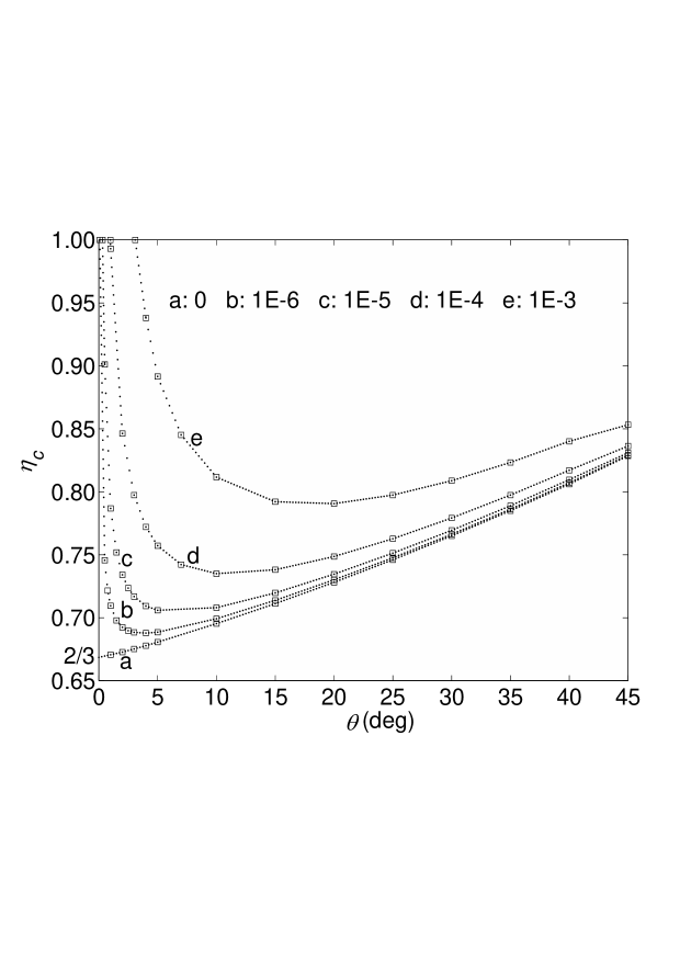
Figure 2: Detection efficiency of photon counters or photon detectors required for different statistical strength levels $S$ vs the parameter $\theta$ [Eq. (12)]. The empty squares show our calculated points, and the dotted lines are linear interpolations to guide the eyes. In curve a, the linear extrapolation toward $\theta=0$ is shown.

We now consider the pseudo-Bell states of Eq. (3). Let $\alpha=\cos(\gamma)$ and $\beta=\sin(\gamma)e^{i\phi}$, then Eq. (3) can be rewritten as

$$|\psi_{\text{pB}}\rangle =\cos^{2}(\gamma)|H\rangle_{3}|H\rangle_{4}+\sin^{2}(\gamma)e^{i2\phi}|V\rangle_{3}|V\rangle_{4}$$

$$\qquad+\cos(\gamma)\sin(\gamma)e^{i\phi}(|H\rangle_{3}|V\rangle_{3}+|H\rangle_{4}|V\rangle_{4}),$$ (13)

where $\gamma\in(0,\pi/4]$, and $\phi\in[0,2\pi)$. We can prepare different pseudo-Bell states by changing the values of both $\gamma$ and $\phi$. However, for a given $\gamma$, as the following discussion shows, the optimal statistical strength $S$ is the same regardless of the value of $\phi$. In the test of LR as shown in Fig. 1, Alice’s and Bob’s measurements are restricted to polarization rotation followed by photon counting. They cannot detect coherences between any two of the first two, the third, and the last terms in the state $|\psi_{\text{pB}}\rangle$ as written in Eq. (13), because these terms correspond to different photon-number-distribution subspaces. Hence, the measurement outcomes determined by $|\psi_{\text{pB}}\rangle$ are equivalent to the outcomes given by a mixture of the following two states:

$$|\psi_{1}\rangle\langle\psi_{1}|,\;\textrm{with}\;|\psi_{1}\rangle\propto\cos^{2}(\gamma)|H\rangle_{3}|H\rangle_{4}+\sin^{2}(\gamma)e^{i2\phi}|V\rangle_{3}|V\rangle_{4},$$ (14)

and

$$\rho_{2}\propto|H\rangle_{3}|V\rangle_{3}\hskip 5.69046pt{}_{3}\langle H|_{3}\langle V|+|H\rangle_{4}|V\rangle_{4}\hskip 5.69046pt{}_{4}\langle H|_{4}\langle V|.$$ (15)

Since the state $|\psi_{1}\rangle$ can be written in the form $|\psi_{\text{uB}}\rangle$ as in Eq. (12) by changing the mode labels and the state bases, the measurement outcomes attributable to $|\psi_{1}\rangle$ can reveal a violation of LR when $\gamma\in(0,\pi/4]$, as our earlier results show. But $\rho_{2}$ is a separable state and so the outcomes attributable to $\rho_{2}$ can be explained by LR no matter what the measurement settings $\{\hat{A}_{1},\hat{A}_{2},\hat{B}_{1},\hat{B}_{2}\}$ are. Hence, in a test of LR, the information about whether LR is or is not violated is conveyed only by the outcomes from $|\psi_{1}\rangle$, while the state $\rho_{2}$ acts as noise. Based on these considerations and the earlier arguments about being able to eliminate a potential phase in $|\psi_{\text{uB}}\rangle$, we do not need to consider different phases $\phi$ in the pseudo-Bell state $|\psi_{\text{pB}}\rangle$ when calculating the optimal statistical strength $S$, so we can choose a fixed value, such as $\phi=0$. Moreover, we determined heuristically by extended optimizations in selected cases that the optimal measurement settings $\{\hat{A}_{1c},\hat{A}_{2c},\hat{B}_{1c},\hat{B}_{2c}\}$ can be chosen to lie in the $(x,z)$ plane of the Bloch sphere, just like for $|\psi_{\text{uB}}\rangle$. Taking these observations into account reduces the number of free parameters and speeds up the general calculations.

The optimization results for pseudo-Bell states are summarized in Table 2 and Fig. 3. Similar to unbalanced Bell states, Table 2 shows that when the statistical strength $S$ approaches $0$, $\alpha_{i,\,\text{min}}=-\beta_{i,\,\text{min}}$ for $i=1,2$. Figure 3 shows that there is a lower bound on the state parameter $\gamma$ to achieve a nonzero statistical strength level $S$. Measurement settings for the data shown in Fig. 3 are given in the appendix.

Table 2: Extreme conditions for tests of LR free of the detection loophole for photon counters and photon detectors using the pseudo-Bell states of Eq. (13). The angle parameters are explained in the text.

	Photon counter					Photon detector
$\gamma$	$\alpha_{\text{1min}}$	$\alpha_{\text{2min}}$	$\beta_{\text{1min}}$	$\beta_{\text{2min}}$	$\eta_{\text{min}}$	$\alpha_{\text{1min}}$	$\alpha_{\text{2min}}$	$\beta_{\text{1min}}$	$\beta_{\text{2min}}$	$\eta_{\text{min}}$
$45^{\circ}$	$22.50^{\circ}$	$-67.50^{\circ}$	$-22.50^{\circ}$	$67.50^{\circ}$	$90.62\,\%$	$11.64^{\circ}$	$-63.88^{\circ}$	$-11.64^{\circ}$	$63.88^{\circ}$	$92.23\,\%$
$40^{\circ}$	$20.49^{\circ}$	$-66.01^{\circ}$	$-20.49^{\circ}$	$66.01^{\circ}$	$89.71\,\%$	$11.08^{\circ}$	$-62.79^{\circ}$	$-11.08^{\circ}$	$62.79^{\circ}$	$91.31\,\%$
$35^{\circ}$	$16.76^{\circ}$	$-62.14^{\circ}$	$-16.76^{\circ}$	$62.14^{\circ}$	$89.78\,\%$	$9.79^{\circ}$	$-59.60^{\circ}$	$-9.79^{\circ}$	$59.60^{\circ}$	$91.11\,\%$
$30^{\circ}$	$12.32^{\circ}$	$-56.16^{\circ}$	$-12.32^{\circ}$	$56.16^{\circ}$	$90.80\,\%$	$7.93^{\circ}$	$-54.42^{\circ}$	$-7.93^{\circ}$	$54.42^{\circ}$	$91.71\,\%$
$25^{\circ}$	$8.00^{\circ}$	$-48.43^{\circ}$	$-8.00^{\circ}$	$48.43^{\circ}$	$92.57\,\%$	$5.73^{\circ}$	$-47.46^{\circ}$	$-5.73^{\circ}$	$47.46^{\circ}$	$93.05\,\%$
$20^{\circ}$	$4.43^{\circ}$	$-39.49^{\circ}$	$-4.43^{\circ}$	$39.49^{\circ}$	$94.71\,\%$	$3.53^{\circ}$	$-39.09^{\circ}$	$-3.53^{\circ}$	$39.09^{\circ}$	$94.89\,\%$
$15^{\circ}$	$1.96^{\circ}$	$-29.88^{\circ}$	$-1.96^{\circ}$	$29.88^{\circ}$	$96.81\,\%$	$1.68^{\circ}$	$-29.76^{\circ}$	$-1.68^{\circ}$	$29.76^{\circ}$	$96.85\,\%$
$10^{\circ}$	$0.59^{\circ}$	$-19.98^{\circ}$	$-0.59^{\circ}$	$19.98^{\circ}$	$98.52\,\%$	$0.54^{\circ}$	$-19.96^{\circ}$	$-0.54^{\circ}$	$19.96^{\circ}$	$98.53\,\%$
$5^{\circ}$	$0.07^{\circ}$	$-10.00^{\circ}$	$-0.07^{\circ}$	$10.00^{\circ}$	$99.63\,\%$	$0.07^{\circ}$	$-10.00^{\circ}$	$-0.07^{\circ}$	$10.00^{\circ}$	$99.63\,\%$

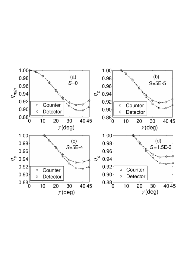
Figure 3: Detection efficiencies of photon counters and photon detectors required for different statistical strength levels $S$ vs the parameter $\gamma$ of the pseudo-Bell state of Eq. (13): (a) $S=0$, (b) $S=$ 5E-5, (c) $S=$ 5E-4, and (d) $S=$ 1.5E-3. The calculated points are labeled by squares for photon counters and by diamonds for photon detectors, and the dotted lines are linear interpolations to guide the eyes.

Table 2 and Fig. 3 (a) show that the minimum detection efficiency $\eta_{\text{min}}$ required to close the detection loophole achieves its minimum in the interior of the domain, in contrast to what was found for the case of unbalanced Bell states. We might have expected this behavior based on the following observations: First, with respect to the detector setups used, the state $|\psi_{\text{pB}}\rangle$ can be thought of as the state $|\psi_{\text{uB}}\rangle$ with noise, as pointed out above, and second, the violation of LR given by $|\psi_{\text{uB}}\rangle$ is very sensitive to noise, particularly when $\theta$ [Eq. (12)] is small Brunner et al. (2007). Figure 3 (a) also suggests that any pseudo-Bell state $|\psi_{\text{pB}}\rangle$ can violate LR using counters or detectors with sufficient efficiency.

When we look at the minimum detection efficiency required to achieve a given statistical strength level $S$, the efficiencies of photon counters and photon detectors are notably different, showing the utility of the additional information available with photon counters. The advantage of photon counters is most notable for $\gamma$ between approximately $35^{\circ}$ and $45^{\circ}$. In particular, the minimum detection efficiency $\eta_{\text{min}}$ is $89.71\,\%$ for photon counters and $91.11\,\%$ for photon detectors and is achieved for $\gamma$ in this range. Loosely speaking, this advantage is because photon counters are better at differentiating between measurement outcomes contributed by the entangled ($|\psi_{1}\rangle$) and unentangled ($\rho_{2}$) parts of the state $|\psi_{\text{pB}}\rangle$.

A comparison of Figs. 2 and 3 suggests that higher efficiencies are required to achieve given statistical strengths with $|\psi_{\text{pB}}\rangle$ than with $|\psi_{\text{uB}}\rangle$. This again can be attributed to the noise added by $\rho_{2}$ to measurement outcomes, which reduces the statistical strength considerably. As an explicit example, consider the optimal statistical strengths $S^{(1)}$ or $S^{(2)}$ achievable with

$$|\psi_{\text{uB}}(\theta=\pi/4)\rangle=\frac{1}{\sqrt{2}}(|H\rangle_{A}|H\rangle_{B}+|V\rangle_{A}|V\rangle_{B}),$$ (16)

or with

$$|\psi_{\text{pB}}(\gamma=\pi/4,\phi=0)\rangle=\frac{1}{2}(|H\rangle_{3}|H\rangle_{4}+|V\rangle_{3}|V\rangle_{4}+|H\rangle_{3}|V\rangle_{3}+|H\rangle_{4}|V\rangle_{4}).$$ (17)

We find that $S^{(1)}=2S^{(2)}\approx 0.04627$ for perfect photon counters. The ratio can be explained by observing that half of the measurement outcomes of $|\psi_{\text{pB}}(\gamma=\pi/4,\phi=0)\rangle$ are from the separable $\rho_{2}$.

V Conclusion

We have demonstrated a method to measure the statistical strength of tests of LR that is based on the KL divergence from the predicted experimental frequencies to the best prediction given by LR. This method helps to design a loophole-free test of LR and quantifies the confidence in violation of LR for sufficiently large experimental data sets. We used the method to determine optimal statistical strengths of tests of LR using a typical detector setup for polarized photon pairs with inefficient detectors. We considered both ideal unbalanced Bell states and pseudo-Bell states obtained by combining independent polarized photons on a polarizing beam splitter. Creating the latter can be easier Shih and Alley (1988); Ou and Mandel (1988); Kiess et al. (1993), but observing a violation of LR requires higher detection efficiencies. Our calculations show that with pseudo-Bell states, we can close the detection loophole with a minimum detection efficiency of $89.71\,\%$ using photon counters, or $91.11\,\%$ using photon detectors. For unbalanced Bell states, we confirmed previous calculations Eberhard (1993) showing that violations of LR are possible at detection efficiencies above $2/3$. Furthermore, we numerically exhibited the relationships between state parameters and minimum detection efficiencies needed to achieve given levels of statistical strength. Given that the current roadblock for performing loophole-free tests of LR with photons is detection inefficiency rather than the difficulty of obtaining an entangled source, we cannot recommend using the pseudo-Bell state for such an experiment.

In current experiments based on spontaneous parametric down-conversion to produce entangled photon pairs, we must consider other sources of potentially unwanted measurement outcomes. Such sources include dark counts and the generation of more than one photon pair Wasilewski et al. (2006); Lvovsky et al. (2007). The latter effect can be quite noticeable, particularly for the brighter, more strongly pumped sources. Further work is required to analyze the consequences of these effects for statistical strength. It is also desirable to obtain rigorous confidence levels for the rejection of LR with moderately sized data sets. Such levels could improve on measures derived from experimental standard deviations of Bell-inequality violation.

*

Appendix A Optimization results

Using code written in Octave , which is available by request, we find the results as shown in the following tables. In these tables, the units of the columns labeled theta, gamma, A_1, A_2, B_1, and B_2 are degrees ($\circ$). The column labeled theta (or gamma) contains the values of the parameter $\theta$ in the state $|\psi_{\text{uB}}\rangle=\cos(\theta)|H\rangle_{A}|H\rangle_{B}+\sin(\theta)|V\rangle_{A}|V\rangle_{B}$ (or the value of the parameter $\gamma$ in the state $|\psi_{\text{pB}}\rangle=\cos^{2}(\gamma)|H\rangle_{3}|H\rangle_{4}+\sin^{2}(\gamma)|V\rangle_{3}|V\rangle_{4}+\cos(\gamma)\sin(\gamma)(|H\rangle_{3}|V\rangle_{3}+|H\rangle_{4}|V\rangle_{4})$). The columns labeled A_1 and A_2 contain the two optimal measurement setting angles for Alice, while the columns labeled B_1 and B_2 contain the two optimal measurement setting angles for Bob. The columns labeled eta_1 and eta_2 give the detection efficiencies required to achieve the statistical strengths in the columns labeled S_1 and S_2, respectively. Due to limits of numerical accuracy, we cannot find the exact detection efficiency $\eta_{c}$ required to achieve a specified statistical strength level $S$. Up to the $10^{-4}$ level, we list the best two detection efficiencies, which are closest to $\eta_{c}$. Using eta_1, the statistical strength of a test of LR is a little higher than the specified level, while using eta_2, the statistical strength is a little lower than the specified level. In the plots of Fig. 2 and Fig. 3, we use eta_1 or eta_2, according to which of them gives a statistical strength closer to the specified level. Also, for calculations of the minimum detection efficiency at $0+\epsilon$ statistical strength, we truncate the statistical strength to $0$ when it is numerically calculated to be less than $10^{-9}$ or $10^{-10}$, depending on the situation.

A.1 Results for states $|\psi_{\text{uB}}\rangle=\cos(\theta)|H\rangle_{A}|H\rangle_{B}+\sin(\theta)|V\rangle_{A}|V\rangle_{B}$ using photon counters or photon detectors

unbalancedBellstates.txt

A.2 Results for states $|\psi_{\text{pB}}\rangle=\cos^{2}(\gamma)|H\rangle_{3}|H\rangle_{4}+\sin^{2}(\gamma)|V\rangle_{3}|V\rangle_{4}+\cos(\gamma)\sin(\gamma)(|H\rangle_{3}|V\rangle_{3}+|H\rangle_{4}|V\rangle_{4})$ using photon counters

photoncounter.txt

A.3 Results for states $|\psi_{\text{pB}}\rangle=\cos^{2}(\gamma)|H\rangle_{3}|H\rangle_{4}+\sin^{2}(\gamma)|V\rangle_{3}|V\rangle_{4}+\cos(\gamma)\sin(\gamma)(|H\rangle_{3}|V\rangle_{3}+|H\rangle_{4}|V\rangle_{4})$ using photon detectors

photondetector.txt

References

- Bell (1964) J. S. Bell, Physics 1, 195 (1964).
- Peres (1999) A. Peres, Found. Phys. 29, 589 (1999).
- Werner and Wolf (2001) R. F. Werner and M. M. Wolf, Quant. Inf. Comp. 1, 1 (2001).
- Horodecki et al. (2009) R. Horodecki, P. Horodecki, M. Horodecki, and K. Horodecki, Rev. Mod. Phys. 81, 865 (2009).
- Clauser et al. (1969) J. F. Clauser, M. A. Horne, A. Shimony, and R. A. Holt, Phys. Rev. Lett. 23, 880 (1969).
- Freedman and Clauser (1972) S. J. Freedman and J. F. Clauser, Phys. Rev. Lett. 28, 938 (1972).
- Genovese (2005) M. Genovese, Phys. Rep. 413, 319 (2005).
- Pearle (1970) P. M. Pearle, Phys. Rev. D 2, 1418 (1970).
- Bell (2004) J. S. Bell, Speakable and Unspeakable in Quantum Mechanics (Cambridge University Press, Cambridge, 2004), pp. 139-158.
- Garg and Mermin (1987) A. Garg and N. D. Mermin, Phys. Rev. D 35, 3831 (1987).
- Eberhard (1993) P. H. Eberhard, Phys. Rev. A 47, R747 (1993).
- Larsson and Semitecolos (2001) J.-A. Larsson and J. Semitecolos, Phys. Rev. A 63, 022117 (2001).
- Cabello and Larsson (2007) A. Cabello and J.-A. Larsson, Phys. Rev. Lett. 98, 220402 (2007).
- Brunner et al. (2007) N. Brunner, N. Gisin, V. Scarani, and C. Simon, Phys. Rev. Lett. 98, 220403 (2007).
- Rowe et al. (2001) M. A. Rowe, D. Kielpinski, V. Meyer, C. A. Sackett, W. M. Itano, C. Monroe, and D. J. Wineland, Nature 409, 791 (2001).
- Aspect et al. (1982) A. Aspect, J. Dalibard, and G. Roger, Phys. Rev. Lett. 49, 1804 (1982).
- Weihs et al. (1998) G. Weihs, T. Jennewein, C. Simon, H. Weinfurter, and A. Zeilinger, Phys. Rev. Lett. 81, 5039 (1998).
- Tittel et al. (1999) W. Tittel, J. Brendel, N. Gisin, and H. Zbinden, Phys. Rev. A 59, 4150 (1999).
- Barrett et al. (2005) J. Barrett, L. Hardy, and A. Kent, Phys. Rev. Lett. 95, 010503 (2005).
- Masanes et al. (2009) L. Masanes, R. Renner, A. Winter, J. Barrett, and M. Christandl (2009), eprint arXiv:quant-ph/0606049v4.
- Masanes (2009) L. Masanes, Phys. Rev. Lett. 102, 140501 (2009).
- Lita et al. (2008) A. E. Lita, A. J. Miller, and S. W. Nam, Opt. Express 16, 3032 (2008).
- Shih and Alley (1988) Y. H. Shih and C. O. Alley, Phys. Rev. Lett. 61, 2921 (1988).
- Ou and Mandel (1988) Z. Y. Ou and L. Mandel, Phys. Rev. Lett. 61, 50 (1988).
- Kiess et al. (1993) T. E. Kiess, Y. H. Shih, A. V. Sergienko, and C. O. Alley, Phys. Rev. Lett. 71, 3893 (1993).
- Lounis and Orrit (2005) B. Lounis and M. Orrit, Rep. Prog. Phys. 68, 1129 (2005).
- Oxborrow and Sinclair (2005) M. Oxborrow and A. G. Sinclair, Contemp. Phys. 46, 173 (2005).
- van Dam et al. (2005) W. van Dam, R. D. Gill, and P. D. Grunwald, IEEE Trans. Inf. Theory 51, 2812 (2005).
- Kwiat et al. (1994) P. G. Kwiat, P. H. Eberhard, A. M. Steinberg, and R. Y. Chiao, Phys. Rev. A 49, 3209 (1994).
- DeCaro and Garuccio (1994) L. DeCaro and A. Garuccio, Phys. Rev. A 50, R2803 (1994).
- Popescu et al. (1997) S. Popescu, L. Hardy, and M. Zukowski, Phys. Rev. A 56, R4353 (1997).
- Bahadur (1967) R. R. Bahadur, in Proc. Fifth Berkeley Symp. on Math. Statist. and Prob. (Univ. of Calif. Press, 1967), vol. 1, pp. 13–26.
- Vardi and Lee (1993) Y. Vardi and D. Lee, J. Royal Stat. Soc. B 55, 569 (1993).
- Vertesi et al. (2009) T. Vertesi, S. Pironio, and N. Brunner (2009), eprint arXiv:0909.3171v2 [quant-ph].
- White et al. (1999) A. G. White, D. F. V. James, P. H. Eberhard, and P. G. Kwiat, Phys. Rev. Lett. 83, 3103 (1999).
- Brida et al. (2000) G. Brida, M. Genovese, C. Novero, and E. Predazzi, Phys. Lett. A 268, 12 (2000).
- Gisin (1991) N. Gisin, Phys. Lett. A 154, 201 (1991).
- Popescu and Rohrlich (1992) S. Popescu and D. Rohrlich, Phys. Lett. A 166, 293 (1992).
- Scarani and Gisin (2001) V. Scarani and N. Gisin, J. Phys. A: Math. Gen. 34, 6043 (2001).
- Wasilewski et al. (2006) W. Wasilewski, A. I. Lvovsky, K. Banaszek, and C. Radzewicz, Phys. Rev. A 73, 063819 (2006).
- Lvovsky et al. (2007) A. I. Lvovsky, W. Wasilewski, and K. Banaszek, J. Mod. Optics 54, 721 (2007).