Domain wall propagation due to the synchronization with circularly polarized microwaves

Abstract

Finding a new control parameter for magnetic domain wall (DW) motion in magnetic nanostructures is important in general and in particular for the spintronics applications. Here, we show that a circularly polarized magnetic field (CPMF) at GHz frequency (microwave) can efficiently drive a DW to propagate along a magnetic nanowire. Two motion modes are identified: rigid-DW propagation at low frequency and oscillatory propagation at high frequency. Moreover, DW motion under a CPMF is equivalent to the DW motion under a uniform spin current in the current perpendicular to the plane magnetic configuration proposed recently by Khvalkovskiy et al. [Phys. Rev. Lett. 102, 067206 (2009)], and the CPMF frequency plays the role of the current.

Controlled manipulation of magnetic domain-wall (DW) propagation in nanowires has spurred intensive research in recent yearsWalker ; Cowburn ; Erskine ; xrw ; Slon ; szhang ; szhang1 ; Fert ; Parkin1 ; Parkin2 ; Li ; Khvalkovskiy in nano-magnetism because of its fundamental interest and the potential impact in spintronic device technology. Both static magnetic fieldsWalker ; Cowburn ; Erskine ; xrw and electric currentsSlon ; szhang ; szhang1 ; Fert ; Parkin1 ; Parkin2 ; Li ; Khvalkovskiy can be the control parameters. However, their control mechanisms are different, and they have different advantages and disadvantages. Thus, finding any new control parameter for DW motion should be of great interest.

Although it is known both theoreticallyZZSun and experimentallyXiao that a microwave can be used to manipulate the motion of single domain magnetic particles (macrospins or Stoner particles), a microwave was hardly thought to be an effective control parameter for DW motion. In this letter, we show that a circularly polarized magnetic field (CPMF) at GHz frequency (microwave) can efficiently drive a magnetic DW to propagate along a nanowire at a high speed. Similar to a spin-polarized current, a CPMF can generate both Slonczewski-like and field-like spin-transfer torques (STTs) inside a DW. Unlike the STTs generated by a spin-polarized current, the field-like STT is much bigger than the Slonczewski-like STT. Thus, a CPMF generates more useful STTszhang1 in comparison with that of a spin-polarized current. Moreover, its driving mechanism is very different from those of a static axial magnetic field and a spin-polarized current.

In order to appreciate the CPMF-driven DW motion, let us recall the driving mechanisms of a static axial magnetic field and a spin-polarized current. A DW propagates along a wire under a static magnetic field because the Zeeman energy must be released to compensate the dissipated energy due to the non-existencenote1 of a static DW in a static magnetic field. An electric current, on the other hand, moves DWs by the STT due to the transfer of spin angular momentum from conduction electrons to local spinsSlon . A spin-polarized current can transfer two types of torques to a local magnetization $\vec{M}=M_{s}\vec{m}$. One is the Slonczewski-like STT Slon of $b\vec{m}\times(\vec{m}\times\vec{s})$ (b-term), where $\vec{s}$ is the polarization direction of the spin-polarized current. The other one is a field-like torqueszhang of $c\vec{m}\times\vec{s}$ (c-term). $b$ and $c$ are parameters roughly proportional to currentSlon ; szhang . The effects of b- and c-terms on DW propagation are very different. b-term is incapable of generating a sustained wall motion, except at very large current, while c-term can drive a DW to propagate along the carrier directionszhang1 . Unfortunately, c-term is normally much smaller than b-termLi . A large current density is needed to achieve a technologically useful DW propagation velocityParkin1 , but the associated Joule heating could affect device performance. Thus, it should be interesting if one can generate a large c-term (in comparison with b-term) either in a new architecture or by using a new control parameter. One solution along the first line of the thinking is provided by Khvalkovskiy et al.Khvalkovskiy who proposed a current perpendicular to the plane magnetic configuration in a sandwiched magnetic nanowire structure. Here we provide a solution along the second line of the thinking.

We consider a head-to-head (HH) DW in a magnetic nanowire whose easy axis is along the wire axis defined as the z-axis shown in Fig. 1. The motion of the magnetization $\vec{M}=M_{s}\vec{m}$, is governed by the Landau-Lifshitz-Gilbert (LLG) equationgilbert

$$\frac{\partial\vec{m}}{\partial t}=-\gamma\vec{m}\times\vec{h}_{eff}+\alpha\vec{m}\times\frac{\partial\vec{m}}{\partial t},$$ (1)

here $\vec{h}_{eff}=-\frac{1}{\mu_{0}}\delta U/\delta\vec{M}$ is the effective magnetic field that is the variational derivative of the free energy density $U[\vec{M}]$ with respect to magnetization $\vec{M}$, $\gamma=g\left|e\right|/2m_{e}$ is the gyromagnetic ratio, $\mu_{0}$ is the vacuum magnetic permeability and $\alpha$ is the phenomenological Gilbert damping constantgilbert which measures dissipative effect. Eq. (1) is a nonlinear partial differential equation that can be solved exactly only in some special casesWalker ; xrw1 .

A macrospin can synchronize its motion with a CPMF. A synchronized motion generates a damping field that forces the spin to move perpendicularly to the synchronized motion, leading to a dramatic effect of a CPMF on a Stoner particleZZSun ; Xiao . Thus, it is natural to study the CPMF effect on DW motion since a DW may also synchronize its motion with a CPMF due to the DW texture nature if the motion of its constitute local spins are synchronized. To demonstrate that this can indeed happen, let us study the motion of a HH DW in a uniaxial wire under a CPMF $\vec{h}(t)=h_{0}(\cos\omega t\hat{x}+\sin\omega t\hat{y})$ with frequency $\omega$ and amplitude $h_{0}$. The free energy density $U(M_{z})$ is a functional function of $M_{z}$, and the effective field takes a form of $\vec{h}_{eff}=\vec{h}(t)+f(M_{z})\hat{z}+\frac{2A}{\mu_{0}M_{s}^{2}}\frac{\partial^{2}\vec{M}}{\partial z^{2}},$ where $f$ is the anisotropy field and the last term is the exchange field with the exchange coefficient $A$. The physics is that DW synchronize its motion with a CPMF so that DW plane rotates around wire axis at angular velocity $\omega$. According to the LLG equation (Eq. (1)), the precession motion around $z-$axis gives rise to a damping torque $\mathbf{T}_{d}=\alpha\left(\vec{m}\times\frac{\partial\vec{m}}{\partial t}\right)=-\alpha\omega\sin\theta\vec{e}_{\theta}$ ($\vec{e}_{\theta}$ is unit vector of $\theta$ direction) shown in Fig. 1. Also, because of the lag of the DW motion with the field ($\delta$ is the angle between the DW plane and CPMF plane defined by $\vec{h}_{0}$ and $z-$ axis), the field exerts a torque with $\theta$-component $T_{p}=-\gamma\left(\vec{m}\times\vec{h}_{eff}\right)\cdot\vec{e}_{\theta}=\gamma h_{0}\sin\delta$ shown in Fig. 1. Later analysis (Eq. (5) derived later) shows that $T_{p}$ always overwhelms $T_{d}$ so that the HH DW propagates to the left along the wire (a collective motion of spins along $\theta$-direction corresponds to the DW propagation along the wire).

Figure 1: Dashed arrow denotes the damping torque $T_{d}$ on the local spins (long arrows) when the DW plane moves around (indicated by the curved arrow) the wire axis during synchronization. Short arrow denotes torque $T_{p}$ arising from the lag of DW motion and the field.

For the motion of a HH DW under the CPMF, it is convenient to use the rotation frame of

$$\left(\begin{array}[]{c}\hat{x}^{\prime}\\ \hat{y}^{\prime}\\ \hat{z}^{\prime}\end{array}\right)=\left(\begin{array}[]{ccc}\cos\omega t&\sin\omega t&0\\ -\sin\omega t&\cos\omega t&0\\ 0&0&1\end{array}\right)\left(\begin{array}[]{c}\hat{x}\\ \hat{y}\\ \hat{z}\end{array}\right),$$ (2)

where $\hat{x}^{\prime},\ \hat{y}^{\prime},\ \hat{z}^{\prime}$ are the unit vectors of Cartesian coordinates in the rotation frame. $\vec{m}$ becomes $\vec{m}^{\prime}=\left(\begin{array}[]{ccc}\sin\theta\cos\eta,&\sin\theta\sin\eta,&\cos\theta\end{array}\right)$ in the rotation frame, where $\eta=-\delta$ is the azimuthal angle of $\vec{m}$ in the rotation frame which is related to azimuthal angle $\phi$ in the laboratory frame by $\eta=\phi-\omega t$. Polar angle $\theta$ is the same in the two frames. The time derivatives of $\vec{m}$ in the two reference frames are connected to each other by $\frac{\partial\vec{m}}{\partial t}=\frac{\partial\vec{m}^{\prime}}{\partial t}-\vec{m}^{\prime}\times\vec{\omega}$, here angular velocity vector $\vec{\omega}=\omega\hat{z}$ is assumed (Fig. 1). Eq. (1) in this rotation frame becomes

$$\frac{\partial\vec{m}^{\prime}}{\partial t}=-\gamma\vec{m}^{\prime}\times\left(\vec{h}_{eff}^{\prime}+\frac{\alpha}{\gamma}\vec{m}^{\prime}\times\vec{\omega}-\frac{\vec{\omega}}{\gamma}\right)+\alpha\vec{m}^{\prime}\times\frac{\partial\vec{m}^{\prime}}{\partial t},$$ (3)

where the effective field is $\vec{h}_{eff}^{\prime}=h_{0}\hat{x}^{\prime}+f(\cos\theta)\hat{z}^{\prime}+\frac{2A}{\mu_{0}M_{s}}\frac{\partial^{2}\vec{m}^{\prime}}{\partial z^{\prime 2}}$ that does not depend on time (In general, the field due to the magnetic anisotropy depends on time in a rotation frame, but it is time-independent for the uniaxial wire).

Eq. (3) does not have any explicit time-dependent term, and the original problem becomes a DW subjected to a transverse field $h_{0}\hat{x}^{\prime}$, a Slonczewski-like torque (b-term) $\alpha\vec{m}^{\prime}\times(\vec{m}^{\prime}\times\vec{\omega})$, and a field-like torque (c-term) $\vec{m}^{\prime}\times\vec{\omega}.$ Thus a DW under a CPMF behaves like the DW under a current-induced STT if one views $\vec{\omega}$ as a spin polarized current. Unlike the STT from a real spin-polarized current, c-term is much larger than b-term. Thus a CPMF is very efficient in driving DW propagation along the wire. It should be noticed that the equivalent spin-polarized current is uniformly applied to a DW, instead of spatially dependent spin-polarized current related to $\frac{\partial\vec{m}}{\partial z}$ inside a DWszhang ; szhang1 . Interestingly, Eq. (3) is exactly the same as that in a recently studied systemKhvalkovskiy of current-driven DW motion in a sandwiched long and narrow spin valve, in which the magnetization of reference magnetic layer plays the role of field polarity $\vec{\omega}$. Thus a DW of uniaxial wire under a CPMF is equivalent to the DW in composite spin valves under a currentKhvalkovskiy .

Early studyKhvalkovskiy on Eq. (3) showed that DW propagates like a rigid body under small torques, corresponding to a perfect synchronized motion with the CPMF in the current case. It is noted that $\vec{\digamma}=\frac{\alpha}{\gamma}\vec{m}^{\prime}\times\vec{\omega}$ is a non-conservative field since $\nabla_{\vec{m}^{\prime}}\times\vec{\digamma}=-\frac{2\alpha}{\gamma}\vec{\omega}\neq 0.$ In order to find out how the DW propagation velocity depends on the amplitude and the frequency of the CPMF, we adopt the generalized analysis of Schryer and WalkerWalker . It is required to first find the static DW solutions of Eq. (3) at $\vec{\omega}=0$ (the case of a constant transverse field $\vec{h}_{0}$). For the conventional uniaxial anisotropy $U(\cos\theta)=-\frac{1}{2}K\cos^{2}\theta,$ a static DW centered at $z^{\prime}=Q$ exists with following DW profile $\theta=\theta\left(z^{\prime}-Q\right),\eta=0,$ whereVladimir

$$\sin\theta\left(z^{\prime}\right)=\sin\theta_{0}+\frac{\cos^{2}\theta_{0}}{\cosh\left[\frac{z^{\prime}}{\Delta}\cos\theta_{0}\right]+\sin\theta_{0}},$$ (4)

here $\theta_{0}=\sin^{-1}\left(\mu_{0}M_{s}h_{0}/K\right)$ is the tilted polar angle of two domains due to transverse magnetic field $\vec{h}_{0},$ and $\Delta=\sqrt{2A/K}$ is the static DW width without external magnetic field. Assume the profile of the moving DW is the same as that of the static one, then the moving DW is given by Eq. (4) with collective coordinatesVladimir ; Tatara ; Li1 $\left(Q,\text{ }\eta\right)$ being functions of time. Substituting Eq. (4) into Eq. (3), the equations for $Q$ and $\eta$ are

$$\dot{\eta} = -\omega-\frac{\alpha\gamma h_{0}}{1+\alpha^{2}}\sin\eta,$$ (5)

$$\dot{Q} = -\frac{\omega+\dot{\eta}}{\alpha\left(1-\sin\theta_{0}\right)}\Delta.$$ (6)

Solution of Eq. (5) with initial condition $\eta=0$ is

$$\cot\frac{\eta}{2}=\begin{cases}-\frac{\omega_{c}}{\omega}-\sqrt{\left(\frac{\omega_{c}}{\omega}\right)^{2}-1}\coth\frac{\sqrt{\omega_{c}^{2}-\omega^{2}}}{2}t,&\omega<\omega_{c}\\ -\frac{\omega_{c}}{\omega}-\sqrt{1-\left(\frac{\omega_{c}}{\omega}\right)^{2}}\cot\frac{\sqrt{\omega^{2}-\omega_{c}^{2}}}{2}t,&\omega>\omega_{c}\end{cases}$$ (7)

where $\omega_{c}=\frac{\alpha\gamma h_{0}}{1+\alpha^{2}}$ is the critical frequency that separates two modes: $\eta$ approaches exponentially a fixed value $\sin^{-1}\left(-\omega/\omega_{c}\right)$ in a time scale of $1/\sqrt{\omega_{c}^{2}-\omega^{2}}$ for $\omega<\omega_{c}$. This is the fully synchronized motion. Since $T_{p}=\left(\alpha+\frac{1}{\alpha}\right)\omega$ is always larger than $T_{d}=\alpha\omega\sin\theta$, the HH DW propagates to the left as mentioned early. $\eta$ keeps rotating around z-axis with a period of $2\pi/\sqrt{\omega^{2}-\omega_{c}^{2}}$ and a variable velocity for $\omega>\omega_{c}$, corresponding to an incomplete synchronization. For $\omega<\omega_{c}$, the steady DW propagation velocity is given by Eq. (6) when $\dot{\eta}=0$ is reached,

$$\upsilon=\dot{Q}\left(t\rightarrow\infty\right)=-\frac{\omega\Delta}{\alpha\left(1-\sin\theta_{0}\right)}.$$ (8)

Similar to the low current velocity, DW propagation velocity is linear in $\omega$ as shown by the solid lines in Fig. 2 for low frequency. For $\omega>\omega_{c},$ the precession velocity of DW plane change with time. According to Eq. (6), DW velocity will also change with time. Since the average angular velocity of $\eta$ is $\Omega=\sqrt{\omega^{2}-\omega_{c}^{2}},$ the averaged DW velocity is

$$\bar{\upsilon}=-\frac{\omega-\sqrt{\omega^{2}-\omega_{c}^{2}}}{\alpha\left(1-\sin\theta_{0}\right)}\Delta,$$ (9)

monotonically decreasing with $\omega$ shown by the solid curves in Fig. 2 for large $\omega$. The results can also be understood from the energy considerationxrw . For $\omega<\omega_{c}$, the non-conservative field does not do any work to the system for a rigid DW propagation, and the energy dissipation must be compensated by the energy released from the DW propagationxrw . According to Ref. xrw , the DW velocity is proportional to DW width and the axial field which is the frequency in the present case. For $\omega>\omega_{c}$, DW plane precesses around the wire while it propagates along the wire. The non-conservative field pumps energy to the system so that the system needs to release less energy, corresponding to a low DW velocity shown in Eq. (9).

Figure 2: DW velocity versus CPMF frequency with $\alpha=0.1$ and $K=8$. Symbols are numerical data for field amplitude $h_{0}=3$ (squares), $1$ (circles), and $0.5$ (stars). Solid curves are the theoretical results of Eqs. (8) and (9). Inset: Ratio $\omega_{c}/\gamma h_{0}$ versus $\alpha$. Solid curve is the theoretical formulation $\frac{\alpha}{1+\alpha^{2}}$ as we get.

To test validity of our analytical results, we solve Eq. (1) numerically for a uniaxial 1D wire of magnetic anisotropy $U=-\frac{1}{2}K\cos^{2}\theta$. We first scale time, length, energy density and field amplitude in units of $\left(\gamma M_{s}\right)^{-1},$ $\sqrt{A/\mu_{0}M_{s}^{2}},$ $\mu_{0}M_{s}^{2}$ and $M_{s},$ respectively, so that velocity is in the unit of $\gamma\sqrt{A/\mu_{0}}$. We then adopt a standard arithmetic Method-of-Lines to discretize space with an adaptive time-step control. The length of the wire is 100 and the mesh size is 0.2. The density plot of $m_{z}$ in $z-t$ plane determines the DW position. The DW velocity is extracted from the slope of the DW position line. We find that the DW position line is a straight line at low frequency, and it becomes an oscillation curve at high frequency.

The symbols in Fig. 2 are numerical data for $K=8$, $\alpha=0.1$ and various $h_{0}=3,\ 1$ and $0.5.$ It is clear that $h_{0}$ affects DW velocity. The larger $h_{0}$ is, the higher the velocity will be, as given by Eqs. (8) and (9) because the DW width is increased by a factor $1/(1-\sin\theta_{0})$. The agreement between Eq. (8) (straight lines in Fig. 2 without any fitting parameters) and numerical results for low-frequency are good. Eq. (9) (curves in Fig. 2) captures qualitatively the decay feature for large frequency, but systematically smaller than the numerical values. This should not be a surprise since Eqs. (5) and (6) are derived from rigid DW assumption that, strictly speaking, does not hold for $\omega>\omega_{c}$. To further test our assumptions for Eqs. (5) and (6), we compare numerical values of $\omega_{c}/(\gamma h_{0})$ with theoretical prediction of $\alpha/(1+\alpha^{2})$ (curve in the inset of Fig. 2). The symbols (squares, circles, and stars for $h_{0}=3,\ 1,$ and $0.5$, respectively) in the inset of Fig. 2 are numerical data for various $\alpha$ that compares well with the theoretical prediction.

It is predicted and confirmedBarnes ; Shengyuan that a DW motion with its plane precessing around wire axis can generate an electromotive potential of $\frac{\hbar}{e}\frac{d\phi}{dt}$ between the two sides of the DW, where $\frac{d\phi}{dt}$ is the precession velocity of the DW. However, a rigid body propagation along the wire will not generate an electromotive force. A naive application of this theory to our DW motion seems lead to zero electromotive force in the rotation frame and non-zero electromotive force in the laboratory frame. This obvious contradiction is due to the neglect of a Coriolis field of $\vec{B}=-\frac{\vec{\omega}}{\gamma}$ along wire axis in the rotation frame. Thus, a conduction electron virtually moves across the DW will experience an static potential gain of $\mathscr{E}_{s}=\frac{2\vec{\mu}\cdot\vec{\omega}}{\gamma}=\frac{\hbar\omega}{e}$, exactly what is predicted by Niu’s theoryShengyuan in the laboratory frame.

A realistic magnetic wire will not be completely symmetric around wire axis. In order to show the robustness of the physics discussed here, we consider a biaxial anisotropy field $\vec{h}_{an}=\frac{1}{\mu_{0}M_{s}}\left(K_{1}m_{z}\hat{z}-K_{2}m_{x}\hat{x}\right),$ $K_{1}$ and $K_{2}$ describe the anisotropies along the easy- and hard-axis, respectively. Generally speaking, the synchronization would not be perfect in the presence of $K_{2}$ because local spin needs to climb over an extra energy barrier when it follows the motion of a CPMF. Fig. 3 shows the numerical results of velocity-frequency dependence of DW with biaxial anisotropies, where the general features are very similar to those in Fig. 2. It compares well with Eqs. (8) and (9). The magnitude of the peak velocity can be estimated by using materials parameters of Co: $M_{s}=1.4\times 10^{6}A/m,$ $A=4\times 10^{-11}J/m,$ $K_{1}=5.2\times 10^{5}J/m^{3},$ and $\alpha=0.1.$ We find the peak velocity of $\upsilon=21.5m/s$ at the critical frequency $\omega_{c}=0.17GHz$ for $h_{0}=100Oe.$

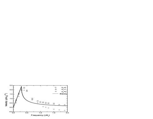
Figure 3: DW propagation velocity $\upsilon$ as a function of CPMF frequency $\omega$ for $\alpha=0.1$, $h_{0}=3$ and $K_{1}=8$. Symbols are results of numerical simulations for $K_{2}=0$ (squares), $1$ (triangles), and $3$ (hexagons), respectively. Solid curve corresponds to the theoretical result for $K_{2}=0$.

In conclusion, CPMF at GHz frequency is an efficient control parameter for DW motion. Two propagation modes are identified. Under a low frequency ($\omega<\omega_{c}$), a DW propagates like a rigid body at a constant velocity that increases linearly with the CPMF frequency. At a high frequency ($\omega>\omega_{c}$), DW propagation speed is oscillatory whose time-averaged value decreases with the frequency. For a uniaxial wire, a DW under a CPMF can be mapped to the DW under STT due to uniform spin-polarized current. In the map, the CPMF frequency plays the role of the spin polarized current.

This work is supported by Hong Kong UGC/CERG grants (#603007, 603508 and SBI07/08.SC09). We thank J. Lu for helping numerical simulations.

References

- (1) N.L. Schryer and L.R. Walker, J. Appl. Phys. 45, 5406 (1974).
- (2) D. Atkinson, D.A. Allwood, G. Xiong, M.D. Cooke, C. Faulkner, and R.P. Cowburn, Nature Mater. 2, 85 (2003).
- (3) G.S.D. Beach, C. Knutson, C. Nistor, M. Tsoi, and J.L. Erskine, Phys. Rev. Lett. 97, 057203 (2006).
- (4) X.R. Wang, P. Yan, J. Lu and C. He, Annals of Physics 324, 1815 (2009); X.R. Wang, P. Yan, J. Lu, Europhys. Lett. 86, 67001 (2009).
- (5) J. Slonczewski, J. Magn. Magn. Mater. 159, L1 (1996); L. Berger, Phys. Rev. B 54, 9353 (1996).
- (6) S. Zhang, P. M. Levy, and A. Fert, Phys. Rev. Lett. 88, 236601 (2002).
- (7) S. Zhang and Z. Li, Phys. Rev. Lett. 93, 127204 (2004).
- (8) J. Grollier, P. Boulenc, V. Cros, A. Hamzic, A. Vaures, and A. Fert, Appl. Phys. Lett. 83, 509 (2003).
- (9) M. Hayashi, L. Thomas, Y.B. Bazaliy, C. Rettner, R. Moriya, X. Jiang, and S.S.P. Parkin, Phys. Rev. Lett. 96, 197207 (2006); M. Hayashi, L. Thomas, C. Rettner, R. Moriya, Y.B. Bazaliy, and S.S.P. Parkin, Phys. Rev. Lett. 98, 037204 (2007).
- (10) S.S.P. Parkin, M. Hayashi, L. Thomas, Science 320, 190 (2008).
- (11) Z. Li, S. Zhang, Z. Diao, Y. Ding, X. Tang, D.M. Apalkov, Z. Yang, K. Kawabata, and Y. Huai, Phys. Rev. Lett. 100, 246602 (2008).
- (12) A.V. Khvalkovskiy, K.A. Zvezdin, Ya.V. Gorbunov, V. Cros, J. Grollier, A. Fert, and A.K. Zvezdin, Phys. Rev. Lett. 102, 067206 (2009).
- (13) Z.Z. Sun, and X.R. Wang, Phys. Rev. B 74, 132401 (2006).
- (14) T. Moriyama, R. Cao, J.Q. Xiao, J. Lu, X.R. Wang, Q. Wen, and H.W. Zhang, Appl. Phys. Lett. 90, 152503 (2007); J. Appl. Phys. 103, 07A906 (2008).
- (15) Although various torques on individual spins are the ultimate microscopic ”forces” for DW dynamics. Energy may be a better quantity to understand the origin of DW propagation. For detail, see Reference 4.
- (16) T. L. Gilbert, IEEE Trans. Magn. 40, 3443 (2004).
- (17) Z.Z. Sun and X.R. Wang, Phys. Rev. Lett. 97, 077205 (2006); X.R. Wang and Z.Z. Sun, ibid 98, 077201 (2007).
- (18) Vladimir L. Sobolev, Huei Li Huang, and Shoan Chung Chen, J. Appl. Phys. 75, 5797 (1994).
- (19) G. Tatara and H. Kohno, Phys. Rev. Lett. 92, 086601 (2004).
- (20) Z. Li and S. Zhang, Phys. Rev. Lett. 92, 207203 (2004).
- (21) S.E. Barnes and S. Maekawa, Phys. Rev. Lett. 98, 246601 (2007).
- (22) Shengyuan A. Yang, Geoffrey S.D. Beach, Carl Knutson, Di Xiao, Qian Niu, Maxim Tsoi, and James L. Erskine, Phys. Rev. Lett. 102, 067201 (2009).