Learning Out of Leaders

Abstract

This paper investigates the estimation problem in a regression-type model. To be able to deal with potential high dimensions, we provide a procedure called LOL, for Learning Out of Leaders with no optimization step. LOL is an auto-driven algorithm with two thresholding steps. A first adaptive thresholding helps to select leaders among the initial regressors in order to obtain a first reduction of dimensionality. Then a second thresholding is performed on the linear regression upon the leaders. The consistency of the procedure is investigated. Exponential bounds are obtained, leading to minimax and adaptive results for a wide class of sparse parameters, with (quasi) no restriction on the number $p$ of possible regressors. An extensive computational experiment is conducted to emphasize the practical good performances of LOL.

1 Introduction

The general linear model is considered here, with a particular focus on cases where the number $p$ of regressors is large compared to the number $n$ of observations (although there is no such restrictions). These kinds of models have today a lot of practical applications in many areas of science and engineering including collaborative filtering, machine learning, control, remote sensing, and computer vision just to name a few of them. Examples in statistical signal processing and nonparametric estimation include the recovery of a continuous-time curve or a surface from a finite number of noisy samples. Other interesting fields of application are radiology and biomedical imaging when fewer measurements about an image are available compared to the unknown number of pixels collected. In biostatistics, high dimensional problems frequently arise specially in genomic when gene expression are studied given a huge number of initial genes compared to a relatively low number of observations.

A considerable amount of work has been produced in this domain in the last years, which has been a large source of inspiration for this paper: algorithms coming from the learning framework Barron et al. (2008), Binev et al. (2005), Binev et al. (2007a), Binev et al. (2007b)), as well as the extraordinary explosive domain of $\ell_{1}$ penalties, among many others Tibshirani (1996), Candes and Tao (2007), Bickel et al. (2008), Bunea et al. (2007a), Bunea et al. (2007b), Fan and Lv (2008) and Candès and Plan (2009). See also Lounici (2008) and Alquier and Hebiri (2009).

The essential motivation of this work is to provide one of the simplest procedures that achieves, in the same time, good performances. LOL algorithm (for Learning Out of Leaders) consists in a two steps thresholding procedure. As there is no optimization step, it is important to address the following question: what are the domains where the procedure is competitive compared to more sophisticated algorithms, especially to algorithms performing one or two steps $\ell_{1}$ minimization ? One of our aim here is not only to delimit where LOL is competitive but also to point out where the simplicity of LOL induces a slight lack of efficiency from both a theoretical point of view as from a practical aspect.

Let us start by introducing the ideas of the emergence of LOL algorithm. This simple procedure can be viewed as an ’explanation’ or as a ’cartoon’ of $\ell_{1}$ minimizations. It is well known that when the regressors are normalized and orthogonal, $\ell_{1}$ minimization corresponds to soft thresholding which itself is close to hard thresholding. Hence, it is quite natural to expect that thresholding should perform well, at least in cases not too far from these orthonormal conditions. It corresponds, as specified below, to small coherence conditions. A tricky problem occurs when the regressors are not orthonormal or when the number of regressors is large. Then, the minimum least squares estimator has a non unique solution and the solutions are very unstable. This is the heart and the main difficulty for the $\ell_{1}$ minimizers or more generally for all methods based on sparsity assumptions. In order to be solved, the problem requires essentially -as will be discussed extensively in the sequel- two types of conditions: sparsity of the solution and isometry properties for the matrix of regressors. This is often the part where the algorithms computation cost shows up. Obviously a simple thresholding would not fit, but the above mentioned conditions can ensure that it is at least possible to select some regressors and exclude some others. LOL algorithm solves the difficult problem of the choice of the regressors in a quite crude way by adaptively selecting $N$ regressors which are the most correlated to the target: this defines the first step thresholding of LOL, determining the $N$ leaders. The number $N$ is chosen using a fine tuning parameter depending on the coherence. It has to be emphasized that the choice is auto driven in the algorithm. In a second thresholding step, LOL regresses on the leaders, then thresholds the estimated coefficients taking into account the noise of the model.

The properties of LOL are here investigated specifically for the prediction problem. More precisely, it is established in this paper that LOL has a prediction error which is going to zero in probability with exponential rates. These types of results are often called Bahadur type efficiency. Although Bahadur efficiency of test and estimation procedures goes back to the sixties (see Bahadur (1960)), it has seen recently a revival in learning theory, where the rates of convergence (preferably exponential) of the procedures are investigated and compared to optimality. It is also related to a common concept in learning theory: The Probably Approximately Correct (PAC) learning paradigm introduced in Valiant (1984).

Of course, because of the straightforwardness of the method, some loss of efficiency is expected compared to more elaborate and costly procedures. But even with a loss, the limitations of the procedure can bring an interesting information on the $\ell_{1}$ minimizers themselves. From both theoretical and practical point of view, with small coherence, LOL procedure appears to be as powerful as the best known procedures. The exponential rates of convergence match for instance the lower bounds obtained in Raskutti et al. (2009). This result is obtained under minimal conditions on the number $p$ of potential regressors. Also even with a loss in the rate, a positive aspect is that the practitioner is informed of the possible instability of the method since the coherence can be computed using the observations before any calculation. This is notably not the case for usual conditions such as RIP or even more abstract ones which are impossible to verify in practice. An intensive calculation program is performed to show the advantages and limitations of LOL procedure in several practical aspects. The case where the regressors are forming a random design matrix with i.i.d. entries is investigated in Section 6. Different laws of the inputs are studied (Gaussian, Uniform, Bernoulli or Student laws) inducing a specific coherence for the design matrix. Several interesting features are also discussed in this section. Dependent inputs are simulated and an application with real data is also discussed. The impact of the sparsity and the undetermination of the regression on the performances of LOL are studied. A comparison with two others two-step procedures namely Fan and Lv (2008) and Candès and Plan (2009) is also performed. The most interesting conclusion being that the practical results are even better and more comforting than the theoretical ones in the sense that LOL shows good performances, even when the coherence is pretty high.

To summarize this presentation and answer to the question ”In what type of situations should a practitioner prefer to use LOL rather than other available methods?”, our results and our work prove that when the number of regressors $p$ is very large, and when the computational aspects of optimization procedures become difficult as well as the theoretical results uncertain, LOL should be preferred by a practitioner after ensuring (and this is done by a simple calculation) that the coherence is not too high. On the other hand when the coherence is very high, one should probably be suspicious enough regarding any method…

The paper is organized as follows. In Section 2, the general model and the notations are presented. In Section 3, LOL is detailed as other procedures with a $\ell_{1}$ optimization step; Comparisons with other procedures are later discussed in Section 5. In Section 4, after stating the hypotheses needed on the model, theoretical results are established. The practical performances of LOL are investigated in Section 6 and the proofs are detailed in Section 7.

2 Model and coherence

2.1 General model

In this paper, we observe a pair $(Y,\Phi)\;\in\mathbb{R}^{n}\times\mathbb{R}^{n\times p}$ where $\Phi$ is the design matrix and $Y$ a vector of response variables. These two quantities are linked by the standard linear model

$$Y =\Phi\alpha+u+\varepsilon$$ (1)

where the parameter $\alpha\in\mathbb{R}^{p}$ is the unknown vector to be estimated and

• the vector $\varepsilon=(\varepsilon_{1},\ldots,\varepsilon_{n})^{t}$ is a (non observed) vector of random errors. It is assumed to be independent Gaussian variables $N(0,\sigma^{2})$ but essentially comparable results can be obtained in the case of zero mean subgaussian errors (see the remark before Lemma 3).

• the vector $u=(u_{1},\ldots,u_{n})^{t}$ is a non observed vector of (possibly) random errors. Its amplitude is assumed to be small. The differences between the two previously described ”errors” lies in the fact that the $\varepsilon_{i}$’s are centered but unbounded and independent, while the $u_{i}$’s are only bounded. The necessity of introducing these two types of errors becomes clear in the functional regression example.

• $\Phi$ is a $n\times p$ known matrix. This paper focuses on the interesting case where $p\gg n$ but it is not necessary. We assume that $\Phi$ has normalized columns (or normalized them) in the following sense:

  $$\frac{1}{n}\sum_{i=1}^{n}\Phi_{i\ell}^{2}=1,\quad\forall\;\ell=1\ldots,p.$$ (2)

2.2 Examples

An example of such a model occurs when the matrix $\Phi$ is a random matrix composed of $n$ independent and mainly identically distributed random vectors of size $p$. The simulation study given in Section 6 details the important role played by the distribution of these random vectors.

A second application is the learning (also called functional regression) model

$$Y_{i}=f(X_{i})+\varepsilon_{i},\;i=1\ldots n$$ (3)

where $f$ is the parameter of interest. This model is classically related to the previous one using a dictionary $\mathcal{D}=\{g_{l},\;l\leq p\}$ of size $p$, $\Phi$ becoming then the matrix with general term $\Phi_{i\ell}=g_{\ell}(X_{i})$. Assuming that $f$ can be reasonably well approximated using the elements of the dictionary means that $f$ can be written as $f=\sum_{g\in\mathcal{D}}\alpha_{g}g+h$ where $h$ is hopefully small. It becomes clear here that $u_{i}=h(X_{i})$. This case has been investigated in more details in Kerkyacharian et al. ) using an earlier and less elaborated version of LOL.

2.3 Coherence

In the sequel, the following notations are used. Let $m$ be an integer and $q>0$, for any $x\in\mathbb{R}^{m}$,

$$\|x\|_{l^{q}(m)}\,:=\,\left(\sum_{k=1}^{m}|x_{k}|^{q}\right)^{1/q}$$

denotes the $l^{q}(\mathbb{R}^{m})-$norm (or quasi norm) and, for any $x\in\mathbb{R}^{n}$,

$$\|x\|_{n}^{2}\,:=\,\frac{1}{n}\|x\|_{{l}_{2}(n)}^{2}$$

denotes the quadratic empirical norm. We define the following $p\times p$ Gram matrix as

$$M:=\frac{1}{n}\Phi^{t}\Phi.$$

The quantity

$$\tau_{n}=\sup_{\ell\not=m}|M_{\ell m}|=\sup_{\ell\not=m}|\frac{1}{n}\sum_{i=1}^{n}\Phi_{i\ell}\Phi_{im}|$$

is called the coherence of the matrix $M$. Observe that $\tau_{n}$ is a quantity directly computable from the data. It is also a crucial quantity because it induces a bound on the size of the invertible matrices built with the columns of $M$. More precisely, fix $0<\nu<1$ and let $\mathcal{I}$ be a subset of indices of $\{1,\ldots,p\}$ with cardinality $m$. Denote $\Phi_{|\mathcal{I}}$ the matrix restricted to the columns of $\Phi$ whose indices belong to $\mathcal{I}$. If $2\tau_{n}\leq\nu$, the associated Gram matrix

$$M(\mathcal{I}):=\frac{1}{n}\Phi_{|\mathcal{I}}^{t}\Phi_{|\mathcal{I}}$$

is almost diagonal as soon as $m$ is smaller than $N:=\lfloor\nu/\tau_{n}\rfloor$ (where $\lfloor\nu/\tau_{n}\rfloor$ denotes the integer part of $\nu/\tau_{n}$) in the sense that it satisfies the following so called Restricted Isometry Property (RIP)

$$\forall x\in\mathbb{R}^{m},\;\ \|x\|_{{l}_{2}(m)}^{2}(1-\nu)\leq x^{t}{\mathcal{M}}(\mathcal{I})x\leq\|x\|_{{l}_{2}(m)}^{2}(1+\nu)\;.$$ (4)

This proves in particular that the matrix $M(\mathcal{I})$ is invertible. The proof of (4) is simple and can be found together with a discussion on the relations between RIP Property and conditions on the coherence, for instance in Blanchard et al. (2009). The RIP Property (4) can be rewritten as follows. The following lemma is a key ingredient of our proofs.

Lemma 1

Let $\mathcal{I}$ be a subset of $\{1,\ldots,p\}$ satisfying $\#(\mathcal{I})\leq N$. For any $x\;\in\mathbb{R}^{\#(\mathcal{I})}$, we get

$$(1-\nu)\,\|x\|_{l^{2}(\#(\mathcal{I}))}^{2}\leq\|\sum_{\ell\in\mathcal{I}}x_{\ell}\;\Phi_{\bullet\ell}\;\|_{n}^{2}\leq(1+\nu)\,\|x\|_{l^{2}(\#(\mathcal{I}))}^{2}.$$

3 Estimation procedures

In this section, the estimation of the unknown parameter $\alpha$ using LOL is described first. Next, a short review on the procedures directly connected to LOL is proposed.

Once for all, the constant $\nu$ is fixed. This constant is obviously related to the precision of LOL main procedure: the default value here considered is $\nu=0.5$.

3.1 LOL Procedure

As inputs, LOL algorithm requires 4 pieces of information:

• The observed variable $Y$ and the regression variables $\Phi=(\Phi_{\bullet 1},\ldots\Phi_{\bullet p})$.

• The tuning parameters $\lambda_{n}(1)$ and $\lambda_{n}(2)$ giving the level of the thresholds.

Observe that the algorithm is adaptive in the sense that no information on the sparsity of the sequence $\alpha$ is necessary. An upper bound for the cardinal of the set of leaders is first computed: $N\leftarrow\lfloor\nu/\tau_{n}\rfloor$. Thereafter, LOL performs two major steps:

• Find the leaders by thresholding the ”correlation” between $Y$ and the $\Phi_{\bullet\ell}$’s at level $\lambda_{n}(1)$. ${\mathcal{B}}$ denotes the set of indices of the selected leaders. The size of this set is bounded with $N$ by retaining only (when necessary) the indices with maximal correlations.

• Regress $Y$ on the leaders $\Phi_{|{\mathcal{B}}}=(\Phi_{\bullet\ell})_{\ell\in{\mathcal{B}}}$ and threshold the result at level $\lambda_{n}(2)$.

The following pseudocode gives details of the procedure. Note that there is no step of optimization and no iteration procedure.

LOL$(\Phi,Y,\lambda_{n}(1),\lambda_{n}(2))$

Input: observed data $Y$, regression variables $\Phi$, tuning parameters $\lambda_{n}(1),\lambda_{n}(2)$

Output: estimated parameters $\widehat{\alpha^{*}}$, and predicted value $\widehat{Y}$

STEP 0	{Initialize}
$\nu=0.5$
$\tau_{n}\leftarrow n^{-1}\,\max_{\ell\not=m}|\sum_{i=1}^{n}\Phi_{i\ell}\Phi_{im}|$	{Compute the coherence}
$N\leftarrow\lfloor\frac{\nu}{\tau_{n}}\rfloor$	{Compute the upper bound
	for the cardinal of the leaders set}
STEP 1	{Find the leaders}
For $\ell=1:p$
$\widetilde{\alpha_{\ell}}\leftarrow\frac{1}{n}\,\sum_{i=1}^{n}\Phi_{i\ell}Y_{i}$	{Compute the ’correlations’
	between the observations and the regressors }
$\widetilde{\alpha_{\ell}}^{*}\leftarrow\widetilde{\alpha_{\ell}}{\mathbb{I}}\{|\widetilde{\alpha_{\ell}}|\geq\lambda_{n}(1)\}$	{Threshold }
End(for)
${\mathcal{B}}\leftarrow\{\ell,\widetilde{\alpha_{\ell}}^{*}\not=0\}$	{Determine the leaders}
If $\#{\mathcal{B}}>N$
indices $\leftarrow$ sort$(|\widetilde{\alpha}|)$	{Sort the ’correlations’ of the candidates}
${\mathcal{B}}\leftarrow$ indices$[1:N]$	{Take the indices associated to the $N-$th largest}
End(if)
STEP 2	{Regress on the leaders}
$\widehat{\alpha}_{|{\mathcal{B}}}\leftarrow(^{t}\Phi_{|{\mathcal{B}}}\Phi_{|{\mathcal{B}}})^{-1}\Phi_{|{\mathcal{B}}}Y$	{Least square estimators}
$\widehat{\alpha}^{*}_{|{\mathcal{B}}}\leftarrow\widehat{\alpha}_{|{\mathcal{B}}}\,{\mathbb{I}}\{|\widehat{\alpha}_{|{\mathcal{B}}}|\geq\lambda_{n}(2)\}$	{Threshold}
$\widehat{\alpha}^{*}_{|{\mathcal{B}}^{c}}\leftarrow 0$
$\widehat{Y}\leftarrow\Phi\,\widehat{\alpha}^{*}$	{Find the predicted value}

3.2 Several inspirations

Although it is impossible to be exhaustive in such a productive domain, some of the works directly in relation to our construction are hereafter mentioned. We apologize in advance for all the works that are not mentioned but still remain in connection. For a comprehensive overview, we refer to Fan and Lv (2010).

Several authors propose procedures to solve the selection problem or the estimation problem in cases where the vector $\alpha$ has only a small number of non zero components, and (often) when the design matrix $\Phi$ is composed of i.i.d. random vectors: see among many others Tibshirani (1996), Candes and Tao (2007), Bickel et al. (2008), Bunea et al. (2007a) and Bunea et al. (2007b).

A focus is particulary made here on the 2-steps procedures which are also commonly used, and apparently for a long time, since in 1959 such a procedure is already discussed (see Satterthwaite (1959)). In Candes and Tao (2007) and Candès and Plan (2009), the leaders are selected with respectively the Dantzig procedure and the Lasso procedure. Then, the estimated coefficients are computed using a linear regression on the leaders. Using an intensive simulation program, Fan and Lv (2008) show that it could be unfavorable to use the procedures Lasso or Dantzig before the reduction of the dimension. They also provide a search among leaders called Sure Independence Screening (SIS) procedure. This procedure is similar to the one discussed in this paper: The leaders are the $N=\lfloor\gamma_{n}n\rfloor$ columns of $\Phi$ with largest correlations to the target variable $Y$ ($\gamma_{n}$ is a tuning sequence tending to zero). This step is followed with a subsequent estimation procedure using Dantzig or Lasso. All these methods show a higher complexity compared to LOL.

LOL procedure can also be connected to the family of Orthogonal Matching Pursuit algorithms as well as in general to the Greedy Algorithms. For this interesting literature, we refer among others to Needell and Tropp (2009), Tropp and Gilbert (2007), Barron et al. (2008). The main advantage of LOL compared to this kind of algorithms is that there is no iterative search of the leaders. All the leaders are selected in one shot and the procedure stops just after the second step. Moreover, convergence results are almost as good as those procedures in many situations.

4 Main theoretical results

This section states the theoretical results of LOL procedure. The measures of performances used in the theorems are first presented, then the assumptions on the set of parameters $\alpha$ are given.

4.1 Loss fonction

Let us define the following loss function to measure the difference between the true value $\alpha\;\in\mathbb{R}^{p}$ and the result $\hat{\alpha}^{*}$ computed by LOL. Denote $\Phi_{i\bullet}$ the $i-$th line of the matrix $\Phi$ and recall that the $i-$th observation is given by the model:

$$Y_{i}=\Phi_{i\bullet}\alpha+u_{i}+\varepsilon_{i}.$$

The predicted $i-$th observation is $\widehat{Y_{i}}=\Phi_{i\bullet}\hat{\alpha}^{*}$. The criterium of performance is defined by the empirical quadratic distance between the predicted variables and their expected values.

$$d(\hat{\alpha}^{*},\alpha)^{2}=\frac{1}{n}\sum_{i=1}^{n}\left(\widehat{Y_{i}}-{\mathbb{E}}Y_{i}\right)^{2}=\frac{1}{n}\sum_{i=1}^{n}\left(\sum_{\ell=1}^{p}(\hat{\alpha}_{\ell}^{*}-\alpha_{\ell})\Phi_{i\ell}+u_{i}\right)^{2}$$

which can be rewritten using the empirical norm

$$d(\hat{\alpha}^{*},\alpha):=\|\sum_{\ell=1}^{p}(\hat{\alpha}_{\ell}^{*}-\alpha_{\ell})\Phi_{\bullet\ell}+u_{\bullet}\|_{n}.$$

Observe that the considered loss is the usual error of prediction

$$d(\hat{\alpha}^{*},\alpha)=\|\Phi(\hat{\alpha}^{*}-\alpha)\|_{n}$$

when the ’errors’ $u_{i}$’s are all zero.

4.2 Bahadur-type efficiency

Our measure of performance is issued from the Bahadur efficiency of test and estimation procedures and is defined for any tolerance $\eta>0$ as

$${AC}_{n}(LOL,\eta,\alpha)=P\left(d(\hat{\alpha}^{*},\alpha)>\eta\right).$$ (5)

This quantity measures a confidence that the estimator is accurate to the tolerance $\eta$ if the true point is $\alpha$. We also define and consider uniform confidence over a class $\Theta$ :

$${AC}_{n}(LOL,\eta,\Theta)=\sup_{\alpha\in\Theta}P\left(d(\hat{\alpha}^{*},\alpha)>\eta\right).$$ (6)

This quantity has been studied for instance in DeVore et al. (2006) in the learning framework. In most examples, it is proved that there exist a phase transition and a critical value $\eta_{n}$ depending on $n$ and $\Theta$ such that ${AC}_{n}(\hat{f},\eta,\Theta)$ decreases exponentially for any $\eta>\eta_{n}$. More precisely, in terms of lower bound -but similar bounds are also valid in terms of upper bounds-, it is proved in DeVore et al. (2006) that

$$\inf_{\hat{f}}{AC}_{n}(\hat{f},\eta,\Theta)\geq C\sqrt{\bar{N}(\Theta,\eta)}e^{-cn\eta^{2}},$$ (7)

where $\bar{N}(\Theta,\eta)$ is the tight entropy analogue of the Sobolev covering numbers. On this expression, $\eta_{n}$ appears quite convincingly as a turning point after which the exponential term dominates the entropy term. Observe that the critical value $\eta_{n}$ is essential since it yields bounds for $\sup_{\alpha\in\Theta}E_{\alpha}d(\hat{\alpha}^{*},\alpha)$ which is another (more standard) measure of performance of the procedure. The results in DeVore et al. (2006) are obtained in the learning framework; however identical bounds can easily be expected in the setting (1) of this paper, as results obtained in Raskutti et al. (2009). This is discussed in more details in the sequel since similar bounds are obtained for LOL with sparsity constraints defined below.

4.3 Performances of the procedure LOL. $l_{q}$ ball constraints

In this part, we consider the following sparsity constraint

$$\mbox{for }q\in(0,1],\quad B_{q}(M):=\{\alpha\in\mathbb{R}^{p},\;\|\alpha\|_{l^{q}(p)}\leq M\}$$

or

$$\mbox{for }q=0,\quad B_{0}(S,M):=\{\alpha\in\mathbb{R}^{p},\;\sum_{j=1}^{p}I\{|\alpha_{j}\not=0\}\leq S,\;\|\alpha\|_{l^{1}(p)}\leq M\}.$$

Theorem 1

Let $M>0$ and fix $\nu$ in $]0,1[$. Assume that there exists a positive constant $c^{\prime}$ such that $p\leq\exp(c^{\prime}n)$. Suppose there exist positive constants $c,c_{0}$ such that

$$\tau_{n}\leq c\sqrt{\frac{\log p}{n}}\quad\mbox{ and }\quad\sup_{i=1,\ldots,n}|u_{i}|\leq c_{0}\;\sqrt{\frac{1}{n}}.$$ (8)

Let us choose the thresholds $\lambda_{n}(1)$ and $\lambda_{n}(2)$ such that

$$\lambda_{n}(2)=T_{3}\sqrt{\frac{\log{p}}{n}}\quad\mbox{ and }\quad\lambda_{n}(1)=T_{4}\sqrt{\frac{\log{p}}{n}}$$

for $T_{4}\geq T_{1}\vee T_{2}\,c\vee T_{3}>0$ where

$$T_{1}=\left(64\sigma\vee 1\vee\frac{2}{(1-\nu)\sigma}\right)\mbox{ and }T_{2}=\left(6M\vee\frac{(4M+3c_{0})}{12\sigma}\right).$$

Then, there exist positive constants $D$ and $\gamma$ depending on $\nu,c,c^{\prime},c_{0},T_{3},T_{4}$ such that

$$\sup_{\alpha\in\;B_{q}(M)}{\mathbb{P}}\left(d(\hat{\alpha}^{*},\alpha)>\eta\right)\leq\left\{\begin{array}[]{lll}4e^{-\gamma n\eta^{2}}&\mbox{ for }&\eta^{2}\geq D\;\left(\frac{\log p}{n}\right)^{1-q/2}\\ &&\\ 1&\mbox{ for }&\eta^{2}\leq D\;\left(\frac{\log p}{n}\right)^{1-q/2}\end{array}\right.$$

and

$$\sup_{\alpha\in\;B_{0}(S,M)}{\mathbb{P}}\left(d(\hat{\alpha}^{*},\alpha)>\eta\right)\leq\left\{\begin{array}[]{lll}4e^{-\gamma n\eta^{2}}&\mbox{ for }&\eta^{2}\geq D\;\frac{S\,{\log p}}{n}\\ &&\\ 1&\mbox{ for }&\eta^{2}\leq D\;\frac{S\,\log{p}}{n}\end{array}\right.$$

for any $S<\nu/\tau_{n}$.

We immediately deduce the following bound for the usual expected error

Corollary 1

For $r\geq 1$ arbitrary, under the same assumptions as in Theorem 1, we have

$$\sup_{B_{q}(M)}{\mathbb{E}}d(\hat{\alpha}^{*},\alpha)^{r}\leq D^{\prime}\left(\frac{\log p}{n}\right)^{(1-q/2)r/2}$$

for some positive constant $D^{\prime}$ depending on $\nu,c,c^{\prime},c_{0},T_{3},T_{4}$, as well as

$$\sup_{B_{0}(S,M)}{\mathbb{E}}d(\hat{\alpha}^{*},\alpha)^{r}\leq D^{\prime}\left(\frac{S\log p}{n}\right)^{r/2}$$

for any $S<\nu/\tau_{n}$.

4.4 Performances of LOL procedure. MaxiSet point of view

In this section we develop a slightly different point of view issued from the maxiset theory (see for instance Kerkyacharian and Picard (2000)). More precisely our aim is to evaluate the quality of our algorithm when the coherence and thresholding tuning constants are given (fixed). Especially, it means that we do not assume in this part that the coherence satisfies $\tau_{n}\leq O(\sqrt{\log{p}/n})$. For that, we consider a set $V(S,M)$ of parameters $\alpha$ depending on these constants $M,S>0$ and prove that the right exponential decreasing of the confidence is achieved on this set. The phase transition $\eta_{n}$ is depending on the tuning constants and of the coherence in the following way

$$\eta_{n}^{2}=O(\frac{S\log p}{n}\vee S\tau_{n}^{2}).$$

Observe that we do not prove that the set $V(S,M)$ is exactly the maxiset of the method (considered in terms of $\eta_{n}$) since we do not not prove that it is the largest set with the phase transition $\eta_{n}$. However the following theorem reflects quite extensively the theoretical behavior of LOL, even in case of deterioration due to a high coherence or a bad choice of the thresholds. Notice also that Theorem 1 is a quite easy consequence of Theorem 2.

Let us now define the set $V(S,M)$ by the following sparsity constraints. There exist $S\leq\lfloor\nu/\tau_{n}\rfloor$ and constants ${M},\;c_{0},\;c_{1},\,c_{2}$, such that the vector $\alpha\in\mathbb{R}^{p}$ satisfies the following conditions

$$\|\alpha\|_{l^{1}(p)}\leq{M},$$ (9)

$$\#\left\{\ell\in\{1,\ldots,p\},\;|\alpha_{\ell}|\geq\lambda_{n}(2)/2\right\}\;\leq{S}$$ (10)

$$\sum_{(\ell)>N}|\alpha_{(\ell)}|\leq c_{1}\;\left(\frac{S\log p}{n\tau_{n}}\right)^{1/2}$$ (11)

$$\sum_{\ell=1}^{p}|\alpha_{\ell}|^{2}\;I\{|\alpha_{\ell}|\leq 2\lambda_{n}(1)\}\leq c_{2}^{2}\;\frac{S\log p}{n}$$ (12)

Recall that $(\alpha_{(\ell\,)})$ is the ordered sequence (for the modulus) $|\alpha_{(1)}|\geq|\alpha_{(2)}|\geq\ldots|\alpha_{(p)}|$. For $S,M>0$, $V(S,M)$ denotes the class of models of type (1) satisfying the sparsity conditions (9), (10), (11), (12). Note that we emphasize in the notation of the set $V(S,M)$ the constants $S$ and $M$, while the set is depending on other additional constants, since these two constants play a crucial role.

Theorem 2

Let $S,M>0$ and fix $\nu$ in $]0,1[$. The thresholds $\lambda_{n}(1)$ and $\lambda_{n}(2)$ are chosen such that

$$\lambda_{n}(1)\geq\left(T_{1}\left(\frac{\log{p}}{n}\right)^{1/2}\vee T_{2}\,\tau_{n}\right)\quad\mbox{ and }\quad\lambda_{n}(2)\leq\lambda_{n}(1)$$

$$T_{1}=\left(64\sigma\vee 1\vee\frac{2}{(1-\nu)\sigma}\right)\mbox{ and }T_{2}=\left(6M\vee\frac{(4M+3c_{0})}{12\sigma}\right).$$

Then, if in addition we have

$$\sup_{i=1,\ldots,n}|u_{i}|\leq c_{0}\;\left(\frac{S}{n}\right)^{1/2}$$ (13)

there exist positive constants $D$ and $\gamma$ depending on $\nu,\sigma^{2},M,c_{0},c_{1},c_{2}$, such that

$$\sup_{\alpha\in\;V(S,M)}{\mathbb{P}}\left(d(\hat{\alpha}^{*},\alpha)>\eta\right)\leq\left\{\begin{array}[]{lll}4e^{-\gamma n\eta^{2}}&\mbox{ for }&\eta^{2}\geq D\;\left(\frac{S\log p}{n}\vee\ S\tau_{n}^{2}\right),\\ &&\\ 1&\mbox{ for }&\eta^{2}\leq D\;\left(\frac{S\log p}{n}\vee S\tau_{n}^{2}\right)\end{array}\right.$$ (14)

For a sake of completeness, the constants $D$ and $\gamma$ are precisely given at the end of the proof of Theorem 2. However, it is obvious that the constants provided here are not optimal: for instance in the proof, in order to avoid unnecessary technicalities, most of the events are divided as if they had an equal importance, leading to constants which are each time divided by 2. Obviously there is some place for improvement at any of these stages.

An elementary consequence of Theorem 2 is the following corollary which details the behavior of the expectation of $d(\hat{\alpha}^{*},\alpha)$. Notice also that we did not give here explicit oracle inequalities, which however could be derived from the proof of Theorem 2.

Corollary 2

For $r\geq 1$ arbitrary, under the same assumptions as in Theorem 2, we get

$$\sup_{V(S,M)}{\mathbb{E}}d(\hat{\alpha}^{*},\alpha)^{r}\leq D^{\prime}\left(\frac{S\log{p}}{n}\vee S\tau_{n}^{2}\right)^{r/2}$$

for some positive constant $D^{\prime}$ depending on $\nu,\sigma^{2},M,c_{0},c_{1},c_{2}$ and $r$.

5 Remarks and Comparisons

5.1 Results under $l_{q}$ constraints

It is important to discuss the relations of the results in Theorem 1 with Raskutti et al. (2009) which provides minimax bounds in a setting close to ours. Their results basically concern exponential inequalities (as ours) but they are only interested in the case $\eta=\eta_{n}$ for which they prove upper and lower bounds. If we compare our results to theirs, we find that LOL is exactly minimax for any $q$ in $(0,1]$, with even a better precision since we prove the exponential inequality for any $\eta$. In the case $q=0$, we have a slight logarithmic loss. Notice that we also need a bound on $\|\alpha\|_{l^{1}(p)}$. We do not know if this is due to our proof or specific to the method.

5.2 Ultra high dimensions

One main advantage of LOL is that it is really designed for very large dimensions. As seen in the results of Theorem 1 and Theorem 2, no limitation on $p$ is required except $p\leq\exp(cn)$ (in fact this is only needed in Theorem 1). Notice that, if this condition is not satisfied, not any algorithm is convergent as proved by the lower bound of Raskutti et al. (2009). Moreover, the fact that the algorithm has no optimization step is a serious advantage when $p$ becomes large.

5.3 Adaptation

Our theoretical results are provided under conditions on the tuning quantities $\lambda_{n}(1)$ and $\lambda_{n}(2)$. The default values issued from the theoretical results are the following

$$\lambda_{n}^{*}(1)=\lambda_{n}^{*}(2)=\left(T_{1}\sqrt{\frac{\log{p}}{n}}\vee T_{2}\,\tau_{n}\right).$$

It is a consequence of Theorem 1 that LOL associated with $\lambda_{n}^{*}(1)$ and $\lambda_{n}^{*}(2)$ is adaptive over all the sets $B_{q}(M)$ and $B_{0}(S,M)$, with respect to the parameters $q$ and $S$. These default values behave also reasonably well in practice. However, they require a fine tuning of the constants $T_{1}$ and $T_{2}$ which is proposed in a slightly more subtle way in the simulation part (see Section 6).

5.4 Coherence condition

As can be seen in Theorem 1, LOL is minimax under a condition on the coherence of the type $\tau_{n}\leq c\sqrt{\log{p}/n}$. This condition is verified with overwhelming probability for instance when the entries of the matrix $\Phi$ are independent and identically random variables with a sub-gaussian common distribution. In Section 6, we precisely investigate the behavior of LOL when this hypothesis is disturbed. This bound is generally stronger as a condition compared to other ones given in the literature such as the RIP condition, or weaker ones. However, as explained in the sequel, these other conditions are often impossible to verify on the data. We consider as a benefit that the procedure is giving with $\tau_{n}$ an indication of a potential misbehavior. Besides, Theorem 2 details the behavior of the algorithm when this condition is not verified.

5.5 Comparison with some existing algorithms

As mentioned in the previous section, LOL finds its inspiration in the learning framework, especially in Barron et al. (2008), Binev et al. (2005), Binev et al. (2007a),Binev et al. (2007b). In all these papers, consistency results are obtained under fewer assumptions but with no exponential bounds and a higher cost in implementation. Again in the learning context, Temlyakov (2008) provides optimal critical value $\eta_{n}$ as well as exponential bounds with fewer assumptions since there is no coherence restriction. However, the procedure is very difficult to implement for large values of $p$ and $n$ ($N$-$P$ hard).

In Fan and Lv (2008), it is assumed that there exists $\kappa>0$ such that

$$\min_{\ell\in{\mathcal{I}}^{*}}|\alpha_{\ell}|\geq O(n^{-\kappa})$$

where ${\mathcal{I}}^{*}=\{\ell,\alpha_{\ell}\not=0\}$. The model under consideration is ultra high dimensioned: $p\leq\exp(cn^{\xi})$ for $c,\xi>0$ with the restriction $\xi<1-2\kappa<1$. The procedure SIS-D (SIS followed by Dantzig) is shown to be asymptotically consistent in the sense that, with large probability, we have

$$\sum_{\ell=1}^{p}(\hat{\alpha}_{\ell}^{SIS-D}-\alpha_{\ell})^{2}\leq C\,\eta_{n}$$

where $C$ is a constant depending on the restricted orthogonality constant, but the order of the convergence is not given. A practical drawback is that the tuning sequence $\gamma_{n}$ is not auto driven since it has to verify $\gamma_{n}=O(n^{-\theta})$ for $\theta<1-2\kappa-\tau$ for some $\tau$ linked to the largest eigenvalue of the covariance matrix of the regressors. Notice that another tuning parameter $\lambda_{n}$ has also to be chosen in the Dantzig step.

In Bunea (2008) and Bunea et al. (2007b), the size $p$ grows polynomially with the sample size $n$. It is assumed that

$$\sup_{\ell\in{\mathcal{I}}^{*},\;m\not\in{\mathcal{I}}^{*}}\frac{1}{n}\sum_{i=1}^{n}|\Phi_{i\ell}\Phi_{im}|\leq O(S^{-1}).$$

which appears to be a weaker condition on the coherence than ours. However this condition is impossible to verify on the data since ${\mathcal{I}}^{*},S$ are unknown. An exponential bound is established for $P\left(\sum_{\ell=1}^{p}|\hat{\alpha}_{\ell}-\alpha_{\ell}|>\sqrt{S}\;\widetilde{\eta}\right)$ when $\widetilde{\eta}\geq\sqrt{S\log{p}/n}$ corresponding to ours critical value $\eta_{n}$. This result is comparable to ours but focuses on the error due to the estimation of the parameter $\alpha$ instead of the prediction error. In Candès and Plan (2009), the condition on the coherence $\tau_{n}\leq O((\log{p})^{-1})$ is generally lighter except for very large $p$ but no exponential bounds are provided: it is proved that $P\left(d(\hat{\alpha}_{\ell},\alpha_{\ell})>\eta\right)$ is tending to zero as $O\left(p^{-2\log{2}}\right)$ for $\eta\geq\sqrt{S\log{p}/n}$.

6 Practical results

In this section, an extensive computational study is conducted using LOL. The performances of LOL are studied over various ranges of level of indeterminacy $\delta=1-n/p$ and of sparsity rates $\rho=S/n$ (see Maleki and Donoho (2009)). The influence of the design matrix is investigated: more precisely, as we consider random matrices, we study the role of the distribution for the design matrix $\Phi$ as well as the nature of dependency between the inputs. This study is performed on simulations and an application with real data is presented. Our procedure is finally compared to some others well known two-step procedures.

6.1 Experimental design

The design matrix $\Phi$ considered in this study is generally of random type (except in the example of real data) and is mostly built on $n\times p$ independent and identically distributed inputs. Different distributions such as Gaussian, Uniform, Bernoulli, or Student laws are considered. We also investigate the influence of the dependency on the procedure. It is important to stress that all the above mentioned parameters $p$, $n$, dependency and different type of laws yield different values of the coherence $\tau_{n}$ and consequently different behaviors of the procedure. Each column vector of $\Phi$ is normalized to have unit norms. Given $\Phi$, the target observations are $Y=\Phi\alpha+\varepsilon$ for $\varepsilon$ i.i.d. variables with a normal distribution $N(0,\sigma^{2}_{\varepsilon})$, $\sigma_{\varepsilon}$ chosen such that the signal over noise ratio (SNR) is in most studies SNR=5. When specifies, SNR varies from $SNR=10$ to $SNR=2$. The vector of parameters $\alpha$ is simulated as follows: all coordinates are zero except $S$ non zero coordinates with $\alpha_{\ell}=(-1)^{b}|z|,\;\ell=1,...,S$ where $b$ is drawn from a Bernoulli distribution with parameter $0.5$ and $z$ from a $N(2,1)$ (see Fan and Lv (2008)).

To evaluate the quality of LOL, the relative $l_{2}$ error of prediction $E_{Y}=\|Y-\hat{Y}\|_{2}^{2}/\|Y\|_{2}^{2}$ is computed on the target $Y$. The sparsity $S$ is estimated by the cardinal of $\mathcal{L}=\{\ell=1,\ldots,p,\widehat{\alpha}^{*}\not=0\}$ where $\widehat{\alpha}^{*}$ is provided by LOL. All these quantities are computed by averaging each estimation result over $K$ replications of the experiment ($K=200$).

6.2 Algorithm

The parameters $\lambda_{n}(1)$ and $\lambda_{n}(2)$ are critical values quite hard to tune practically because they depend on constants which are not optimized and may be unavailable in practice (such as the constant $M$ -see the theoretical results-). Let us explain how we proceed in this study to adaptively determine the thresholds.

Since the first threshold $\lambda_{n}(1)$ is used to select the leaders, our aim is to split the set of ”correlations” $\{K_{\ell},\;\ell=1,\ldots,p\}$, into two clusters in such a way that the leaders are forming one of the two clusters. The sparsity assumption suggests that the law of the correlations (in absolute value) should be a mixture of two distributions: one for the leaders (high correlations- positive mean) and one for the others (very small correlations- zero mean). The frontier between the clusters is then chosen by minimizing the variance between classes after adjusting the absolute value of the correlations into the two classes described above ( see also Kerkyacharian et al. ).

The same procedure is used to threshold adaptively the estimated coefficients $\widehat{\alpha}_{\ell}$ obtained by linear regression on the leaders. Again the distribution of the $\widehat{\alpha}_{\ell}$ provides two clusters: one cluster associated to the largest coefficients (in absolute value) corresponding to the non zero coefficients and one cluster composed of coefficients close to zero, which should not be involved in the model. The frontier between the two clusters, which defines $\lambda_{n}(2)$, is again computed by minimizing the deviance between the two classes of regression coefficients.

Finally, an additional improvement for LOL is provided. It generally more efficient to perform a second regression using the final set of selected predictors involved in the model: the estimators of the (non zero) coefficients are then slightly more accurate. This updating procedure is denoted LOL⁺ in the sequel.

6.3 Results with i.i.d. gaussian design matrices

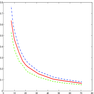
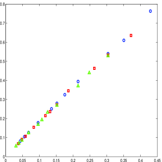
Figure 1: $Y-$axis: Coherence $\tau_{n}$. $X-$axis: $\sqrt{n}$ (left) or $\sqrt{\frac{log(p)}{n}}$ (right) for $p=100$ (dashdot line or triangle -green), $p=1000$ (solid line or square -red), $p=10000$ (dash line or circle -blue). $K=500$

The design matrix $\Phi$ is first defined with i.i.d. gaussian variables. Figure 1 (left) shows the evolution of the empirical coherence $\tau_{n}$ function of $\sqrt{n}$ for $p=100$, $1000$, or $10000$. Each coherence shown in the graph is the average of $K=500$ coherence values computed for different $\Phi$ matrix simulated at random over the $K$ replications. As the number of observations increases to $n=5000$ ($\sqrt{5000}\simeq 70.7$), the coherence tends to be quite small ($\tau_{n}=0.1$) independently of the number of variables $p$. For a small number of observations, the coherence takes pretty high values, much higher as the number of predictors increases. For example, for $n=250$ ($\sqrt{250}\simeq 15.8$)

$$p=100\mapsto\tau_{n}=0.25,\quad p=100\mapsto\tau_{n}=0.30,\quad p=1000\mapsto\tau_{n}=0.35.$$

A difference of $15\%$ is observed between the coherences computed for $p=1000$ and $p=100$, or $p=1000$ and $p=10000$. Figure 1 (right) shows the evolution of the coherence as a function of $\sqrt{log(p)/n}$ which allows to compute the constant $c$ introduced in Theorem 1.

Since we are interested by quantifying the performances of LOL in an overwhelming majority of cases ($n$, $p$ varying), the impact of the level of indeterminacy and of the sparsity rate are studied: $\delta$ is varying from $0$ to $0.9$ by $0.05$ step and $\rho$ is varying from $0.01$ to $0.16$ by 20 steps. We fixe $p=1000$ and $n=250$ for this specific study.

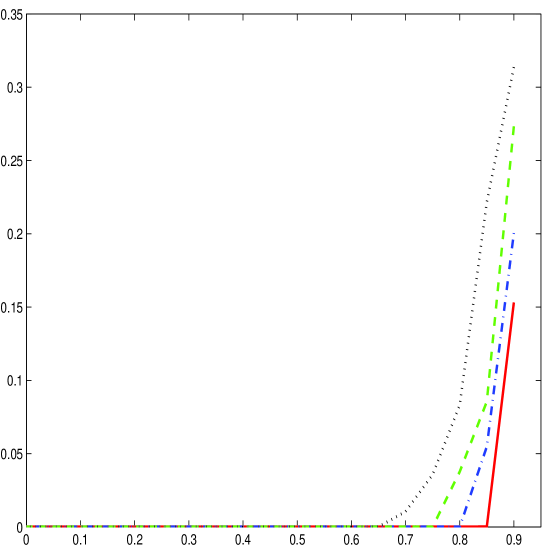
Figure 2: $X-$axis: indeterminacy level $\delta$, $Y-$axis: relative prediction error. $S=10$ (solid line-red); $S=12$ (dashdot line-blue); $S=15$ (dash line-green); $S=20$ (dot line-black). $SNR=5$.

Influence of the indeterminacy level: Figure 2 studies the performances of LOL when the indeterminacy level is varying ($p=1000$ fixed, $n$ varying), for different sparsity values ($S=10,12,15,20$). The error of prediction $E_{Y}$ increases continuously with the indeterminacy $\delta$, as the number of observations decreases compared to the number of variables. For a given value of $\delta$, $E_{Y}$ decreases as the sparsity does. For $\delta\leq 0.75$, the prediction error is weak, below $5\%$. When the number of available observations is at least higher than half of the number of potential predictors ($\delta<0.5$), the prediction error is negligible: the quality of LOL is in this case exceptionally good. For a given number of observations and potential predictors, the prediction is more accurate as the sparsity rate decreases. For a fixed number of observations, regarding the joint values of both indeterminacy and sparsity parameters, the errors tends to be null as $\delta$ and/or $\rho$ are decreasing.

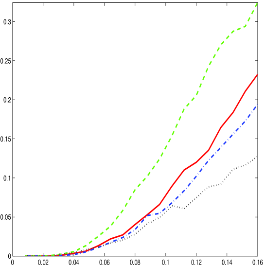
Figure 3: $X-$axis: sparsity rate $\rho$, $Y-$axis: relative prediction error. $\delta=0.4$ (dot line-black); $\delta=0.7$ (dashdot line-blue); $\delta=0.75$ (solid line-red); $\delta=0.875$, (dashed line-green). $SNR=5$.

Influence of the sparsity rate: Figure 3 illustrates the performances of LOL for prediction when the sparsity rate is varying for four levels of indeterminacy ($\delta=0.4,0.7,0.75,0.875$). For small values of the sparsity rate ($\rho\leq 5\%$), the prediction error is very good (less than $5\%$). For an extreme level of sparsity ($\rho\leq 2\%$), the performances are excellent. As observed before, for a given sparsity rate value, the performances are improved as the indeterminacy level is decreasing.

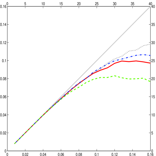
Figure 4: LOL Sparsity Estimation ( $\rho$: bottom, left; $S$: right, top). $\delta=0.875$ (dashed line-green); $\delta=0.75$ (solid line-red); $\delta=0.7$ (dashdot line-blue); $\delta=0.4$ (dot line-black).

Estimation of the Sparsity $S$: Figure 4 shows the estimation of the sparsity provided by LOL as a function of the effective sparsity $S$. For small $S$ ($\rho\leq 5\%$), LOL is excellent because it estimates exactly (with no error) the sparsity $S$ for all the studied indeterminacy levels. As the sparsity $S$ increases, LOL underestimates the parameter $S$. For a given sparsity value, the underestimation becomes weaker as the indeterminacy level $\delta$ decreases. Comparing Figure 3 and Figure 4, we observe that the estimation sparsity is obviously linked to the prediction error which is not a surprise.

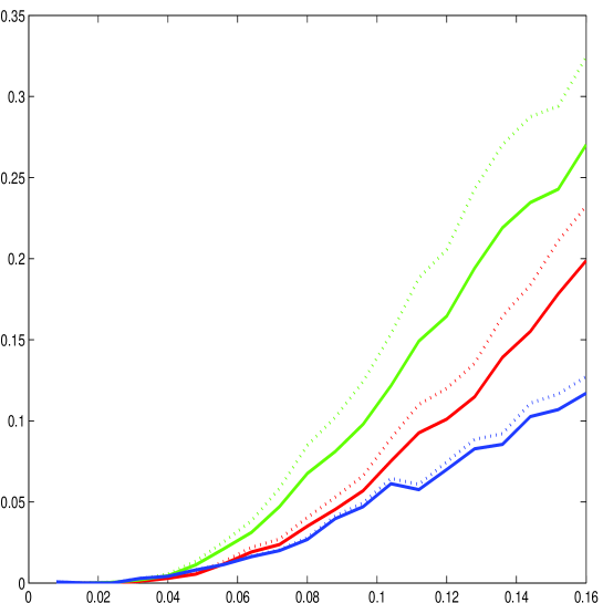
Figure 5: $X-$axis: sparsity rate $\rho$. $Y-$axis: relative prediction errors for LOL (dot lines) and LOL+ (solid lines). $\delta=0.4$ (blue color); $\delta=0.75$ (red color); $\delta=0.875$ (green color). The regressors are Gaussian of size $n=250$. $SNR=5$.

Estimation of the coefficients: Figure 5 presents the improvements provided by LOL⁺ compared to LOL as a function of sparsity rate for the prediction error. For all indeterminacy and sparsity values, the prediction error decreases using LOL⁺ procedure instead of LOL. The improvements are stronger as both sparsity rate and indeterminacy level increase. The improvements for the prediction error are observed as $\rho$ increases given all studied indeterminacy levels $\delta$. Obviously, the estimated sparsity in the same for both procedures LOL and LOL⁺.

Ultra high dimension: Table 3 shows the prediction error for ultra high dimension as $p=5000$, $p=10000$; $p=20000$ and for two different values of $n=400$ and $n=800$. For small sparsity levels ($S=5$, $10$, $20$), the performances are similar even in a very high dimension as $p=20000$. As in the previous studies in smaller dimension, for higher sparsity levels ($S=40$, $60$), the performances decrease as the sparsity level or the indeterminacy increases.

6.4 Influence of dependence for gaussian design matrices

In the simulations, all the predictors do not have the same influence because some predictors are directly involved in the model and some others not. Different type of dependency between the predictors can also be distinguished: dependency between two predictors involved (or not involved) in the real underlying model, and dependencies between two predictors: one involved in the model, the other not. These dependencies have not the same impact on the results. In order to simulate all possible dependencies, we first extract a $\Phi_{n,2S}$ sub matrix of $\Phi$ defined by concatenating vertically the $S$ columns of the predictors included in the model (and associated with non zero coefficients), and $S$ columns between the $(p-S+1)$ predictors chosen at random not included in the model. $W_{1}$ is the associated correlation matrix of $\Phi_{n,2S}$. A new correlation matrix $W_{2}$ is then built by choosing randomly $5\%$ or $20\%$ of the correlations in $W_{1}$ and replacing their original value with random values of the form $(-1)^{b}u$, where $b$ is drawn from a Bernoulli distribution with parameter $0.5$ and $u$ from an uniform distribution between $[0.90;0.95]$ such a way that $W_{2}$ presents some high correlations between the $2S$ selected predictors. Since the correlation matrix of the $2S$ columns of $Z:=\Phi_{n,2S}W_{1}^{-\frac{1}{2}}W_{1}^{\frac{1}{2}}$ is then $W_{2}$, we replace the previously removed columns of $\Phi$ by the columns of $Z$.

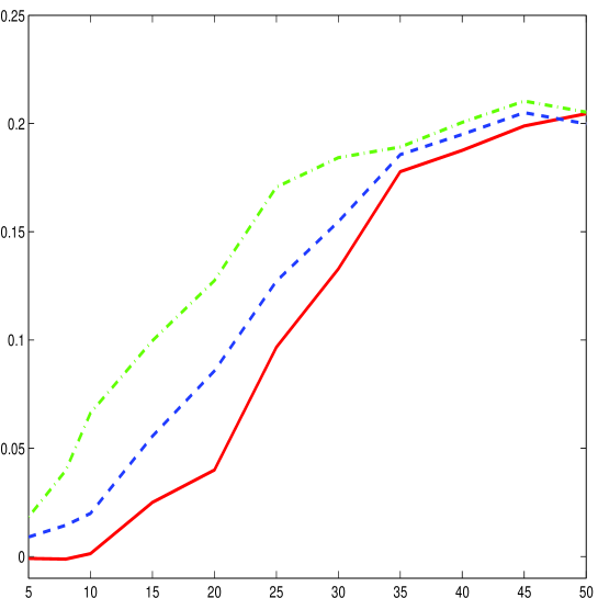
Figure 6: $X-$axis: sparsity $S$. $Y-$axis: relative prediction errors, for LOL with independent regressors (solid line-red) and dependent regressors ($5\%$ of dependency, dashdot line-blue; $20\%$, dashed line-blue). $p=1000$, $n=250$, $K=100$. $SNR=5$.

Figure 6 compares the prediction error for both dependent and independent cases. As expected, some dependency between the predictors damages the performances of LOL. When the sparsity increases, the impact of dependency seems to play a lower impact on the prediction error.

6.5 Impact of the family distribution of the design matrix

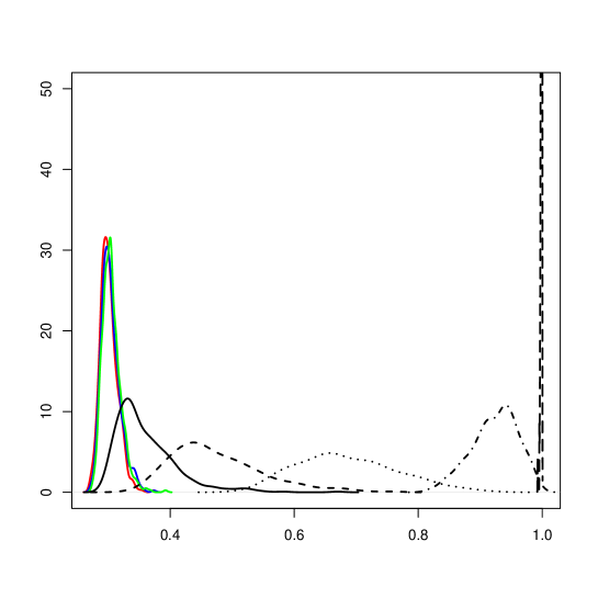
Figure 7: Empirical densities of the coherence $\tau_{n}$. The regressors are Gaussien (solid line-red); uniform (solid line-blue); Bernoulli (solid line-green); Student $5,4,3,2,1$ black lines from left to right. $n=250,p=1000$.

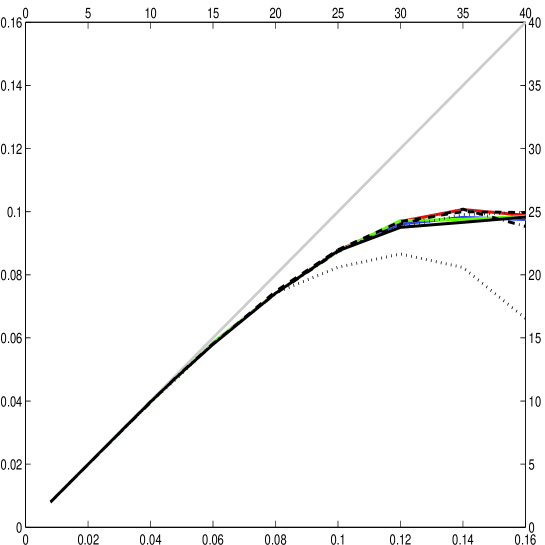
Figure 8: LOL Sparsity estimation for different distributions for the predictors. $Gauss$ (solid line-red); $Uniform$ (solid line-blue); $Bernoulli$: (solid line-green); T(2-5) (black-lines); T(1) (dot black line). $n=250$, $p=1000$. ($K=200$)

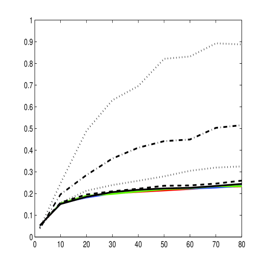
Figure 9: $X-$axis: sparsity $S$. $Y-$axis: Coherence $\tau_{n}$ computed for the $N$ selected Leaders. $Gauss$ (solid line-red); $Uniform$ (solid line-blue); $Bernoulli$: (solid line-green); T(1) (dot line-black). $n=250$, $p=1000$. ($K=200$)

In this section, we investigate the impact of the distribution in a design matrix with i.i.d. entries. Eight different distributions are studied: Gaussian ($N(0,1)$), Uniform ($U[-1,1]$), Bernoulli ($B\{-1,+1\}$) and Student ($T(m)$ with $m\in\{5,4,3,2,1\}$). Figure 7 shows the empirical density of the coherence $\tau_{n}$ computed for each law ($n=250$). Similar distributions are observed for Gaussian, Uniform or Bernoulli laws with a mode of the coherence equal to $\tau_{n}=0.30$. For Student’s families, a shift of the mode of the empirical distributions can be observed from left to right equaled to 0.36 for $T(5)$, 0.47 for T(4), 0.68 for T(3), 0.92 for T(2) to 0.99 for T(1). The prediction errors computed using LOL are presented in Table 1. For all distributions, the prediction errors increase with sparsity in average and in variability. As expected, regarding the coherence value, similar prediction errors are provided for Gaussian, Uniform, or Bernoulli laws. For the Student distributions $T(m)$ with parameter $m\geq 2$, the prediction results are also similar to Gaussian distribution. The Student distribution with $m=1$ shows much higher prediction errors both in average and variability. Figure 8 studies the estimation of sparsity using LOL as a function of the sparsity rate $\rho$. All the curves, except the one for the Student law T(1), are confounded and show similar behavior as the one observed for gaussian predictors (see Figure 4 for $\delta=0.25$). LOL provides similar results for Gaussian, Uniform, Bernoulli, or Student laws, $T(m)$ with $m$ large enough. It is amazing to observe that the procedure works fine even when the empirical coherence $\tau_{n}$ reaches large values. However, LOL does not work fine for heavy tailed variables as for $T(1)$. These results can be explained analyzing Figure 9 which shows the coherence of the matrix restricted to the $N$ selected leaders. This restricted coherence is much lower than the coherence computed on all the predictors. For the Student $T(1)$ law, $\tau_{n}=0.99$ (see Figure 7) while the coherence restricted to the leaders is $0.3$ (see Figure 9 by instance for $S=10$). LOL provides also good results even when the global coherence approaches $1$. It seems then that the practical results are much more optimistic than the theoretical ones, although they show deteriorations under high coherence. Conclusions would be that it could be interesting to find new measures of collinearity to reflect better the performances of the method. This is true in general for all the methods concerned with high dimension.

6.6 Comparison with other two-step procedures

In this part, the performances of LOL are compared with the performances of other two-step procedures which have been practically studied. The first one referred as SIS-Lasso is coming from Fan and Lv (2008): the selection step called SIS is followed by the Lasso procedure. The second one called Lasso-Reg, is proposed in Candès and Plan (2009). First, the Lasso algorithm performs the selection of the leaders and then, the coefficients are estimated with a regression. For simplicity of the presentation, we do not include the results provided by greedy algorithms.

The performances of the three procedures (LOL, SIS-Lasso, Lasso-Reg) are here studied over a large range of sparsity in order to cover previous results already presented in Fan and Lv (2008) and Candès and Plan (2009) for different sparsity. The number of initial predictors is $p=1000$ and the number of observations $n=200$. This experimental design allows us to analyze extremely small sparsity values ($10\leq S\leq 20$) (as in Fan and Lv (2008)) as well as values as large as $S=60$ (as in Candès and Plan (2009)). For the Lasso procedures, the regularization parameter is chosen by cross validation. Different signal over noise ratio are studied ($SNR=10$, $5$, $2$).

Table 2 presents the relative prediction error as defined for i.i.d. gaussian matrices but similar results are obtained with uniform, or Bernoulli distribution. Different cases of signal over noise ratio are studied ($SNR=10,5,2$). The performances of the procedures appear to depend on the sparsity and on the signal over noise ratio. For small sparsity levels, ($S=10$), all the procedures perform extremely well and the relative prediction error is similar to the inverse of the signal over noise ratio. For middle sparsity levels ($20\leq S\leq 30$), Lasso-Reg performs better than the others ones when the signal over noise ratio is high ($SNR=10$ or $5$). In this case, Lasso-Reg seems to be more efficient to select (during the first step) the leaders than both SIS-Lasso and LOL. For a low signal over noise ratio ($SNR=2$), LOL performs better than Lasso-Reg. The performances of SIS-Lasso and LOL are globally similar.

For largest values of the sparsity level $S\geq 50$, it appears that SIS-Lasso and LOL are better than Lasso-Reg for middle values of the signal over noise ratio.

We conclude that LOL has a special gain over the other procedures when the SNR is small or when the sparsity $S$ is high.

6.7 LOL in Boston

In order to illustrate the performances of LOL on real data, we revisit the Boston Housing data (available from the UCI machine learning data base repository: http://archive.ics.ucfi.edu/ml/) by fitting predictive models using LOL. The original Boston Housing data have one continuous target variable $Y$ (the median value of owner-occupied homes in USD) and $p_{0}=13$ predictive variables over $n=506$ observations which are randomly split into two subsets: one training set with $75\%$ of observations and one test set with the remaining $25\%$ observations.

In view to test our procedure, we consider the linear regression method as a benchmark and denote $E^{Reg}$ the prediction error computed on the test set while the estimated model is computed on the training set.

The data are ’dived’ in a high dimensional space of size $p=2113$ by adding $300$ independent random variables of seven different laws: Normal, lognormal, Bernoulli, Uniform, exponential with parameter 2, Student $T(2)$, $T(1)$ in equal proportion. This set of laws is chosen to mimic the different underlaying laws of the 13 original variables. LOL is applied on the training set and the error of prediction $E^{LOL}$ is computed on the test set. This procedure is repeated $K=100$ times using re sampling, and the prediction errors are then averaged to compute the performances on the training and test sets. Observe that in this example, the indeterminacy level and the sparsity rate are quite low equal to $\delta=0.18$ and $\rho=0.034$. The coherence is quite high equal to $\tau_{n}=0.98$.

The results are the following

$$E^{LOL}=0.245(0.05)\quad\mbox{ and }\quad E^{Reg}=0.266(0.04)$$

and LOL appears to work in this case very well because similar prediction errors are obtained even from a high dimensional space $p=2113$ as using a regular linear regression in $p_{0}=13$ dimensions.

7 Proofs

First, we state preliminary results and next we prove Theorem 2 and Theorem 1 as a consequence of Theorem 2. The proofs of the preliminaries are postponed in the appendix.

For any subset of indices ${\mathcal{I}}\subset\{1,\ldots,p\}$, $V_{\mathcal{I}}$ denotes the subspace of $\mathbb{R}^{n}$ spanned by the columns of the extracted matrix $\Phi_{|\mathcal{I}}$ and $P_{V_{\mathcal{I}}}$ denotes the projection over $V_{\mathcal{I}}$ (in euclidean sense in $\mathbb{R}^{n})$. Set $\bar{\alpha}(\mathcal{I})$ the vector of $\mathbb{R}^{\#(\mathcal{I})}$ such that $\Phi_{|\mathcal{I}}\bar{\alpha}(\mathcal{I}):=P_{V_{\mathcal{I}}}[\Phi\alpha]$. Obviously, as soon as $\#(\mathcal{I})\leq N$, we get

$$\bar{\alpha}(\mathcal{I})=(\Phi_{|\mathcal{I}}^{t}\Phi_{|\mathcal{I}})^{-1}\Phi_{|\mathcal{I}}^{t}\Phi\alpha.$$

As well, set $\hat{\alpha}(\mathcal{I})$ such that $\Phi_{|\mathcal{I}}\hat{\alpha}(\mathcal{I}):=P_{V_{\mathcal{I}}}(Y)$.

7.1 Preliminaries

The preliminaries contain three essential results for the subsequent proof. The first proposition describes the algebraic behavior of the euclidean norm of $\hat{\alpha}({\mathcal{B}})-\alpha$ when the vector is restricted to a (small) set of indices. The second lemma is a consequence of the RIP property and gives an algebraic equivalent for the projection norm of vectors over spaces of small dimensions. The second proposition (third result) describes the concentration property for projections norms of the vector of errors. This proposition is our major ingredient for proving all the exponential bounds. Note that it also incorporates the case where the projection has a possibly random range.

Proposition 1

Let $\mathcal{I}$ be a subset of the leaders indices set ${\mathcal{B}}$. Then

$$\sum_{\ell\in\mathcal{I}}(\widehat{\alpha_{\ell}}({\mathcal{B}})-\alpha_{\ell})^{2} \leq\kappa(\alpha)\#(\mathcal{I})\tau_{n}^{2}\left(1+\|P_{V_{{\mathcal{B}}}}[\varepsilon]\|_{n}^{2}\right)+\frac{3c_{0}^{2}}{1-\nu}\frac{S}{n}+\frac{3}{1-\nu}\|P_{V_{\mathcal{I}}}[\varepsilon]\|_{n}^{2}$$

where

$$\kappa(\alpha)=\frac{3(5+\nu)}{(1-\nu)}\|\alpha\|^{2}_{l^{1}(p)}\vee\frac{3}{(1-\nu)}.$$

Lemma 2

Let $\mathcal{I}$ be a subset of $\{1,\ldots,p\}$ satisfying $\#(\mathcal{I})\leq N$. Then, for any $x\in\mathbb{R}^{n}$, we get

$$(1+\nu)^{-1}\sum_{\ell\,\in\mathcal{I}}\;\frac{1}{n}\left(\sum_{i=1}^{n}x_{i}\Phi_{i\ell}\right)^{2}\leq\|P_{V_{\mathcal{I}}}x\|_{l^{2}(n)}^{2}\leq(1-\nu)^{-1}\sum_{\ell\,\in\mathcal{I}}\;\frac{1}{n}\left(\sum_{i=1}^{n}x_{i}\Phi_{i\ell}\right)^{2}\,.$$

Proposition 2

Let $\mathcal{I}$ be a non random subset of $\{1,\ldots,p\}$ such that $\#(\mathcal{I})\leq n_{\mathcal{I}}$, where $n_{\mathcal{I}}$ is a deterministic quantity, then

$$P\left(\frac{1}{\sigma^{2}}\|P_{V_{\mathcal{I}}}[\varepsilon]\|_{n}^{2}\geq\mu^{2}\right) \leq\exp\left(-n\mu^{2}/16\right)$$ (15)

for any $\mu$ such that $\mu^{2}\geq 4\,n_{\mathcal{I}}/n$. If now $\mathcal{I}$ is a random subset of $\{1,\ldots,p\}$ such that $\#(\mathcal{I})\leq n_{\mathcal{I}}$, where $n_{\mathcal{I}}$ is a deterministic quantity, then (15) is still true but for any $\mu$ such that $\mu^{2}\geq 16\,n_{\mathcal{I}}\log{p}/n$.

Proposition 1 and Proposition 2 are proved in the appendix as well as Lemma 2.

7.2 Proof of Theorem 2

For sake of simplicity, and without loss of generality, we assume that the $N$ largest $\alpha_{\ell}$’s have their indices in $\{1,\ldots,N\}$. We have

$$d(\hat{\alpha}^{*},\alpha) \leq\|u\|_{n}+\|\sum_{\ell=1}^{p}(\hat{\alpha}_{\ell}^{*}-\alpha_{\ell})\Phi_{\bullet\ell}\|_{n}\;.$$

Recall that ${\mathcal{B}}$ is the set of the indices of the leaders. Then

$$\|\sum_{\ell=1}^{p}(\hat{\alpha}_{\ell}^{*}-\alpha_{\ell})\Phi_{\bullet\ell}\|_{n} \leq\|\sum_{\ell=1}^{p}{\mathbb{I}}\{\ell\in{\mathcal{B}}\}(\hat{\alpha}_{\ell}^{*}-\alpha_{\ell})\Phi_{\bullet\ell}\|_{n}+\|\sum_{\ell=1}^{p}{\mathbb{I}}\{\ell\not\in{\mathcal{B}}\}\,\alpha_{\ell}\Phi_{\bullet\ell}\|_{n}$$

$$:=I\;(\mbox{In})\;+O\;(\mbox{Out})\;.$$

We split $I$ into four terms by observing that :

$$1 ={\mathbb{I}}\{|\hat{\alpha}_{\ell}({\mathcal{B}})|\geq\lambda_{n}(2)\}\big{\{}{\mathbb{I}}\{|\alpha_{\ell}|\geq\lambda_{n}(2)/2\}+{\mathbb{I}}\{|\alpha_{\ell}|<\lambda_{n}(2)/2\}\big{\}}$$

$$+{\mathbb{I}}\{|\hat{\alpha}_{\ell}({\mathcal{B}})|<\lambda_{n}(2)\}\big{\{}{\mathbb{I}}\{|\alpha_{\ell}|\geq 2\lambda_{n}(2)\}+{\mathbb{I}}\{|\alpha_{\ell}|<2\lambda_{n}(2)\}\big{\}}.$$

It follows that

$$I \leq\left(\|\sum_{\ell=1}^{N}\;{\mathbb{I}}\{\ell\in{\mathcal{B}}\}(\hat{\alpha}_{\ell}^{*}-\alpha_{\ell})\Phi_{\bullet\ell}\;{\mathbb{I}}\{|\alpha_{\ell}|\geq\lambda_{n}(2)/2\}\;{\mathbb{I}}\{|\hat{\alpha}_{\ell}({\mathcal{B}})|\geq\lambda_{n}(2)\}\|_{n}\right.$$

$$\hskip 56.9055pt+\left.\|\sum_{\ell=1}^{N}\;{\mathbb{I}}\{\ell\in{\mathcal{B}}\}\alpha_{\ell}\Phi_{\bullet\ell}\;{\mathbb{I}}\{|\alpha_{\ell}|\geq 2\lambda_{n}(2)\}\;{\mathbb{I}}\{|\hat{\alpha}_{\ell}({\mathcal{B}})|<\lambda_{n}(2)\}\|_{n}\right)$$

$$+\left(\|\sum_{\ell=1}^{p}\;{\mathbb{I}}\{\ell\in{\mathcal{B}}\}(\hat{\alpha}_{\ell}^{*}-\alpha_{\ell})\Phi_{\bullet\ell}\;{\mathbb{I}}\{|\alpha_{\ell}|<\lambda_{n}(2)/2\}\;{\mathbb{I}}\{|\hat{\alpha}_{\ell}({\mathcal{B}})|\geq\lambda_{n}(2)\}\|_{n}\right.$$

$$\hskip 56.9055pt+\left.\|\sum_{\ell=1}^{p}{\mathbb{I}}\{\ell\in{\mathcal{B}}\}\alpha_{\ell}\Phi_{\bullet\ell}\;{\mathbb{I}}\{|\alpha_{\ell}|<2\lambda_{n}(2)\}\;{\mathbb{I}}\{|\hat{\alpha}_{\ell}({\mathcal{B}})|\leq\lambda_{n}(2)\}\|_{n}\right)$$

$$:=IBB\;(\mbox{InBigBig})\;+ISB\;(\mbox{InSmallBig})\;+IBS\;(\mbox{InBigSmall})\;+ISS\;(\mbox{InSmallSmall})\;.$$

Note that because of Assumption (10), the coefficients such that $|\alpha_{\ell}|\geq\lambda_{n}(2)/2$ necessarily have their indices less than $N$, so some terms in the above sum have their summation up to $N$, some others up to $p$. This makes an important difference in the sequel because Lemma 1 can be used in the first case. Recall the definition of the $\widetilde{\alpha}_{\ell}$’s given in Algorithm 3.1

$$\widetilde{\alpha}_{\ell} := \frac{1}{n}\,\sum_{i=1}^{n}Y_{i}\Phi_{i\ell}.$$

We have

$$O \leq\|\sum_{\ell=N+1}^{p}\;{\mathbb{I}}\{\ell\not\in{\mathcal{B}}\}\,\,\alpha_{\ell}\Phi_{\bullet\ell}\|_{n}+\|\sum_{\ell=1}^{N}\;{\mathbb{I}}\{\ell\not\in{\mathcal{B}}\}\,\alpha_{\ell}\Phi_{\bullet\ell}\;\|_{n}$$

$$\leq\|\sum_{\ell=N+1}^{p}\;{\mathbb{I}}\{\ell\not\in{\mathcal{B}}\}\,\,\alpha_{\ell}\Phi_{\bullet\ell}\|_{n}+\|\sum_{\ell=1}^{N}\;{\mathbb{I}}\{\ell\not\in{\mathcal{B}}\}\,\alpha_{\ell}\Phi_{\bullet\ell}\;{\mathbb{I}}\{|\alpha_{\ell}|\leq 2\lambda_{n}(1)\}\|_{n}$$

$$+\|\sum_{\ell=1}^{N}\;{\mathbb{I}}\{\ell\not\in{\mathcal{B}}\}\,\alpha_{\ell}\Phi_{\bullet\ell}\;{\mathbb{I}}\{|\alpha_{\ell}|\geq 2\lambda_{n}(1)\}\;{\mathbb{I}}\{|\widetilde{\alpha}_{\ell}|\leq\lambda_{n}(1)\}\|_{n}$$

$$+\|\sum_{\ell=1}^{N}\;{\mathbb{I}}\{\ell\not\in{\mathcal{B}}\}\,\alpha_{\ell}\Phi_{\bullet\ell}\;{\mathbb{I}}\{|\alpha_{\ell}|\geq 2\lambda_{n}(1)\}\;{\mathbb{I}}\{|\widetilde{\alpha}_{\ell}|\geq\lambda_{n}(1)\}\|_{n}$$

$$:=Ob\;(\mbox{OutBias})\;+OS\;(\mbox{OutSmall})\;+OBS\;(\mbox{OutBigSmall})\;+OBB\;(\mbox{OutBigBig})\;$$

Using the Assumption (13) on the errors, we get

$$\|u\|_{n} \leq\sup_{i=1,\ldots,n}|u|\leq c_{0}\sqrt{\frac{S}{n}}.$$

We deduce that for any $\eta$ such that

$$\eta^{2} >2\,c_{0}^{2}\frac{S}{n},$$ (16)

$$P\left(d(\hat{\alpha}^{*},\alpha)\geq\eta\right) \leq P\left(I+O\geq\eta/2\right)$$

$$\leq P\left(IBB+ISB+IBS+ISS\geq\eta/4\right)+P\left(OS+OBB+OBS+Ob\geq\eta/4\right).$$

Our aim is to prove that each probability term is bounded by $\exp-\gamma n\eta^{2}$ for any

$$\eta^{2}\geq D\left(\frac{S\log{p}}{n}\vee S\tau_{n}^{2}\right)$$

where the constants $\gamma$ and $D$ have to be determined. To do this, basically, we study each term separately and prove that (up to constants) either it can be directly bounded, or it reduces to a random term whose probability of excess can be bounded using Proposition 2.

7.2.1 Study of $IBB$ and $ISB$

Denote by $\mathcal{T}$ the (non random) set of indices $\{\ell=1,\ldots,N,\,|\alpha_{\ell}|\geq\lambda_{n}(2)/2\}$ which verifies $\#\mathcal{T}\leq S$ by Assumption 10. Observe that

$$\left\{\begin{array}[]{l}|(\hat{\alpha}({\mathcal{B}}))_{\ell}|<\lambda_{n}(2)\\ |\alpha_{\ell}|>2\lambda_{n}(2)\end{array}\right. \Longrightarrow |(\hat{\alpha}({\mathcal{B}}))_{\ell}|<\lambda_{n}(2)<|\alpha_{\ell}-(\hat{\alpha}({\mathcal{B}}))_{\ell}|$$

Using Lemma 1, we deduce that

$${ISB^{2}} \leq (1+\nu)\sum_{\ell\in\mathcal{T}\cap{\mathcal{B}}}|(\hat{\alpha}({\mathcal{B}}))_{\ell}+(\alpha_{\ell}-(\hat{\alpha}({\mathcal{B}}))_{\ell})|^{2}\;{\mathbb{I}}\{|(\hat{\alpha}({\mathcal{B}}))_{\ell}|\leq|\alpha_{\ell}-(\hat{\alpha}({\mathcal{B}}))_{\ell}|\}\;{\mathbb{I}}\{|\alpha_{\ell}|\geq 2\lambda_{n}(2)\}$$

$$\leq 4(1+\nu)\sum_{\ell\in\mathcal{T}\cap{\mathcal{B}}}(\alpha_{\ell}-(\hat{\alpha}({\mathcal{B}}))_{\ell})^{2}.$$

Using again Lemma 1, it follows that

$${ISB^{2}}+IBB^{2} \leq 5(1+\nu)\sum_{\ell\in\mathcal{T}\cap{\mathcal{B}}}(\alpha_{\ell}-(\hat{\alpha}({\mathcal{B}}))_{\ell})^{2}.$$

We apply Proposition 1

$${ISB^{2}}+IBB^{2} \leq 5(1+\nu)\left(\kappa(\alpha)S\tau_{n}^{2}\left(1+\,\|P_{V_{{\mathcal{B}}}}[\varepsilon]\|_{n}^{2}\right)+\frac{3c_{0}^{2}}{1-\nu}\frac{S}{n}+\frac{3}{1-\nu}\|P_{V_{\mathcal{T}}}[\varepsilon]\|_{n}^{2}\right).$$

We use now Proposition 2: first with the non random set $\mathcal{T}$ satisfying $\#(\mathcal{T})\leq S$, secondly with the random set ${\mathcal{B}}$ such that $\#({\mathcal{B}})\leq N$. For this second part, we use the last part of Proposition 2, which yields an additional logarithmic factor. We obtain

$$P\left(IBB+ISB\geq\eta/8\right) \leq P\left(\frac{1}{\sigma^{2}}\,\|P_{V_{\mathcal{T}}}\varepsilon\|_{n}^{2}\geq\eta^{2}\,(1-\nu)/(7680(1+\nu)\sigma^{2})\right)$$

$$+P\left(\frac{1}{\sigma^{2}}\,\|P_{V_{\mathcal{B}}}\varepsilon\|_{n}^{2}\geq\eta^{2}(S\tau_{n}^{2})^{-1}/(2560(1+\nu)\kappa(\alpha)\sigma^{2})\right)$$

$$\leq 2\exp\left\{-n\eta^{2}(1-\nu)/(30720(1+\nu)\sigma^{2}\right)$$

since $S\leq N=\nu/\tau_{n}$ and as soon as

$$\eta^{2} \geq 2560\left((1+\nu)\kappa(\alpha)S\tau_{n}^{2}\vee\frac{c_{0}^{2}}{1-\nu}\frac{S}{n}\right)\vee 30720\frac{(1-\nu)}{(1+\nu)}\sigma^{2}\frac{S}{n}$$

$$\hskip 28.45274pt\vee 40960\nu(1+\nu)\nu\,\kappa(\alpha)\sigma^{2}\frac{S\tau_{n}\,\log{p}}{n}.$$ (18)

7.2.2 Study of $Ob$

Since the $\Phi_{\bullet\ell}$’s are normalized vectors and because of the definition of the coherence, we get

$$Ob \leq \|\sum_{\ell\geq N+1}\alpha_{\ell}\Phi_{\bullet\ell}\|_{n}$$

$$\leq \left[\sum_{\ell\geq N+1}\alpha_{\ell}^{2}+\tau_{n}\left(\sum_{\ell\geq N+1}|\alpha_{\ell}|\right)^{2}\right]^{1/2}$$

$$\leq \left[\sum_{\ell\geq N+1}\alpha_{\ell}^{2}\,{\mathbb{I}}\{|\alpha_{\ell}|\leq\lambda_{n}(2)/2\}+\tau_{n}\left(\sum_{\ell\geq N+1}|\alpha_{\ell}|\right)^{2}\right]^{1/2}.$$

As $\lambda_{n}(2)\leq\lambda_{n}(1)$ and using Assumption (12) and Assumption (11), we obtain

$$Ob\leq\,(c_{1}+c_{2})\sqrt{\frac{S\log{p}}{n}}$$

which implies that $Ob\leq\eta/16$ as soon as

$$\eta^{2} >256(c_{1}+c_{2})^{2}\;\frac{S\log{p}}{n}.$$ (19)

7.2.3 Study of $ISS$ and $OS$

As $\lambda_{n}(1)\geq\lambda_{n}(2)$, using successively Lemma 1 and Assumption (12), we have

$$ISS \leq Ob+\|\sum_{\ell=1}^{N}{\mathbb{I}}\{\ell\in{\mathcal{B}}\}\alpha_{\ell}\Phi_{\bullet\ell}\;{\mathbb{I}}\{|\alpha_{\ell}|\leq 2\lambda_{n}(2)\}\;{\mathbb{I}}\{|\hat{\alpha}_{\ell}({\mathcal{B}})|\leq\lambda_{n}(2)\}\|_{n}$$

$$\leq Ob+(1+\nu)^{1/2}\,\left(\sum_{\ell=1}^{N}\alpha_{\ell}^{2}\;{\mathbb{I}}\{|\alpha_{\ell}|\leq 2\lambda_{n}(1)\}\right)^{1/2}$$

$$\leq(c_{1}+c_{2})\sqrt{\frac{S\log{p}}{n}}+(1+\nu)^{1/2}c_{2}\sqrt{\frac{S\log{p}}{n}}.$$

This implies that $ISS\leq\eta/16$ as soon as

$$\eta^{2} >512\,\left((c_{1}+c_{2})^{2}+(1+\nu)c_{2}^{2}\right)\,\frac{S\log{p}}{n}.$$ (20)

In the same way, $OS\leq\eta/16$.

7.2.4 Study of $OBS$

Using the model and the definition of $\widetilde{\alpha_{\ell}}$ given in Algorithm 3.1, we get

$$\widetilde{\alpha_{\ell}}=\frac{1}{n}\sum_{i=1}^{n}[\sum_{m=1}^{p}\alpha_{m}\Phi_{im}+u_{i}+\varepsilon_{i}]\,\Phi_{i\ell}.$$

Since $\Phi$ has normalized columns, we can write

$$\alpha_{\ell}=\frac{1}{n}\sum_{i=1}^{n}\alpha_{\ell}\Phi_{i\ell}\Phi_{i\ell}$$

which implies that

$$|\widetilde{\alpha_{\ell}}-\alpha_{\ell}| \leq \left|\frac{1}{n}\sum_{i=1}^{n}\left(\sum_{m=1}^{p}\alpha_{m}\Phi_{im}\Phi_{i\ell}-\alpha_{\ell}\Phi_{i\ell}\Phi_{i\ell}\right)\right|+\left|\frac{1}{n}\sum_{i=1}^{n}u_{i}\Phi_{i\ell}\right|+\left|\frac{1}{n}\sum_{i=1}^{n}\varepsilon_{i}\Phi_{i\ell}\right|$$ (21)

$$\leq \left|\sum_{m=1,m\not=\ell}^{p}\alpha_{m}\,\frac{1}{n}\sum_{i=1}^{n}\left(\Phi_{im}\Phi_{i\ell}\right)\right|+\left|\frac{1}{n}\sum_{i=1}^{n}u_{i}\Phi_{i\ell}\right|+\left|\frac{1}{n}\sum_{i=1}^{n}\varepsilon_{i}\Phi_{i\ell}\right|$$

$$\leq \sum_{m=1,m\not=\ell}^{p}|\alpha_{m}|\tau_{n}+\left|\frac{1}{n}\sum_{i=1}^{n}u_{i}\Phi_{i\ell}\right|+\left|\frac{1}{n}\sum_{i=1}^{n}\varepsilon_{i}\Phi_{i\ell}\right|.$$

Recall that $\lambda_{n}(1)\geq\lambda_{n}(2)$. We get

$${\mathbb{I}}\{|\widetilde{\alpha_{\ell}}|<\lambda_{n}(1)\}\;{\mathbb{I}}\{|\alpha_{\ell}|\geq 2\lambda_{n}(1)\}\quad\leq\quad{\mathbb{I}}\{|\alpha_{\ell}-\widetilde{\alpha_{\ell}}|\geq\lambda_{n}(1)\geq|\widetilde{\alpha_{\ell}}|\}\;{\mathbb{I}}\{|\alpha_{\ell}|\geq\lambda_{n}(2)/2\}.$$

Hence, using Lemma 1, it follows

$$OBS^{2} \leq (1+\nu)\sum_{\ell=1}^{N}(\alpha_{\ell}-\widetilde{\alpha_{\ell}}+\widetilde{\alpha_{\ell}})^{2}\;{\mathbb{I}}\{|\alpha_{\ell}-\widetilde{\alpha_{\ell}}|\geq\lambda_{n}(1)\geq|\widetilde{\alpha_{\ell}}|\}\,{\mathbb{I}}\{|\alpha_{\ell}|\geq\lambda_{n}(2)/2\}$$ (22)

$$\leq 4(1+\nu)\sum_{\ell=1}^{N}(\alpha_{\ell}-\widetilde{\alpha_{\ell}})^{2}\,{\mathbb{I}}\{|\alpha_{\ell}|\geq\lambda_{n}(2)/2\}.$$

Denote $\mathcal{T}$ the (non random) set of indices $\{\ell=1,\ldots,N,\;|\alpha_{\ell}|\geq\lambda_{n}(2)/2\}$. Using inequality (21), we obtain

$$OBS^{2} \leq 8(1+\nu)\left[\sum_{\ell\in\mathcal{T}}(\sum_{\ell^{\prime}=1}^{p}|\alpha_{\ell^{\prime}}|\tau_{n})^{2}+2\sum_{\ell\in\mathcal{T}}\left(\left(\frac{1}{n}\sum_{i=1}^{n}u_{i}\Phi_{i\ell}\right)^{2}+\left(\frac{1}{n}\sum_{i=1}^{n}\varepsilon_{i}\Phi_{i\ell}\right)^{2}\right)\right]$$

$$:= OBS_{1}+OBS_{2}+OBS_{3}.$$

By Assumption (10), we have $\#\mathcal{T}\leq S$ implying

$$OBS_{1}\leq 8(1+\nu)\|\alpha\|_{l^{1}(p)}^{2}\,\tau_{n}^{2}\,S.$$

Using Lemma 2 and Assumption (13) on the errors $u$, we get

$$OBS_{2}\leq 16(1+\nu)\,\|P_{V_{\mathcal{T}}}[u]\|_{n}^{2}\leq 16(1+\nu)\,\|u\|_{n}^{2}\leq 16(1+\nu)c_{0}^{2}\frac{S}{n}$$

and

$$OBS_{3}\leq 16(1+\nu)\|P_{V_{\mathcal{T}}}[\varepsilon]\|_{n}^{2}.$$

Proposition 2 ensures that

$$P(OBS>\eta/16) \leq P\left(\frac{1}{\sigma^{2}}\,\|P_{V_{\mathcal{T}}}[\varepsilon]\|_{n}^{2}\geq\eta^{2}/(8192\,\sigma^{2}(1+\nu))\right)$$

$$\leq \exp\left(-n\eta^{2}/(131072\,\sigma^{2}(1+\nu))\right)$$

as soon as

$$\eta^{2} \geq 8192(1+\nu)\;\left(\|\alpha\|_{l^{1}(p)}^{2}\,S\tau_{n}^{2}\vee(2c_{0}^{2}\vee 4\sigma^{2})\frac{S}{n}\right)\,.$$ (23)

7.2.5 Study of $OBB$

Observe that the (random) set of indices

$$\mathcal{T}=\{\ell\not\in{\mathcal{B}},\;|\alpha_{\ell}|\geq 2\lambda_{n}(1)\;,|\widetilde{\alpha}_{\ell}|\geq\lambda_{n}(1)\}$$

has no more than $S$ elements (using Assumption (10) with $\lambda_{n}(1)\geq\lambda_{n}(2)$) and is equal to $\mathcal{T}_{1}\cup\mathcal{T}_{2}$ where $\mathcal{T}_{1}=\mathcal{T}\cap\{\ell,|\widetilde{\alpha}_{\ell}|\leq|\alpha_{\ell}|/2\}$ and $\mathcal{T}_{2}=\mathcal{T}\cap\{\ell,|\widetilde{\alpha}_{\ell}|\geq|\alpha_{\ell}|/2\}$. On the one hand, we obviously have

$$\mathcal{T}_{1} \subset\{\ell\not\in{\mathcal{B}},\;|\alpha_{\ell}|\geq 2\lambda_{n}(1)\;,|\alpha_{\ell}|\leq 2|\widetilde{\alpha}_{\ell}-\alpha_{\ell}|\}.$$ (24)

On the other hand, since $\ell\not\in{\mathcal{B}}$ while $|\widetilde{\alpha}_{\ell}|\geq\lambda_{n}(1)$, there exist at least $N$ (leader) indices $\ell^{\prime}$ in $\{1,\ldots,p\}$ such that $|\widetilde{\alpha}_{\ell^{\prime}}|\geq|\widetilde{\alpha}_{\ell}|$. Moreover Assumption (10) ensures that there is no more than $S$ indices $\ell^{\prime}$ such that $|\alpha_{\ell^{\prime}}|\geq\lambda_{n}(1)/2$. Thus, using the fact that $S<N$, we deduce that there exists at least one index depending on $\ell$ called $\ell^{*}(\ell)$ such that

$$|\alpha_{\ell^{*}(\ell)}|\leq\lambda_{n}(1)/2\mbox{ and }|\widetilde{\alpha}_{\ell^{*}(\ell)}|\geq|\widetilde{\alpha}_{\ell}|.$$

Since $\ell\in\mathcal{T}_{2}$, this implies that

$$|\widetilde{\alpha}_{\ell^{*}(\ell)}-\alpha_{\ell^{*}(\ell)}| \geq|\alpha_{\ell}|/4.$$ (25)

Using (24) and (25), it follows that

$$OBB^{2} \leq(1+\nu)\left[\sum_{\ell\in\mathcal{T}_{1}}|\alpha_{\ell}|^{2}\;+\;\sum_{\ell\in\mathcal{T}_{2}}|\alpha_{\ell}|^{2}\right]$$

$$\leq(1+\nu)\left[\sum_{\ell=1}^{N}4\,|\widetilde{\alpha}_{\ell}-\alpha_{\ell}|^{2}\;{\mathbb{I}}\{|\alpha_{\ell}|\geq 2\lambda_{n}(1)\}\quad+\sum_{\ell\in\;\mathcal{T}_{2}}16\,|\widetilde{\alpha}_{\ell^{*}(\ell)}-\alpha_{\ell^{*}(\ell)}|^{2}\right]$$

$$:=OBB_{1}+OBB_{2}.$$

Since $\lambda_{n}(1)\geq\lambda_{n}(2)$, $OBB_{1}$ can be bounded as $OBS$. The computations are exactly the same for the term $OBB_{2}$ except that the set $\mathcal{T}_{2}$ is now random and the conditions on $\eta$ become

$$\eta^{2} \geq 32768(1+\nu)\;\left(\|\alpha\|_{l^{1}(p)}^{2}\,S\tau_{n}^{2}\vee 2c_{0}^{2}\frac{S}{n}\vee 16\sigma^{2}\frac{S\,\log{p}}{n}\right)\,.$$ (26)

For such an $\eta$, we obtain

$$P(OBB>\eta/16) \leq \exp\left(-n\eta^{2}/(524288\,\sigma^{2}(1+\nu))\right).$$

7.2.6 Study of $IBS$

Note here that the major difficulty lies in the fact that the summation is not on the set of indices $\ell\leq N$ as for the other terms. Let $\mathcal{T},\mathcal{T}^{\prime}$ be the subsets of $\{1,\ldots,p\}$ defined as follows

$$\mathcal{T}=\{\ell\in{\mathcal{B}},\;|\widetilde{\alpha_{\ell}}|\geq\lambda_{n}(1),\;|\hat{\alpha}_{\ell}({\mathcal{B}})|\geq\lambda_{n}(2),\;|\alpha_{\ell}|\leq\lambda_{n}(2)/2\}$$

and

$$\mathcal{T}^{\prime}=\{\ell\in{\mathcal{B}},\;|\widetilde{\alpha_{\ell}}-\alpha_{\ell}|\geq\lambda_{n}(1)/2,\;|\hat{\alpha}_{\ell}({\mathcal{B}})-\alpha_{\ell}|\geq\lambda_{n}(2)/2,\;|\alpha_{\ell}|\leq\lambda_{n}(2)/2\}$$

and observe that $\mathcal{T}\subset\mathcal{T}^{\prime}$ (using again that $\lambda_{n}(2)<\lambda_{n}(1)$). Denote

$$K(\mathcal{T})=\#\left(\mathcal{T}\cap\{\ell,\,|\widetilde{\alpha}_{\ell}-\alpha_{\ell}|\geq\lambda_{n}(1)/2\}\right)$$

and put $k_{0}=\lfloor\frac{1}{{\color[rgb]{0,0,1}8192}(1+\nu)\kappa({\color[rgb]{0,0,1}\alpha})\sigma^{2}}\frac{\eta^{2}}{\lambda_{n}^{2}(1)}\rfloor\wedge N$ $k_{0}=\lfloor\frac{cte\eta^{2}}{\lambda_{n}^{2}(1)}\rfloor\wedge N$. We get

$$P(IBS>\eta/16)\leq P(IBS>\eta/16\mbox{ and }K(\mathcal{T})\leq k_{0})+P(IBS>\eta/16\mbox{ and }K(\mathcal{T})>k_{0}):=p_{1}+p_{2}.$$

Notice that $p_{2}=0$ when $k_{0}=N$ since $\mathcal{T}\subset{\mathcal{B}}$. To bound $p_{1}$, we proceed rather roughly. By Proposition 1, we get, for any $k\leq k_{0}$

$$P(IBS>\eta/16 \mbox{ and }K(\mathcal{T})=k)\leq P\left((1+\nu)\sum_{\ell\in\mathcal{T}\cap{\mathcal{B}}}(\alpha_{\ell}-\hat{\alpha}({\mathcal{B}})_{\ell})^{2}\geq\eta^{2}/256\mbox{ and }K(\mathcal{T})=k\right)$$

$$\leq P\left(\frac{1}{\sigma^{2}}\,\|P_{V_{\mathcal{T}}}\varepsilon\|^{2}_{n}\geq\eta^{2}(1-\nu)/(15360(1+\nu)\sigma^{2})\mbox{ and }K(\mathcal{T})=k\right)$$

$$+P\left(\frac{1}{\sigma^{2}}\,\|P_{V_{\mathcal{B}}}\varepsilon\|^{2}_{n}\geq\eta^{2}(k\tau_{n}^{2})^{-1}/(5120(1+\nu)\kappa(\alpha)\sigma^{2})\mbox{ and }K(\mathcal{T})=k)\right)$$

$$\leq\exp\left(-n\eta^{2}(1-\nu)/(245760(1+\nu)\sigma^{2})\right)$$

$$+\exp\left(-n\eta^{2}(k\tau_{n}^{2})^{-1}/(8192(1+\nu)\kappa(\alpha)\sigma^{2})\right)$$

$$\leq 2\exp\left(-n\eta^{2}(1-\nu)/(245760(1+\nu)\sigma^{2})\right)$$

because $k\tau_{n}^{2}\leq k_{0}\tau_{n}^{2}\leq N\tau_{n}^{2}\leq 1$. The previous bound is valid for any $k\leq k_{0}$ as soon as

$$\eta^{2} \geq 5120\left(\kappa(\alpha)S\tau_{n}^{2}\vee\frac{c_{0}^{2}}{1-\nu}\frac{S}{n}\right)$$

$$\hskip 28.45274pt\vee 61440\frac{1+\nu}{1-\nu}\sigma^{2}\frac{k_{0}}{n}\vee 81920(1+\nu)\sigma^{2}\kappa(\alpha)\left(\frac{k_{0}\tau_{n}^{2}N\log{p}}{n}\right)$$

which is equivalent to

$$\eta^{2}\geq 5120\left(\kappa(\alpha)S\tau_{n}^{2}+\frac{c_{0}^{2}}{1-\nu}\frac{S}{n}\right)$$ (27)

if

$$\lambda_{n}^{2}(1)\geq cte6144\frac{1+\nu}{1-\nu}\sigma^{2}\frac{1}{n}\vee cte81920\nu(1+\nu)\sigma^{2}\kappa(\alpha)\frac{\tau_{n}\log{p}}{n}.$$ (28)

Finally, we get

$$p_{1} \leq\sum_{k\leq k_{0}}\;\sum_{\mathcal{T},K(\mathcal{T})=k}P(IBS>\eta/16\mbox{ and }K(\mathcal{T})=k)$$

$$\leq\sum_{k\leq k_{0}}\left(p^{k}2\exp\left(-n\eta^{2}(1-\nu)/(245760(1+\nu)\sigma^{2})\right)\,\right)$$

$$\leq 2\exp\bigg{\{}-\left(n\eta^{2}(1-\nu)/(245760(1+\nu)\sigma^{2})\right)\left(1-\frac{k_{0}\log{p}}{n\eta^{2}(1-\nu)/(245760(1+\nu)\sigma^{2})}\right)\bigg{\}}$$

$$\leq 2\exp\left(-n\eta^{2}(1-\nu)/(491520(1+\nu)\sigma^{2}))\right)$$

thanks to the choice of $k_{0}$ and as soon as

$$\lambda_{n}^{2}(1)\geq 2*245760(cte)^{-1}\frac{1+\nu}{1-\nu}\sigma^{2}\frac{\log{p}}{n}.$$ (29)

To bound $p_{2}$ (only in the case where $k_{0}\leq N$), we proceed as above, considering all the (non random) possible sets for $\mathcal{T}$. The inclusion $\mathcal{T}\subset\mathcal{T}^{\prime}$ ensures that

$$p_{2} \leq\sum_{k\geq k_{0}}\;\sum_{\mathcal{T},K(\mathcal{T})=k}P(\sum_{\ell\in\mathcal{T}}|\alpha_{\ell}-\widetilde{\alpha}_{\ell}|^{2}\geq k(\lambda_{n}(1)/2)^{2}).$$

We already have seen that

$$\sum_{\ell\in\mathcal{T}}(\alpha_{\ell}-\widetilde{\alpha_{\ell}})^{2} \leq 2\tau_{n}^{2}\sum_{\ell\in\mathcal{T}}[\;\sum_{m=1}^{p}|\alpha_{m}|\;]^{2}+4\sum_{\ell\in\mathcal{T}}[\frac{1}{n}\sum_{i=1}^{n}u_{i}\Phi_{i\ell}]^{2}+4\sum_{\ell\in\mathcal{T}}[\frac{1}{n}\sum_{i=1}^{n}\varepsilon_{i}\Phi_{i\ell}]^{2}$$

with

$$\sum_{\ell\in\mathcal{T}}[\;\sum_{m=1}^{p}|\alpha_{m}|\;]^{2}\leq\#(\mathcal{T})\,\|\alpha\|_{l^{1}(p)}^{2}\quad\mbox{ and }\quad\sum_{\ell\in\mathcal{T}}[\frac{1}{n}\sum_{i=1}^{n}u_{i}\Phi_{i\ell}]^{2}\leq(1+\nu)c_{0}^{2}\frac{S}{n}.$$

It follows

$$p_{2} \leq\sum_{1+k_{0}\leq k\leq N}p^{k}\;P(4\,\sum_{\ell\in\mathcal{T}}|\frac{1}{n}\sum_{i=1}^{n}\varepsilon_{i}\Phi_{il}|^{2}]\geq k\lambda_{n}(1)^{2}/8)$$

as soon as

$$2\tau_{n}^{2}\|\alpha\|_{l^{1}(p)}^{2}\leq\lambda_{n}(1)^{2}/16\quad\mbox{ and }\quad 4(1+\nu)c_{0}^{2}\frac{S}{n}\leq k_{0}\lambda_{n}(1)^{2}/16.$$ (30)

Recall that $k_{0}=\lfloor\frac{cte\eta^{2}}{\lambda_{n}^{2}(1)}\rfloor\wedge N$. Then the second condition is satisfied as soon as

$$\eta^{2} >64(cte)^{-1}(1+\nu)c_{0}^{2}\frac{S}{n}.$$ (31)

Using again Lemma 2, it follows

$$p_{2} \leq\sum_{1+k_{0}\leq k\leq N}p^{k}\;P(\frac{1}{\sigma^{2}}\;\|P_{V_{\mathcal{T}}}[\varepsilon]\|_{n}^{2}\geq k\lambda_{n}(1)^{2}/(32(1+\nu)\sigma^{2}))$$

$$\leq\sum_{1+k_{0}\leq k\leq N}p^{k}\;\exp\left(-n(1+\nu)k\lambda_{n}(1)^{2}/(512(1+\nu)\sigma^{2})\right)$$

$$\leq\sum_{1+k_{0}\leq k\leq N}\;\exp\left(-\left[nk\lambda_{n}(1)^{2}/(1024(1+\nu)\sigma^{2})\right]\left[1-\frac{k\log{p}}{nk\lambda_{n}(1)^{2}/(1024(1+\nu)\sigma^{2})}\right]\right)$$

$$\leq\sum_{1+k_{0}\leq k\leq N}\;\exp\left(-nk\lambda_{n}(1)^{2}/(2048(1+\nu)\sigma^{2})\right)$$

for

$$\lambda_{n}^{2}(1)\geq 2048\sigma^{2}(1+\nu)\;\frac{\log{p}}{n}.$$ (32)

It follows that

$$p_{2} \leq\exp\left(-nk_{0}\lambda_{n}(1)^{2}/(2048(1+\nu)\sigma^{2})\right)$$

and replacing $k_{0}$, we conclude that

$$p_{2} \leq\exp\left(-\,n\eta^{2}\,cte/(2048\sigma^{2}(1+\nu)^{2})\right).$$

7.2.7 End of the proof

We now use Assumption (9) ensuring that $M$ is the radius of the $l^{1}-$ ball of the $\alpha$’s to bound $\kappa_{1}(\alpha)$ by $(12M^{2}+5c_{0}^{2})/(1-\nu)^{2}$. Collecting the conditions (28), (29), (30) and (32) and on the level $\lambda_{n}(1)$, we obtain the constraint

$$\lambda_{n}^{2}(1)\geq\sigma^{2}(1+\nu)\left(2048\vee\frac{491520}{cte(1-\nu)}\right)\,\frac{\log{p}}{n}\vee 32M^{2}\tau_{n}^{2}.$$

Moreover $\eta$ has to satisfy successively the conditions (7.2.1), (16), (19), (20), (23), (27) and (31) leading to the final condition

$$\eta\geq D\left(\frac{S\log{p}}{n}\vee S\tau_{n}^{2}\right)$$

for (revoir)

$$D=\frac{5120}{(1-\nu)^{2}}(12M^{2}\vee 5c_{0}^{2})\vee 163840\frac{\sigma^{2}}{(1-\nu)^{2}}\vee 512(c_{1}+c_{2})^{2}\vee 65536(M^{2}+16\sigma^{2}).$$

For such an $\eta$, we have

$$P\left(d(\hat{\alpha}^{*},\alpha)\geq\eta\right) \leq P\left(IBB+ISB+IBS+ISS\geq\eta/4\right)+P\left(OS+OBB+OBS+Ob\geq\eta/4\right)$$

$$\leq P\left(IBB+ISB\geq\eta/8\right)+P\left(IBS\geq\eta/8-ISS\right)$$

$$+P\left(OBB\geq\eta/8-OS\right)+P\left(OBS\geq\eta/8-Ob\right)$$

which is bounded by $8\exp(-n\eta^{2}/\gamma)$ for

$$\gamma=C(1+\nu)\sigma^{2}(1+(1+\nu)\sigma^{2})$$

where $C$ is an universal numerical constant.

7.3 Proof of Theorem 1

To prove that Theorem 1 is a consequence of Theorem 2, we need to prove

$$B_{q}(M)\subset V\left(M^{q}(T_{3}/2)^{-q}\,\left(\frac{n}{\log p}\right)^{q/2},M\right)\quad\mbox{ and }\quad B_{0}(S,M)\subset V(S,M)$$

for $(c_{0},c_{1},c_{2})$ to be specified. First, assume that $\alpha\in B_{q}(M)$ for $q\in(0,1]$. Since $q\leq 1$, we have $\|\alpha\|_{l^{1}(p)}\leq\|\alpha\|_{l^{q}(p)}<M$ and (9) is satisfied. Since $\lambda_{n}(2)\geq T_{3}\sqrt{\log{p}/n}$ and using Markov Inequality, we get

$$\#\left\{\ell=1,\ldots,p,\;|\alpha_{\ell}|\geq\lambda_{n}(2)/2\right\} \leq\#\left\{\ell=1,\ldots,p,\;|\alpha_{\ell}|\geq\frac{T_{3}}{2}\sqrt{\frac{\log p}{n}}\right\}$$

$$\leq M^{q}\left(\frac{T_{3}}{2}\sqrt{\frac{\log p}{n}}\right)^{-q}.$$

This proves (10) with $S=M^{q}\left(\frac{T_{3}}{2}\sqrt{\frac{\log p}{n}}\right)^{-q}$. When $q=1$, assuming that the coherence $\tau_{n}$ satisfies $\tau_{n}\leq c(\log{p}/n)^{1/2}$, observe that

$$\sqrt{\frac{S\log p}{n\tau_{n}}}=\left(\frac{2M}{T_{3}}\right)^{1/2}\left(\frac{\log{p}}{n\tau_{n}^{2}}\right)^{1/4}\geq\left(\frac{2}{cT_{3}M}\right)^{1/2}M\geq\left(\frac{2}{cT_{3}M}\right)^{1/2}\sum_{\ell\geq N}|\alpha_{(\ell)}|$$

and thus (11) is verified for $c_{1}=(cMT_{3}/2)^{1/2}$. When $q\in(0,1)$, using again Markov inequality, we get

$$\ell=\#\left\{\ell=1,\ldots,p,\;|\alpha_{\ell}|\geq|\alpha_{(\ell)}|\}\leq M^{q}\;|\alpha_{(\ell)}|^{-q}\right\}$$

leading to the bound $|\alpha_{(\ell)}|\leq M{\ell^{-1/q}}$. Recall that $N\tau_{n}=\nu$. Thus, for $q\in\;(0,1)$

$$\sum_{\ell\geq N}|\alpha_{(\ell)}| \leq\sum_{\ell\geq N}\ell^{-1/q}M\leq MN^{1-1/q}$$

$$=M\nu^{1-1/q}\;\tau_{n}^{1/q-1}\leq M\nu^{1-1/q}\;\left(\frac{n\,\tau_{n}^{2/q-1}}{S\log p}\right)^{1/2}\;\sqrt{\frac{S\log p}{n\tau_{n}}}.$$

Notice that

$$\frac{n\,\tau_{n}^{2/q-1}}{S} \leq M^{-q}(T_{3}/2)^{q}\frac{n}{\log p}\tau_{n}^{2/q-1}\left(\frac{\log{p}}{n}\right)^{q/2}$$

$$\leq\left(c^{2/q-1}M^{-q}(T_{3}/2)^{q}\right)\,\left(\frac{\log p}{n}\right)^{(1-q)(2-q)/2q}.$$

is bounded by a constant when $\log p/n\leq c^{\prime}$. This implies (11). Now, we get

$$\sum_{\ell=1}^{p}|\alpha_{\ell}|^{2}I\{|\alpha_{\ell}|\leq 2\lambda_{n}(1)\} \leq M^{q}\left(2\lambda_{n}(1)\right)^{2-q}\leq M^{q}\left(2T_{4}\sqrt{\frac{\log p}{n}}\right)^{2-q}$$

$$\leq\frac{(2T_{4})^{2-q}}{(T_{3}/2)^{-q}}\;\left(\left(M^{q}(T_{3}/2)^{-q}\right)\left(\frac{\log{p}}{n}\right)^{-q/2}\right)\;\frac{\log p}{n}\leq c_{2}^{2}\;S\frac{\log p}{n}$$

which proves (12) with $c_{2}^{2}=(2T_{4})^{2-q}(T_{3}/2)^{q}$. This ends the proof of Theorem 1 when $q\in(0,1]$. We finish with the case where $\alpha$ belongs to $B_{0}(S,M)$ which is very simple since we have (9) and (10) for free. (11) is obviously true with $c_{1}=0$ and (12) is true with $c_{2}=4T_{4}$ because there are only $S$ non zero coefficients and thus

$$\sum_{\ell=1}^{p}|\alpha_{\ell}|^{2}\,{\mathbb{I}}\{|\alpha_{\ell}|\leq 2\lambda_{n}(1)\}\leq S(2\lambda_{n}(1))^{2}\leq 4T_{4}\frac{S\log p}{n}.$$

8 Appendix

Recall that $\bar{\alpha}(\mathcal{I})$ is the vector of $\mathbb{R}^{\#(\mathcal{I})}$ such that $\Phi_{|\mathcal{I}}\bar{\alpha}(\mathcal{I}):=P_{V_{\mathcal{I}}}[\Phi\alpha]$. As soon as $\#(\mathcal{I})\leq N$,

$$\bar{\alpha}(\mathcal{I})=(\Phi_{|\mathcal{I}}^{t}\Phi_{|\mathcal{I}})^{-1}\Phi_{|\mathcal{I}}^{t}\Phi\alpha.$$

As well, $\hat{\alpha}(\mathcal{I})$ has been defined by $\Phi_{|\mathcal{I}}\hat{\alpha}(\mathcal{I}):=P_{V_{\mathcal{I}}}(Y)$. Using the setting (1), we get

$$\Phi_{|\mathcal{I}}\hat{\alpha}(\mathcal{I})=P_{V_{\mathcal{I}}}[\Phi\alpha+u+\varepsilon]=\Phi_{|\mathcal{I}}\bar{\alpha}(\mathcal{I})+P_{V_{\mathcal{I}}}[u+\varepsilon].$$ (33)

8.1 Proof of Lemma 2

Recall that the Gram matrix is defined by $M(\mathcal{I})=n^{-1}\Phi_{|\mathcal{I}}^{t}\Phi_{|\mathcal{I}}$. Let $x\in\mathbb{R}^{n}$. Since

$$P_{V_{\mathcal{I}}}x=\Phi_{|\mathcal{I}}(n\,M(\mathcal{I}))^{-1}\Phi_{|\mathcal{I}}^{t}x,$$

we obtain

$$\|P_{V_{\mathcal{I}}}x\|_{l^{2}(n)}^{2} =(\Phi_{|\mathcal{I}}^{t}x)^{t}\;(n\,M(\mathcal{I}))^{-1}\;(\Phi_{|\mathcal{I}}^{t}x).$$

Applying the RIP Property (4) and observing that

$$\|\Phi_{|\mathcal{I}}^{t}x\|_{l_{2}(\#(\mathcal{I}))}^{2}=(\Phi_{|\mathcal{I}}^{t}x)^{t}\,(\Phi_{|\mathcal{I}}^{t}x)=\sum_{\ell\,\in\mathcal{I}}\left(\sum_{i=1}^{n}x_{i}\Phi_{\ell i}\right)^{2},$$

we obtain the announced result.

8.2 Proof of Proposition 1

We have

$$\sum_{\ell\in\mathcal{I}}(\alpha_{\ell}-\widehat{\alpha({\mathcal{B}})}_{\ell})^{2} =\|\alpha_{|\mathcal{I}}-\widehat{\alpha({\mathcal{B}})}_{|\mathcal{I}}\|^{2}_{l^{2}(\#(\mathcal{I}))}$$

$$\leq 3\left(\|\alpha_{|\mathcal{I}}-\bar{\alpha}(\mathcal{I})\|^{2}_{l^{2}(\#(\mathcal{I}))}+\|\bar{\alpha}(\mathcal{I})-\widehat{\alpha(\mathcal{I})}\|^{2}_{l^{2}(\#(\mathcal{I}))}+\|\widehat{\alpha(\mathcal{I})}-\widehat{\alpha({\mathcal{B}})}_{|\mathcal{I}}\|^{2}_{l^{2}(\#(\mathcal{I}))}\right)$$

$$:=3\left(t_{1}(\mathcal{I})+t_{2}(\mathcal{I})+t_{3}\right).$$

Since

$$\bar{\alpha}(\mathcal{I})=\alpha_{|\mathcal{I}}+(\Phi_{|\mathcal{I}}^{t}\Phi_{|\mathcal{I}})^{-1}\Phi_{|\mathcal{I}}^{t}\;\Phi_{|\mathcal{I}^{c}}\alpha_{|\mathcal{I}^{c}}$$

we get, using twice the RIP Property

$$t_{1}(\mathcal{I}) \leq\frac{1}{1-\nu}\;(\bar{\alpha}(\mathcal{I})-\alpha_{|\mathcal{I}})^{t}\,(n^{-1}\Phi_{|\mathcal{I}}^{t}\Phi_{|\mathcal{I}})\,(\bar{\alpha}(\mathcal{I})-\alpha_{|\mathcal{I}})$$

$$=\frac{1}{1-\nu}\;\frac{1}{n^{2}}\;(\alpha_{\mathcal{I}^{c}}^{t}\Phi_{|\mathcal{I}^{c}}^{t})\,\Phi_{|\mathcal{I}}\,(n^{-1}\Phi_{|\mathcal{I}}^{t}\Phi_{|\mathcal{I}})^{-1}\,\Phi_{|\mathcal{I}}^{t}\,(\Phi_{|\mathcal{I}^{c}}\alpha_{|\mathcal{I}^{c}})$$

$$\leq\frac{1+\nu}{1-\nu}\;\frac{1}{n^{2}}\;\|\Phi_{|\mathcal{I}}^{t}\,\Phi_{|\mathcal{I}^{c}}\alpha_{|\mathcal{I}^{c}}\|_{l^{2}(\#(\mathcal{T}))}^{2}$$

$$=\ \frac{1+\nu}{1-\nu}\;\frac{1}{n^{2}}\sum_{\ell\in\mathcal{I}}\left(\sum_{\ell^{\prime}\in\mathcal{I}^{c}}\sum_{i=1}^{n}\Phi_{i\ell}\Phi_{i\ell^{\prime}}\alpha_{\ell^{\prime}}\right)^{2}$$

$$\leq\frac{1+\nu}{1-\nu}\;\max_{\ell\not=\ell^{\prime}}\left|\frac{1}{n}\sum_{i=1}^{n}\Phi_{i\ell}\Phi_{i\ell^{\prime}}\right|^{2}\;\sum_{\ell\in\mathcal{I}}\left(\sum_{\ell^{\prime}\in\mathcal{I}^{c}}|\alpha_{\ell^{\prime}}|\right)^{2}$$

$$\leq\frac{1+\nu}{1-\nu}\;\#(\mathcal{I})\,\tau_{n}^{2}\|\alpha\|_{l^{1}(p)}^{2}.$$

Using Lemma 2, Equality (33), we get

$$t_{2}(\mathcal{I}) \leq\frac{1}{1-\nu}\;\|\Phi_{|\mathcal{I}}\bar{\alpha}(\mathcal{I})-\Phi_{|\mathcal{I}}\widehat{\alpha(\mathcal{I})}\|^{2}_{n}$$

$$\leq\frac{1}{1-\nu}\;\|P_{V_{\mathcal{I}}}[\varepsilon+u]\|_{n}^{2}.$$

By Assumption (13) on the errors $u$, we deduce

$$t_{2}(\mathcal{I}) \leq\frac{1}{1-\nu}\;\left(\|P_{V_{\mathcal{I}}}[\varepsilon]\|_{n}^{2}+c_{0}^{2}\frac{S}{n}\right).$$

Now, since $\mathcal{I}\subset{\mathcal{B}}$, we obtain

$$\Phi_{|\mathcal{I}}\widehat{\alpha(\mathcal{I})}-\Phi_{|\mathcal{I}}\widehat{\alpha({\mathcal{B}})}_{|\mathcal{I}} =P_{V_{\mathcal{I}}}[\Phi_{|\mathcal{I}}\widehat{\alpha(\mathcal{I})}-\Phi_{|\mathcal{I}}\widehat{\alpha({\mathcal{B}})}_{|\mathcal{I}}]$$

$$=P_{V_{\mathcal{I}}}[\Phi_{|\mathcal{I}}\widehat{\alpha(\mathcal{I})}-\Phi_{|{\mathcal{B}}}\widehat{\alpha({\mathcal{B}})}+\Phi_{|{\mathcal{B}}\setminus\mathcal{I}}\widehat{\alpha({\mathcal{B}})}_{|{\mathcal{B}}\setminus\mathcal{I}}]$$

$$=P_{V_{\mathcal{I}}}[P_{V_{\mathcal{I}}}[\Phi\alpha+u+\varepsilon]-P_{V_{\mathcal{B}}}[\Phi\alpha+u+\varepsilon]+\Phi_{|{\mathcal{B}}\setminus\mathcal{I}}\widehat{\alpha({\mathcal{B}})}_{|{\mathcal{B}}\setminus\mathcal{I}}]$$

$$=P_{V_{\mathcal{I}}}[\Phi_{|{\mathcal{B}}\setminus\mathcal{I}}\widehat{\alpha({\mathcal{B}})}_{|{\mathcal{B}}\setminus\mathcal{I}}].$$

Combining with Lemma 1 and Lemma 2, it leads to

$$t_{3} \leq\frac{1}{1-\nu}\;\|\Phi_{|\mathcal{I}}\widehat{\alpha(\mathcal{I})}-\Phi_{|\mathcal{I}}\widehat{\alpha({\mathcal{B}})}_{|\mathcal{I}}\|^{2}_{n}$$

$$=\frac{1}{1-\nu}\;\|P_{V_{\mathcal{I}}}[\Phi_{|{\mathcal{B}}\setminus\mathcal{I}}\widehat{\alpha({\mathcal{B}})}_{|{\mathcal{B}}\setminus\mathcal{I}}]\|^{2}_{n}$$

$$\leq\frac{1}{1-\nu}\;\sum_{\ell\in\mathcal{I}}\frac{1}{n^{2}}\left(\sum_{i=1}^{n}\left(\sum_{\ell^{\prime}\in{\mathcal{B}}\setminus\mathcal{I}}\widehat{\alpha({\mathcal{B}})}_{\ell^{\prime}}\Phi_{i\ell^{\prime}}\right)\Phi_{i\ell}\right)^{2}$$

$$\leq\frac{1}{1-\nu}\;\#(\mathcal{I})\;\tau_{n}^{2}\,\|\widehat{\alpha({\mathcal{B}})}\|_{l^{1}(\#({\mathcal{B}}))}^{2}$$

$$\leq\frac{4}{1-\nu}\;\#(\mathcal{I})\;\tau_{n}^{2}\,\left(\|\widehat{\alpha({\mathcal{B}})}-\bar{\alpha}({\mathcal{B}})\|_{l^{1}(\#({\mathcal{B}}))}^{2}+\|\bar{\alpha}({\mathcal{B}})-\alpha\|_{l^{1}(\#({\mathcal{B}}))}^{2}+\|\alpha\|_{l^{1}(\#({\mathcal{B}}))}^{2}\right).$$

Now, since $\#({\mathcal{B}})\leq N$ and $N=\nu/\tau_{n}$, we obtain

$$t_{3} \leq\frac{4}{1-\nu}\;\#(\mathcal{I})\;\tau_{n}^{2}\,\left(t_{1}({\mathcal{B}})+t_{2}({\mathcal{B}})+\|\alpha\|_{l^{1}(\#({\mathcal{B}}))}^{2}\right)$$

$$\leq\frac{4}{1-\nu}\;\#(\mathcal{I})\;\tau_{n}^{2}\,\left(\frac{1+\nu}{1-\nu}N\tau_{n}^{2}\|\alpha\|_{l^{1}(p)}^{2}+\frac{1}{1-\nu}\left(\|P_{V_{{\mathcal{B}}}}[\varepsilon]\|_{n}^{2}+c_{0}^{2}\frac{S}{n}\right)+\|\alpha\|_{l^{1}(\#({\mathcal{B}}))}^{2}\right)$$

$$\leq\frac{4}{1-\nu}\;\#(\mathcal{I})\;\tau_{n}^{2}\,\|\alpha\|_{l^{1}(p)}^{2}\left(\frac{\nu(1+\nu)}{1-\nu}\tau_{n}+1\right)+\frac{4\nu c_{0}^{2}}{(1-\nu)^{2}}\,\tau_{n}\frac{S}{n}+\frac{4}{(1-\nu)^{2}}\;\#(\mathcal{I})\;\tau_{n}^{2}\|P_{V_{{\mathcal{B}}}}[\varepsilon]\|_{n}^{2}.$$

This ends the proof.

8.3 Proof of Proposition 2

First, we prove the part concerning the non random set $\mathcal{I}$. The following proposition gives the concentration inequalities when the errors $\varepsilon_{i}$’s are gaussian. Note that a corresponding inequality stating concentration for projections of subgaussian variables can be found in Proposition 5.1 (with possibly not the optimal constants as stated by the authors) in Huang et al. (2009).

Lemma 3

Let $k$ be a positive integer and $U$ be a $\chi_{k}^{2}$ variable. Then

$$\forall u^{2}\geq 4\frac{k}{n},\quad P(\frac{1}{n}\,U\geq u^{2})\leq\exp\left(-nu^{2}/8\right).$$

Recall the following result by Massart (2007). If $X_{t}$ is be a centered gaussian process such that $\sigma^{2}:=\sup_{t}{\mathbb{E}}X_{t}^{2}$, then

$$\forall y>0,\quad P\left(\sup_{t}X_{t}-{\mathbb{E}}\sup_{t}X_{t}\geq y\right)\leq\exp-\frac{y^{2}}{2\sigma^{2}}.$$ (34)

Let $Z_{1},\ldots,Z_{k}$ i.i.d. standard Gaussian variables such that

$$P(U\geq nu^{2}) =P(\sum_{i=1}^{k}Z_{i}^{2}\geq nu^{2})=P(\sup_{a\in S_{1}}\sum_{i=1}^{k}a_{i}Z_{i}\geq(nu^{2})^{1/2})$$

$$=P\left(\sup_{a\in S_{1}}\sum_{i=1}^{k}a_{i}Z_{i}-{\mathbb{E}}\sup_{a\in S_{1}}\sum_{i=1}^{k}a_{i}Z_{i}\geq(nu^{2})^{1/2}-{\mathbb{E}}\sup_{a\in S_{1}}\sum_{i=1}^{k}a_{i}Z_{i}\right)$$

where $S_{1}=\{a\in R^{k},\|a_{i}\|_{l^{2}(k)}=1\}$. Denote

$$X_{a}=\sum_{i=1}^{k}a_{i}Z_{i}\quad\mbox{ and }\quad y=(nu^{2})^{1/2}-{\mathbb{E}}\sup_{a\in S_{1}}\sum_{i=1}^{k}a_{i}Z_{i}.$$

Notice that

$$a\in S_{1}\Rightarrow{\mathbb{E}}\left(X_{a}\right)^{2}=1$$

as well as

$${\mathbb{E}}\sup_{a\in S_{1}}X_{a}={\mathbb{E}}\left[\sum_{i=1}^{k}Z_{i}^{2}\right]^{1/2}\leq\left[{\mathbb{E}}\sum_{i=1}^{k}Z_{i}^{2}\right]^{1/2}=k^{1/2}.$$

Since $u^{2}\geq 4\frac{k}{n}$, the announced result is proved as soon as $y>(nu^{2})^{1/2}/2$.

Assume now that $\mathcal{I}$ is random and take into account all the non random possibilities $\mathcal{I}^{\prime}$ for the set $\mathcal{I}$ and applying Proposition 2 in the non random case. We get

$$P\left(\frac{1}{\sigma^{2}\,n}\|P_{V_{\mathcal{I}}}[\varepsilon]\|_{l^{2}(n)}^{2}\geq\mu^{2}\right) \leq\sum_{\mathcal{I}^{\prime}\subset\{1,\ldots,p\}}P\left(\frac{1}{\sigma^{2}\,n}\|P_{V_{\mathcal{I}^{\prime}}}[\varepsilon]\|_{l^{2}(n)}^{2}\geq\mu^{2}\right)$$

$$\leq p^{n_{\mathcal{I}}}\exp\left(-n\mu^{2}/8\right)$$

$$\leq\exp\left(-n\mu^{2}\left[1/8-\frac{n_{\mathcal{I}}\log{p}}{n\mu^{2}}\right]\right)$$

$$\leq\exp\left(-n\mu^{2}/16\right)$$

as soon as $\mu^{2}\geq 16\;n_{\mathcal{I}}\log{p}/n$.

Address for correspondence: [ PICARD Dominique, Laboratoire de probabilités et modèles aléatoires, 175, rue du Chevaleret, 75013 Paris, France]. picard@math.jussieu.fr

Table 1: Prediction error for varying sparsities $S$ and different distributions for the regressors, $n=250,p=1000$. $SNR=5$.

S	G	U	B	T(5)	T(4)	T(2)	T(1)
5	0.00 (0.0)	0.00 (0.00)	0.00 (0.00)	0.00 (0.00)	0.00 (0.00)	0.00 (0.00)	0.00 (0.01)
10	0.00 (0.01)	0.00 (0.02)	0.00 (0.01)	0.00 (0.00)	0.00 (0.01)	0.00 (0.00)	0.00 (0.05)
15	0.01 (0.02)	0.02 (0.03)	0.02 (0.02)	0.03 (0.03)	0.01 (0.02)	0.01 (0.02)	0.01 (0.07)
20	0.04 (0.03)	0.03 (0.03)	0.03 (0.03)	0.05 (0.04)	0.03 (0.03)	0.03 (0.03)	0.04 (0.12)
25	0.07 (0.04)	0.07 (0.05)	0.06 (0.04)	0.06 (0.03)	0.07 (0.04)	0.07 (0.04)	0.08 (0.14)
30	0.10 (0.06)	0.11 (0.06)	0.08 (0.03)	0.08 (0.04)	0.11 (0.05)	0.10 (0.05)	0.17 (0.24)
35	0.15 (0.06)	0.14 (0.07)	0.15 (0.08)	0.14 (0.06)	0.13 (0.06)	0.16 (0.07)	0.25 (0.26)
40	0.19 (0.07)	0.17 (0.06)	0.17 (0.07)	0.17 (0.06)	0.18 (0.07)	0.21 (0.09)	0.35 (0.27)

Table 2: Prediction errors for varying sparsity $S$ and varying SNR computed using LOL, SIS-Reg and SIS-Lasso procedures. $n=200$, $p=1000$, $K=100$.

SNR	method	$S=10$	$S=20$	$S=30$	$S=50$	$S=60$
10	LOL	0.146 (0.141)	0.273 (0.110)	0.381 (0.068)	0.491 (0.118)	0.462 (0.108)
10	SIS-Lasso	0.161 (0.103)	0.389 (0.035)	0.477 (0.030)	0.543 (0.029)	0.554 (0.028)
10	Lasso-Reg	0.096 (0.005)	0.095 (0.005)	0.165 (0.102)	0.486 (0.121)	0.472 (0.101)
5	LOL	0.228 (0.073)	0.351 (0.077)	0.436 (0.123)	0.478 (0.093)	0.496 (0.067)
5	SIS-Lasso	0.223 (0.048)	0.388 (0.053)	0.476 (0.029)	0.543 (0.030)	0.562 (0.032)
5	Lasso-Reg	0.188 (0.011)	0.192 (0.016)	0.323 (0.090)	0.466 (0.095)	0.523 (0.124)
2	LOL	0.388 (0.071)	0.463 (0.084)	0.472 (0.060)	0.560 (0.150)	0.545 (0.104)
2	SIS-Lasso	0.418 (0.035)	0.509 (0.026)	0.541 (0.031)	0.589 (0.033)	0.613 (0.032)
2	Lasso-Reg	0.459 (0.052)	0.514 (0.069)	0.523 (0.065)	0.581 (0.153)	0.597 (0.112)

Table 3: Prediction errors for varying ultra high dimension $p$ and sparsity $S$ computed using LOL. $SNR=5$, $K=100$.

p	n	S
		5	10	20	40	60
5000	400	0.195 (0.007)	0.194 (0.006)	0.236 (0.051)	0.426 (0.058)	0.497 (0.065)
	800	0.195 (0.004)	0.195 (0.005)	0.196 (0.012)	0.234 (0.036)	0.340 (0.046)
10000	400	0.195 (0.008)	0.193 (0.007)	0.244 (0.064)	0.420 (0.052)	0.443 (0.068)
	800	0.196 (0.004)	0.195 (0.005)	0.193 (0.005)	0.236 (0.043)	0.348 (0.050)
20000	400	0.204 (0.063)	0.201 (0.049)	0.277 (0.088)	0.408 (0.074)	0.401 (0.074)
	800	0.193 (0.004)	0.195 (0.005)	0.194 (0.004)	0.242 (0.036)	0.395 (0.055)

References

- Alquier and Hebiri (2009) Alquier, P. and M. Hebiri (2009). Transductive versions of the lasso and the dantzig selector. Technical report, LPMA Universite Paris-Diderot.
- Bahadur (1960) Bahadur, R. R. (1960). On the asymptotic efficiency of tests and estimates. Sankhyā 22, 229–252.
- Barron et al. (2008) Barron, A. R., A. Cohen, W. Dahmen, and R. A. DeVore (2008). Approximation and learning by greedy algorithms. Ann. Statist. 36(1), 64–94.
- Bickel et al. (2008) Bickel, P. J., Y. Ritov, and A. B. Tsybakov (2008, January). Simultaneous analysis of Lasso and Dantzig selector. ArXiv e-prints.
- Binev et al. (2007a) Binev, P., A. Cohen, W. Dahmen, and R. DeVore (2007a). Universal algorithms for learning theory. II. Piecewise polynomial functions. Constr. Approx. 26(2), 127–152.
- Binev et al. (2007b) Binev, P., A. Cohen, W. Dahmen, and R. DeVore (2007b). Universal piecewise polynomial estimators for machine learning. In Curve and surface design: Avignon 2006, Mod. Methods Math., pp. 48–77. Nashboro Press, Brentwood, TN.
- Binev et al. (2005) Binev, P., A. Cohen, W. Dahmen, R. DeVore, and V. Temlyakov (2005). Universal algorithms for learning theory. I. Piecewise constant functions. J. Mach. Learn. Res. 6, 1297–1321 (electronic).
- Blanchard et al. (2009) Blanchard, J. D., C. Cartis, and J. Tanner (2009, July). Decay Properties of Restricted Isometry Constants. IEEE Signal Processing Letters 16, 572–575.
- Bunea (2008) Bunea, F. (2008). Consistent selection via the Lasso for high dimensional approximating regression models. In Pushing the limits of contemporary statistics: contributions in honor of Jayanta K. Ghosh, Volume 3 of Inst. Math. Stat. Collect., pp. 122–137. Beachwood, OH: Inst. Math. Statist.
- Bunea et al. (2007a) Bunea, F., A. Tsybakov, and M. Wegkamp (2007a). Sparsity oracle inequalities for the Lasso. Electron. J. Stat. 1, 169–194 (electronic).
- Bunea et al. (2007b) Bunea, F., A. B. Tsybakov, and M. H. Wegkamp (2007b). Sparse density estimation with penalties. In Learning theory, Volume 4539 of Lecture Notes in Comput. Sci., pp. 530–543. Berlin: Springer.
- Candes and Tao (2007) Candes, E. and T. Tao (2007). The Dantzig selector: statistical estimation when is much larger than . Ann. Statist. 35(6), 2313–2351.
- Candès and Plan (2009) Candès, E. J. and Y. Plan (2009). Near-ideal model selection by minimization. Ann. Statist. 37(5A), 2145–2177.
- DeVore et al. (2006) DeVore, R., G. Kerkyacharian, D. Picard, and V. Temlyakov (2006). Approximation methods for supervised learning. Found. Comput. Math. 6(1), 3–58.
- Fan and Lv (2008) Fan, J. and J. Lv (2008). Sure independence screening for ultrahigh dimensional feature space. J. R. Statist. Soc. B 70, 849–911.
- Fan and Lv (2010) Fan, J. and J. Lv (2010). A selective overview of variable selection in high dimensional feature space. Statistica Sinica 20, 101–148.
- Huang et al. (2009) Huang, J., T. Zhang, and D. Metaxas (2009). Learning with structured sparsity. Technical report.
- (18) Kerkyacharian, G., M. Mougeot, D. Picard, and K. Tribouley. In Multiscale, Nonlinear and Adaptive Approximation, pp. 295–324. Springer.
- Kerkyacharian and Picard (2000) Kerkyacharian, G. and D. Picard (2000). Thresholding algorithms, maxisets and well-concentrated bases. Test 9(2), 283–344.
- Lounici (2008) Lounici, K. (2008). High-dimensional stochastic optimization with the generalized dantzig estimator. Technical report, LPMA Universite Paris-Diderot.
- Maleki and Donoho (2009) Maleki, A. and D. L. Donoho (2009). Optimally tuned iterative thresholding algorithm for compressed sensing. IEEE journal in signal processing in press.
- Needell and Tropp (2009) Needell, D. and J. A. Tropp (2009). CoSaMP: iterative signal recovery from incomplete and inaccurate samples. Appl. Comput. Harmon. Anal. 26(3), 301–321.
- Raskutti et al. (2009) Raskutti, G., M. J. Wainwright, and B. Yu (2009). Minimax rates of estimation for high-dimensional linear regression over -balls. Technical report.
- Satterthwaite (1959) Satterthwaite, F. E. (1959). Random balance experimentation. Technometrics 1, 111–137.
- Temlyakov (2008) Temlyakov, V. N. (2008). Approximation in learning theory. Constr. Approx. 27(1), 33–74.
- Tibshirani (1996) Tibshirani, R. (1996). Regression shrinkage and selection via the lasso. Journal of the Royal Statistical Society B 58(1), 267–288.
- Tropp and Gilbert (2007) Tropp, J. A. and A. C. Gilbert (2007). Signal recovery from random measurements via orthogonal matching pursuit. IEEE Trans. Inform. Theory 53(12), 4655–4666.
- Valiant (1984) Valiant, L. G. (1984). A theory of the learnable. Commun. ACM 27(11), 1134–1142.