Visualization-Directed Interactive Model-Fitting to Spectral Data Cubes

Abstract

Spectral datasets obtained at radio frequencies and optical/IR wavelengths are increasing in complexity as new facilities and instruments come online, resulting in an increased need to visualize and quantitatively analyze the velocity structures. As the visible structure in spectral data cubes is not purely spatial, additional insight is required to relate structures in 2D space plus line-of-sight velocity to their true three-dimensional (3D) structures. This can be achieved through the use of models that are converted to velocity-space representations. We have used the S2PLOT programming library to enable intuitive, interactive comparison between 3D models and spectral data, with potential for improved understanding of the spatial configurations. We also report on the use of 3D Cartesian shapelets to support quantitative analysis.

Centre for Astrophysics & Supercomputing, Swinburne University of Technology, Hawthorn, Victoria, Australia

Department of Physics and Astronomy, University of Manitoba, Winnipeg, Manitoba, Canada

Centre for Astrophysics & Supercomputing, Swinburne University of Technology, Hawthorn, Victoria, Australia

1. Interactive Visualization of Spectral Data Cubes

Spectral data cubes obtained at radio frequencies (e.g. via aperture synthesis, mosiacs or multibeam instruments) and optical/infrared wavelengths (e.g. via integral field units, scanning Fabrey-Perot interferometers, or multi-object spectrographs) comprise two spatial dimensions and one spectral dimension. In both regimes, the spectral dimension is a proxy for the relative line-of-sight velocity between the observer and source, resulting in spectral features that are Doppler-shifted from their rest frequency. The challenge is to intuitively understand the relationship between the two spatial plus one velocity observations, and the true three-dimensional spatial plus three-dimensional velocity structure.

Solutions exist for simple velocity structures, such as rotating extragalactic HI disks, which can be fit by a set of inclined, differentially rotating annuli as a function of radius (e.g. Rogstad et al. 1974, Begeman 1989). These models, however, do not easily account for kinematic features such as warps, anomalous gas, or mergers, and are not appropriate for interpreting the complex velocity structures that occur in observations of galactic-plane neutral hydrogen.

One option that presents itself is to generate particle models, where the full 3D spatial, ${\mathbf{x}}=(x,y,z)$, and 3D velocity, ${\mathbf{v}}=(v_{x},v_{y},v_{z})$, information is known for each particle, and project this to spectral cube “space”, $(x^{\prime},y^{\prime},v_{z}^{\prime})$, for display. The orientation of the model data with respect to the world camera, with unit up vector, ${\hat{\mathbf{u}}}=(u_{x},u_{y},u_{z})$, view direction, ${\hat{\mathbf{w}}}=(w_{x},w_{y},w_{z})$, and right vector, ${\hat{\mathbf{r}}}={\hat{\mathbf{w}}}\times{\hat{\mathbf{u}}}=(r_{x},r_{y},r_{z})$, is used to obtain the coordinates for plotting points in spectral cube space:

$$x^{\prime} = xr_{x}+yr_{y}+zr_{z},$$ (1)

$$y^{\prime} = xu_{x}+yu_{y}+zu_{z},\;\mbox{and}$$ (2)

$$v_{z}^{\prime} = -(v_{x}w_{x}+v_{y}w_{y}+v_{z}w_{z})+v_{\rm sys},$$ (3)

where $v_{\rm sys}$ is the overall system velocity. It is straightforward to convert $v_{z}^{\prime}$ to a frequency or wavelength. The result of this process is demonstrated in Figure 1 for a galaxy merger.

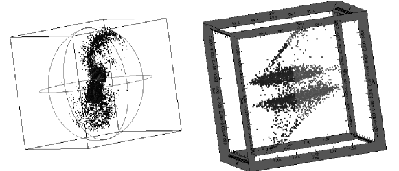
Figure 1.: Mapping from simulation space (left) to spectral cube space (right) using the orientation of a virtual camera to determine the mapping. Data is from an $N$-body simulation of a galaxy merger. The spectral cube has been oriented independently to show velocity-space features.

We are using the S2PLOT 3D-graphics library (Barnes et al. 2006) to develop a framework where models can be examined interactively alongside their spectral-cube projections. This approach enables an increased intuitive understanding of complex kinematical structures. As a simple, yet powerful application development library (C/C++/Fortran), S2PLOT provides customizable user interaction via keyboard and mouse controls; output to mono- and stereoscopic displays; and support for publication in 3D-PDF format (e.g. Barnes & Fluke 2008) via VRML-export with a single key press. Simulation inputs and spectral cube data formats can be handled with custom code or standard C libraries (e.g. cfitiso for FITS files). Figure 2 shows a screenshot from a prototype application – screen elements are described in the caption, and image annotations identify the main S2PLOT functionality we use.

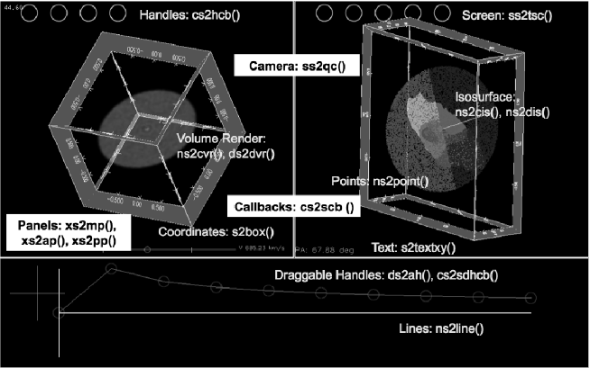
Figure 2.: Screenshot from a prototype S2PLOT application for interactive visualization of model and spectral cube data. The top left panel is model space, the top right panel is spectral cube space, and the bottom panel is an interactive rotation curve. Annotation on the figure gives the main S2PLOT functionality we are using. The model in this example is a rotating disk.

We note our S2PLOT approach is limited by the workstation’s graphics memory, and may not be suitable for very large spectral data cubes ($>512^{3}$ voxels). To this end, we anticipate integrating our approach with a graphics processing unit (GPU) based volume rendering system (see Hassan et al. 2009). Alternatively, it may be sufficient to select sub-volumes to analyze.

We intend to include support for the following basic functionality: generation of standard model components such as rotating disks, warps, hot-spots, expanding shells, $N$-body simulated data; model-specific controls (e.g. interactive rotation curves and density profiles for disk models); realistic noise; overlay of simulated spectral data on observational data; and integrated quantitative analysis tools, such as 3D Cartesian shapelet decomposition.

2. Quantitative Analysis with 3D Cartesian Shapelets

The one- and two-dimensional Cartesian shapelets formalism was introduced by Refregier (2003). In one dimension, shapelets form an orthonormal basis set:

$$\phi_{n}(x) \equiv (2^{n}\pi^{1/2}n!)^{-1/2}H_{n}(x)e^{-x^{2}/2}$$ (4)

$$B_{n}(x;\beta) \equiv \beta^{-1/2}\phi_{n}(\beta^{-1}x)$$ (5)

where $n$ is the shapelet order, $H_{n}(x)$, is the $n$-th Hermite polynomial, and $\beta$ is a scale factor. We have recently extended the Cartesian approach to 3D, deriving a number of important analytic relationships (Fluke et al. in prep). While a full presentation is beyond the scope of this paper, the orthonormality of shapelet states enables us to write 3D shapelets in terms of functions:

$$B_{3,{\mathbf{n}}}({\mathbf{x}};\beta)\equiv\beta^{-3/2}\phi_{n_{1}}(\beta^{-1}x)\phi_{n_{2}}(\beta^{-1}y)\phi_{n_{3}}(\beta^{-1}z),$$ (6)

where ${\mathbf{n}}=(n_{1},n_{2},n_{3})$ are the integer shapelet orders. An arbitrary (sufficiently well-behaved) 3D structure, $f_{3}({\mathbf{x}})$, can be decomposed into a weighted sum of shapelet coeffecients, $f_{3,{\mathbf{n}}}$, by integration over a volume, $V$:

$$f_{3,\mathbf{n}}=\int_{V}f_{3}(\mathbf{x})B_{3,\mathbf{n}}(\mathbf{x};\beta){\rm d}^{3}x$$ (7)

subject to $n_{1}+n_{2}+n_{3}\leq n_{\rm max}$, and an “optimal” $\beta$-value. The shapelet reconstruction is:

$$\hat{f}_{3}(\mathbf{x})=\sum_{n_{1},n_{2},n_{3}}^{n_{\rm max}}\alpha(\mathbf{n})f_{3,\mathbf{n}}B_{3,\mathbf{n}}(\mathbf{x};\beta),$$ (8)

where $\alpha(\mathbf{n})$ is an optional filter term. An example of the decomposition and reconstruction process for a mock spectral data cube (no noise) is shown in Figure 3. As a highly parallel task,

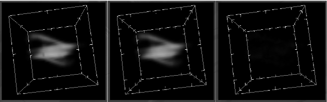
Figure 3.: Shapelet decomposition of a spectral data cube with $57^{3}$ voxels. (Left) input cube; (middle) shapelet reconstruction; (right) residual cube. The basic features of the input cube are well-recovered.

the decomposition and reconstruction processes can be efficiently implemented on a GPU (Barsdell et al. 2009).

3. Conclusion

We are using the S2PLOT programming library to enable interactive, visualization-directed model-fitting of spectral data cubes, leading to improved intuitive understanding of complex kinematic structures. Shapelet space provides new opportunities for quantitative analysis of complex 3D structures. We intend a public code release on completion.

References

Barnes, D. G., Fluke, C. J., Bourke, P. D., & Parry, O. T. 2006, PASA, 23, 82

Barnes, D. G., & Fluke, C. J. 2008, NewA, 13, 599

Barsdell, B. R., Barnes, D. G., & Fluke, C. J. 2009, in ASP Conf. Ser. YYY, ADASS XIX, ed. Y. Mizumoto, K.-I. Morita& M. Ohishi (San Francisco: ASP), [P05]

Begeman, K. G. 1989, A&A, 223, 47

Fluke, C. J., Malec, A., Barsdell, B. R., Lasky, P. D., Beer, C. in prep

Hassan, A. H., Fluke, C. J., Barnes, D. G. 2009, in ASP Conf. Ser. YYY, ADASS XIX, ed. Y. Mizumoto, K.-I. Morita& M. Ohishi (San Francisco: ASP), [P27]

Refregier, A. 2003, MNRAS, 338, 35

Rogstad, D.H., Lockhart, I.A., & Wright, M.C.H. 1974, ApJ, 193, 309