Energy transfer in binary collisions of two gyrating charged particles in a magnetic field

Abstract

Binary collisions of the gyrating charged particles in an external magnetic field are considered within a classical second-order perturbation theory, i.e., up to contributions which are quadratic in the binary interaction, starting from the unperturbed helical motion of the particles. The calculations are done with the help of a binary collisions treatment which is valid for any strength of the magnetic field and involves all harmonics of the particles cyclotron motion. The energy transfer is explicitly calculated for a regularized and screened potential which is both of finite range and nonsingular at the origin. The validity of the perturbation treatment is evaluated by comparing with classical trajectory Monte Carlo (CTMC) calculations which also allow to investigate the strong collisions with large energy and velocity transfer at low velocities. For large initial velocities on the other hand, only small velocity transfers occur. There the nonperturbative numerical CTMC results agree excellently with the predictions of the perturbative treatment.

I Introduction

In the presence of an external magnetic field $\mathbf{B}$ the problem of two charged particles cannot be solved in a closed form as the relative motion and the motion of the center of mass are coupled to each other. Therefore no theory exists for a solution of this problem that is uniformly valid for any strength of the magnetic field and the Coulomb force between the particles. The energy loss of ion beams and the related processes in a magnetized plasmas which are important in many areas of physics such as transport, heating, magnetic confinement of thermonuclear plasmas and astrophysics are examples of physical situations where this problem arises. This topic was studied starting with the classic papers in Ref. ros60, using kinetic equation approach, where the binary collisions of the particles are masked due to the velocity average in the collision operator. Recent applications are the cooling of heavy ion beams by electrons sor83 ; pot90 ; mes94 ; men08 and the energy transfer for heavy-ion inertial confinement fusion.pro08

Calculations have been performed for binary collisions (BC) between magnetized electrons sia76 ; gli92 and for collisions between magnetized electrons and ions.gzwi99 ; zwi00 ; zwi02 ; zwi06 ; toe02 ; ner03 ; ner07 ; ner09 In the presence of a magnetic field only the total energy $E$ of the interacting particles is conserved but not the relative and center of mass energies separately. In addition, the rotational symmetry of the system is broken, and as a consequence only the component of the angular momentum parallel to the magnetic field is a constant of motion. The apparently simple problem of charged particle interaction in a magnetic field is in fact a problem of considerable complexity and the additional degree of freedom of the cyclotron orbital motion produces a chaotic system with two degrees of freedom.gut90 ; sch00 ; bhu02 ; ner07

In this paper we consider the BC between two gyrating charged particles treating the interaction (Coulomb) as a perturbation to their helical motions. For electron-heavy ion collisions this has been done previously in first-order in the ion charge $Z$ for an ion at rest gel97 and up to $Z^{2}$ for an uniformly moving heavy ion. toe02 ; ner03 ; ner07 ; ner09 Here we focus on second-order perturbation theory and its comparison with classical trajectory Monte Carlo (CTMC) simulations. The present work considerably extends the earlier studies in Refs. ner07, ; ner03, ; ner09, where the second-order energy transfer was calculated for an electron-heavy ion BC neglecting the gyration of the ion or assuming identical gyrating particles (e.g. electrons). But in some cases of an interaction of magnetized electrons with light ions (e.g. protons, antiprotons) at a rather strong magnetic field (e.g. in traps) the cyclotron motion of the ion cannot be neglected.

The general expressions for the energy transfers are briefly discussed in Sec. II. In Sec. III we discuss the perturbative methodology used in this work. Then we turn to the explicit calculation of the second-order energy transfer for two arbitrary gyrating particle collision and without any restriction on the magnetic field. In Sec. IV the results of the perturbative BC model are compared with CTMC simulations. The results are summarized and discussed in Sec. V. The small velocity limits of the energy transfers are derived in the Appendix.

II Binary collision formulation

For our description of BC we start with the equations of motion for two charged particles moving in a homogeneous magnetic field and the related conservation laws in general. Next the quantities of interest, the velocity transfer, and the energy transfer of particles during the binary collision will be introduced and discussed, before we turn to the solution of the equations of motion in the subsequent section. For further details we refer to Refs. ner07, ; ner03, ; ner09, .

We consider two point charges with masses $m_{1}$ and $m_{2}$ and charges $q_{1}e$ and $q_{2}e$, respectively, moving in a homogeneous magnetic field $\mathbf{B}=B\mathbf{b}$ and interacting with the potential $q_{1}q_{2}e\!\!\!/^{2}U(\mathbf{r})$ with $e\!\!\!/^{2}=e^{2}/4\pi\varepsilon_{0}$. Here $\varepsilon_{0}$ is the permittivity of the vacuum and $\mathbf{r}=\mathbf{r}_{1}-\mathbf{r}_{2}$ is the relative coordinate of the colliding particles.

In plasma applications the bare Coulomb interaction $U_{\mathrm{C}}(\mathbf{r})=1/r$ is shielded by the surrounding plasma particles and the interaction may be modeled by $U_{\mathrm{D}}(\mathbf{r})=e^{-r/\lambda}/r$. Relative velocities which exceed the thermal velocity lead to an asymmetric interaction potential which in general considerably complicates the theoretical description. It has been shown, however, that such a dynamic, highly asymmetric interaction potential can be replaced with an effective spherically symmetric velocity-dependent interaction $U_{\mathrm{D}}(\mathbf{r})$ with a velocity-dependent screening length $\lambda$.zwi99 ; zwi00 ; gzwi02 We adopt these findings for our present considerations and assume a spherically symmetric interaction with a given fixed screening length in both our analytic expressions and the CTMC simulations. For the envisaged applications of our given results, such as cooling forces, stopping power, etc., which typically involves an average over the velocity distribution, the screening length has then to be replaced by an appropriately chosen velocity-dependent one.

The quantum uncertainty principle prevents particles (for $q_{1}q_{2}<0$) from falling into the center of these potentials. In a classical picture this can be achieved by regularization of $U(\mathbf{r})$ at the origin. Such a regularized potential (pseudopotential) has been derived from quantum statistical considerations.kel63 ; deu77 In our forthcoming investigations we take the functional form of this short distance correction and, including as well the screening contribution, hence use the interaction $U_{\mathrm{R}}(\mathbf{r})=(1-e^{-r/\lambdabar})e^{-r/\lambda}/r$. It should be emphasized, however, that the use of this regularized interaction, where $\lambdabar$ is usually related to the (thermal) de Broglie wavelength,kel63 ; deu77 here essentially represents an alternative implementation of the standard (lower) cutoff procedure needed to handle the hard collisions in a classical perturbative approach where $\lambdabar$ is taken as a given constant or as a function of the classical collision diameter (see Sec. IV).

Introducing the cyclotron frequencies of the particles $\omega_{c\nu}=|q_{\nu}|eB/m_{\nu}$ (with $\nu=1,2$) we start with the classical equations of motion

$${\dot{\mathbf{v}}}_{\nu}(t)-\varsigma_{\nu}\omega_{c\nu}\left[\mathbf{v}_{\nu}(t)\times\mathbf{b}\right]=\varrho_{\nu}\frac{q_{1}q_{2}e\!\!\!/^{2}}{m_{\nu}}\mathbf{F[r}(t)],$$ (1)

where $\varsigma_{\nu}=|q_{\nu}|/q_{\nu}$, $\varrho_{1}=1$, $\varrho_{2}=-1$. Here $q_{1}q_{2}e\!\!\!/^{2}\mathbf{F}[\mathbf{r}(t)]$ $(\mathbf{F}=-\partial U/\partial\mathbf{r})$ is the force exerted by particle 2 on particle 1. In the presence of an external magnetic field, the Lagrangian and the corresponding equations of motion cannot be separated into parts describing the relative motion $[\mathbf{r}=\mathbf{r}_{1}-\mathbf{r}_{2},\mathbf{v}=\dot{\mathbf{r}}]$ and the motion of the cm $[\mathbf{R}=(m_{1}\mathbf{r}_{1}+m_{2}\mathbf{r}_{2})/(m_{1}+m_{2}),\mathbf{V}=\dot{\mathbf{R}}]$, in general.sia76 ; zwi02 ; toe02 ; ner03 ; ner09 ; ner07 Introducing the reduced and the total masses $1/\mu=1/m_{1}+1/m_{2}$, $M=m_{1}+m_{2}$, respectively, and recalling that $\mathbf{v}_{\nu}(t)=\mathbf{V}(t)+\varrho_{\nu}(\mu/m_{\nu})\mathbf{v}(t)$ the equations of the relative and the cm motion are

$${\dot{\mathbf{v}}}-\omega_{3}\left[\mathbf{v}\times\mathbf{b}\right]=\omega_{2}\left[\mathbf{V}\times\mathbf{b}\right]+\frac{q_{1}q_{2}e\!\!\!/^{2}}{\mu}\mathbf{F[r}(t)],$$ (2)

$${\dot{\mathbf{V}}}-\omega_{1}\left[\mathbf{V}\times\mathbf{b}\right]=\frac{\mu}{M}\omega_{2}\left[\mathbf{v}\times\mathbf{b}\right].$$ (3)

The frequencies $\omega_{1}$, $\omega_{2}$ and $\omega_{3}$ are expressed in terms of the cyclotron frequencies of the particles, $\omega_{1}=(m_{1}\varsigma_{1}\omega_{c1}+m_{2}\varsigma_{2}\omega_{c2})/M$, $\omega_{2}=\varsigma_{1}\omega_{c1}-\varsigma_{2}\omega_{c2}$, $\omega_{3}=(m_{2}\varsigma_{1}\omega_{c1}+m_{1}\varsigma_{2}\omega_{c2})/M$. Note that the quantities $|\omega_{1}|$ and $|\omega_{2}|$ play the role of the cm and relative cyclotron frequencies. The coupled, nonlinear differential equations (2) and (3) (or Eq. (1)) completely describe the motion of the particles. For solving the scattering problem, they have to be integrated numerically for a complete set of the initial conditions.

From Eqs. (2) and (3) follow the conservation of the parallel component of the cm velocity ${\mathbf{V}}(t)\cdot\mathbf{b}=V_{0\parallel}$ and the total energy but since, in general, the relative and center-of-mass motions are coupled the relative $E_{\mathrm{r}}$ and cm $E_{\mathrm{cm}}$ energies are not conserved separately. An exception is the case with $\omega_{2}=0$ (or $q_{1}/m_{1}=q_{2}/m_{2}$) where the energies $E_{\mathrm{r}}$ and $E_{\mathrm{cm}}$ are conserved separately.

In the general case the rate $dE_{\nu}/dt$ at which the energy $E_{\nu}=m_{\nu}v_{\nu}^{2}/2$ of particle $\nu$ changes during the collision with the other particle can be obtained by multiplying the equation of motion for particle $\nu$ by its velocity $\mathbf{v}_{\nu}(t)$. The integration of this rate over the whole collision yields the energy transferner03 ; ner07 ; ner09

$$\Delta E_{1}=-iq_{1}q_{2}e\!\!\!/^{2}\int d\mathbf{k}U(\mathbf{k})\int_{-\infty}^{\infty}[\mathbf{k}\cdot\mathbf{V}(t)]e^{i\mathbf{k}\cdot\mathbf{r}(t)}dt$$ (4)

assuming that for $t\to\pm\infty$, $r(t)\to\infty$ and $U[\mathbf{r}(t)]\to 0$. According to the conservation of total energy we have $\Delta E_{2}=-\Delta E_{1}$, as it can be directly seen from Eqs. (1) and (4). In Eq. (4) the force $\mathbf{F}(\mathbf{r})$ has been written using a Fourier transformation in space.

III Perturbative treatment

We now seek an approximate solution of Eqs. (1)-(3) by assuming the interaction force between the particles as a perturbation to their free helical motion. For the case of electron-ion (without cyclotron motion of the ion) and electron-electron scattering the corresponding considerations and derivations are discussed in Refs. ner07, ; ner09, . We therefore focus here on the general case.

We look for a solution of Eq. (1) for the variables $\mathbf{r}_{\nu},\mathbf{v}_{\nu}=\dot{\mathbf{r}}_{\nu}$, or alternatively, of Eqs. (2) and (3)) for the variables $\mathbf{r},\mathbf{v}=\dot{\mathbf{r}}$ and $\mathbf{R},\mathbf{V}=\dot{\mathbf{R}}$, in a perturbative manner ner07 ; ner09 , i.e. $\mathbf{r}_{\nu}=\mathbf{r}_{\nu}^{(0)}+\mathbf{r}_{\nu}^{(1)}+...$ and $\mathbf{R}=\mathbf{R}_{0}+\mathbf{R}_{1}+...$, $\mathbf{r}=\mathbf{r}_{0}+\mathbf{r}^{(1)}+...$ Starting point is the zero–order unperturbed helical motion of two particles in the laboratory frame with $\mathbf{v}_{\nu}^{(0)}(t)=\dot{\mathbf{r}}_{\nu}^{(0)}(t)$ and

$$\mathbf{r}_{\nu}^{(0)}\left(t\right)=\widetilde{\mathbf{R}}_{\nu}+\mathbf{b}v_{0\nu\parallel}t$$ (5)

$$+a_{\nu}\left[\mathbf{u}_{\nu}\sin\left(\omega_{c\nu}t\right)+\varsigma_{\nu}\left[\mathbf{b}\times\mathbf{u}_{\nu}\right]\cos\left(\omega_{c\nu}t\right)\right],$$

where $\mathbf{u}_{\nu}=(\cos\varphi_{\nu},\sin\varphi_{\nu})$ ($\varphi_{\nu}$ is the initial phase of the particle $\nu$) is the unit vector perpendicular to the magnetic field, $v_{0\nu\parallel}$ and $v_{0\nu\bot}\mathbf{u}_{\nu}$ (with $v_{0\nu\bot}\geqslant 0$) are the unperturbed velocity components parallel and perpendicular to $\mathbf{b}$, respectively. Here $a_{\nu}=v_{0\nu\perp}/\omega_{c\nu}$ is the cyclotron radius of the particle $\nu$. It should be noted that in Eq. (5) the variables $\mathbf{u}_{\nu}$ and $\widetilde{\mathbf{R}}_{\nu}$ are independent and are defined by the initial conditions. The unperturbed cm ($\mathbf{R}_{0}(t),\mathbf{V}_{0}(t)=\dot{\mathbf{R}}_{0}(t)$) and relative ($\mathbf{r}_{0}(t),\mathbf{v}_{0}(t)=\dot{\mathbf{r}}_{0}(t)$) coordinates and velocities can be easily found from Eq. (5). In general, the cm and relative coordinates and velocities involve two harmonic oscillations with different frequencies, amplitudes and phases. Therefore in the plane perpendicular to $\mathbf{b}$ these quantities cannot be represented in the form of a simple cyclotron motion with constant amplitudes and phases as in the case of electron-electron (or electron-positron) collisions.ner09

The equation for the first-order velocity correction is given by

$${\dot{\mathbf{v}}}_{\nu}^{(1)}(t)-\varsigma_{\nu}\omega_{c\nu}[\mathbf{v}_{\nu}^{(1)}(t)\times\mathbf{b}]=\varrho_{\nu}\frac{q_{1}q_{2}e\!\!\!/^{2}}{m_{\nu}}\mathbf{F[r}_{0}(t)],$$ (6)

where the solutions can be given by an integral involving the force $\mathbf{F[r}_{0}(t)]$ with $\mathbf{r}_{0}(t)=\mathbf{r}_{1}^{(0)}(t)-\mathbf{r}_{2}^{(0)}(t)$ and the unperturbed trajectory (5) by similar expressions as Eqs. (43)-(46) of Ref. ner03, (see also Ref. ner07, ; ner09, ).

The first- ($\Delta E^{(1)}_{1}$) and the second-order ($\Delta E^{(2)}_{1}$) energy transfers of the particle 1 can be evaluated using general Eq. (4). Here we consider only the energy change $\Delta E^{(2)}_{1}$ since the angular averaged $\Delta E^{(1)}_{1}$ vanishes due to the symmetry reasons.ner03 ; ner07 ; ner09 We obtain

$$\Delta E_{1}^{(2)}=q_{1}q_{2}e\!\!\!/^{2}\int d\mathbf{k}U(\mathbf{k})\int_{-\infty}^{\infty}e^{i\mathbf{k}\cdot\mathbf{r}_{0}(t)}dt$$

$$\times\{[\mathbf{k}\cdot\mathbf{r}^{(1)}(t)][\mathbf{k}\cdot\mathbf{V}_{0}(t)]-i[\mathbf{k}\cdot\mathbf{V}_{1}(t)]\}.$$ (7)

Let us recall that here $\mathbf{r}^{(1)}(t)$ and $\mathbf{V}_{1}(t)$ are the first-order relative coordinate and the cm velocity corrections, respectively.

We now introduce the variable $\mathbf{s}=\mathbf{R}_{r\bot}$ which is the component of $\mathbf{R}_{r}=\widetilde{\mathbf{R}}_{1}-\widetilde{\mathbf{R}}_{2}$ perpendicular to the relative velocity of the guiding centers of two particles $v_{r\parallel}\mathbf{b}$, where $v_{r\parallel}=v_{01\parallel}-v_{02\parallel}$. From Eq. (5) we can see that $\mathbf{s}$ is the distance of closest approach for the guiding centers of the two particles’ helical motion. For practical applications the energy change is given by the average of $\Delta E_{1}$ with respect to the initial phases of the particles $\varphi_{1}$ and $\varphi_{2}$ and the azimuthal angle $\vartheta_{\mathbf{s}}$ of $\mathbf{s}$. This averaged quantity is denoted by $\langle\Delta E_{1}\rangle$ in the forthcoming considerations.

To evaluate the second-order energy transfer $\Delta E_{1}^{(2)}$ we have to insert Eq. (5) and the solution of Eq. (6) into Eq. (7). This quantity is then averaged with respect to the initial phases of the particles $\varphi_{1}$ and $\varphi_{2}$ and the azimuthal angle $\vartheta_{\mathbf{s}}$ of the impact parameter $\mathbf{s}$. The obtained angular integrals are evaluated using the Fourier series of the exponential function. After averaging the energy transfer $\Delta E_{1}^{(2)}$ with respect to $\varphi_{1}$ and $\varphi_{2}$ the remaining part will depend on $\delta(k_{\parallel}+k_{\parallel}^{\prime})$, i.e. the component of $\mathbf{k}+\mathbf{k}^{\prime}$ along the magnetic field $\mathbf{b}$. This $\delta$-function enforces $\mathbf{k}+\mathbf{k}^{\prime}$ to lie in the plane transverse to $\mathbf{b}$ so that $e^{i(\mathbf{k+k}^{\prime})\cdot\mathbf{R}_{r}}\delta(k_{\parallel}+k_{\parallel}^{\prime})=e^{i\mathbf{Q}\cdot\mathbf{s}}\delta(k_{\parallel}+k_{\parallel}^{\prime})$, where $\mathbf{Q}=\mathbf{k}_{\bot}+\mathbf{k}_{\bot}^{\prime}$. The result of the angular averaging finally reads

$$\langle\Delta E_{1}^{(2)}\rangle=\frac{\pi iq_{1}^{2}q_{2}^{2}e\!\!\!/^{4}}{\mu\left|v_{r\parallel}\right|}\int d\mathbf{k}d\mathbf{k}^{\prime}U\left(\mathbf{k}\right)U\left(\mathbf{k}^{\prime}\right)J_{0}\left(Qs\right)$$

$$\times\delta(k_{\parallel}^{\prime}+k_{\parallel})\sum_{n,m=-\infty}^{\infty}\left(-1\right)^{m+n}e^{i(\theta-\theta^{\prime})(n\varsigma_{1}+m\varsigma_{2})}$$

$$\times\left(k_{\parallel}V_{0\parallel}+\frac{\mu}{m_{2}}n\omega_{c1}-\frac{\mu}{m_{1}}m\omega_{c2}\right)\Bigg{\{}\frac{2k_{\parallel}^{2}H_{n,m}(k_{\perp},k_{\perp}^{\prime})}{\left(\zeta_{n,m}-i0\right)^{2}}$$

$$-\frac{k_{\perp}^{\prime}k_{\perp}}{\zeta_{n,m}-i0}\bigg{[}2iAH_{n,m}(k_{\perp},k_{\perp}^{\prime})\sin(\theta-\theta^{\prime})$$

$$+\frac{\mu}{m_{1}\omega_{c1}}\mathcal{H}_{n,m}(k_{\perp},k_{\perp}^{\prime})+\frac{\mu}{m_{2}\omega_{c2}}\mathcal{P}_{n,m}(k_{\perp},k_{\perp}^{\prime})\bigg{]}\Bigg{\}}.$$ (8)

Here $H_{n,m}=J_{n}(k_{\perp}a_{1})J_{n}(k_{\perp}^{\prime}a_{1})J_{m}(k_{\perp}a_{2})J_{m}(k_{\perp}^{\prime}a_{2})$ and $\mathcal{H}_{n,m}=H_{n-1,m}-H_{n+1,m}$, $\mathcal{P}_{n,m}=H_{n,m-1}-H_{n,m+1}$, $A=\mu\varsigma_{1}/m_{1}\omega_{c1}+\mu\varsigma_{2}/m_{2}\omega_{c2}$, where $J_{n}$ are the Bessel functions of the $n$th order. Also $\zeta_{n,m}=n\omega_{c1}+m\omega_{c2}+k_{\parallel}v_{r\parallel}$, $k_{\parallel}=\mathbf{k}\cdot\mathbf{b}$ and $\mathbf{k}_{\bot}$ are the components of $\mathbf{k}$ parallel and transverse to $\mathbf{b}$, respectively, $\tan\theta=k_{y}/k_{x}$. The series representation (8) of the second-order energy transfer is valid for any strength of the magnetic field.

For most applications it is also useful to integrate the averaged energy transfer, $\langle\Delta E_{1}^{(2)}\rangle$, with respect to the impact parameters $s$ in the full two-dimensional (2D) space. We thus introduce an energy loss cross section (ELCS) gzwi99 ; zwi00 ; ner03 ; ner07 ; ner09 through the relation

$$\sigma=\int_{0}^{\infty}\langle\Delta E_{1}^{(2)}\rangle sds.$$ (9)

As $\sigma$ results from the $s$-integration of the energy transfer (8) one obtains an expression for $\sigma$ which represents an infinite sum over Bessel functions. Moreover, assuming regularized interaction and performing $\mathbf{k}$ integration in $\sigma$ yields an infinite sum over modified Bessel functions (see, e.g., an example for ion-electron collision in Ref. ner07, ). For arbitrary axially symmetric interaction potential similar expression is derived in the Appendix [see Eq. (35)]. However, for practical applications it is much more convenient to use an equivalent integral representation of the ELCS which does not involve any special function. This expression can be derived from the Bessel-function representation of $\sigma$ using the integral representation of the Dirac $\delta$ function as well as the summation formula for $\sum_{n}e^{in\varphi}J_{n}^{2}(a)$.gra80 The energy transfer $\sigma$ after lengthy but straightforward calculations then reads

$$\sigma=\int_{0}^{2\pi}\frac{d\varphi}{2\pi}\overline{\sigma}\left(\varphi\right),\quad\overline{\sigma}(\varphi)=\overline{\sigma}_{\parallel}(\varphi)+\overline{\sigma}_{\bot}(\varphi),$$ (10)

with

$$\overline{\sigma}_{\parallel}\left(\varphi\right)=-\frac{\left(2\pi\right)^{2}q_{1}^{2}q_{2}^{2}e\!\!\!/^{4}\lambda^{2}V_{0\parallel}}{\mu v_{r\parallel}^{3}}\int_{0}^{\infty}tdt\int d\mathbf{k}\left|U\left(\mathbf{k}\right)\right|^{2}$$

$$\times[k_{\parallel}^{2}+k_{\perp}^{2}\phi\left(t\right)]k_{\parallel}\sin\left(k_{\parallel}\lambda t\right)J_{0}\left[2k_{\perp}\mathcal{R}\left(t\right)\right],$$ (11)

$$\overline{\sigma}_{\perp}\left(\varphi\right)=-\frac{\left(2\pi\right)^{2}q_{1}^{2}q_{2}^{2}e\!\!\!/^{4}\lambda}{m_{1}m_{2}v_{r\parallel}^{4}}\int_{0}^{\infty}t^{2}dt\int d\mathbf{k}\left|U\left(\mathbf{k}\right)\right|^{2}k_{\perp}^{2}$$

$$\times\cos\left(k_{\parallel}\lambda t\right)\bigg{\{}\lambda^{2}G_{1}\left(t\right)[k_{\parallel}^{2}+k_{\perp}^{2}\phi\left(t\right)]\frac{J_{1}\left[2k_{\perp}\mathcal{R}\left(t\right)\right]}{2k_{\perp}\mathcal{R}\left(t\right)}$$

$$+G_{2}\left(t\right)J_{0}\left[2k_{\perp}\mathcal{R}\left(t\right)\right]\bigg{\}},$$ (12)

where $\delta_{\nu}=|v_{r\parallel}|/\omega_{c\nu}$ are the relative pitches of the particles helices, divided by $2\pi$ and $\eta_{\nu}=\lambda/\delta_{\nu}=\omega_{c\nu}\lambda/|v_{r\parallel}|$. In Eqs. (11) and (12) the time $t$ is scaled in units $\lambda/|v_{r\parallel}|$, where the length $\lambda$ is specified in the next section. In addition in Eq. (10) the energy transfer $\overline{\sigma}(\varphi)$ has been split into two parts which correspond to the cm motion along [$\overline{\sigma}_{\parallel}(\varphi)$] and transverse [$\overline{\sigma}_{\perp}(\varphi)$] to the magnetic field, where $\varphi=\varphi_{1}-\varphi_{2}$ is the difference of the initial phases of the particles. Also

$$\phi\left(t\right)=\frac{\mu}{m_{1}}\frac{\sin\left(\eta_{1}t\right)}{\eta_{1}t}+\frac{\mu}{m_{2}}\frac{\sin\left(\eta_{2}t\right)}{\eta_{2}t},$$ (13)

$$\mathcal{R}^{2}\left(t\right)=a_{1}^{2}\sin^{2}\frac{\eta_{1}t}{2}+a_{2}^{2}\sin^{2}\frac{\eta_{2}t}{2}$$

$$-2a_{1}a_{2}\sin\frac{\eta_{1}t}{2}\sin\frac{\eta_{2}t}{2}\cos\varphi,$$ (14)

$$G_{1}\left(t\right)=m_{1}v_{01\perp}^{2}\frac{\sin\left(\eta_{1}t\right)}{\eta_{1}t}-m_{2}v_{02\perp}^{2}\frac{\sin\left(\eta_{2}t\right)}{\eta_{2}t}+2v_{01\perp}v_{02\perp}$$

$$\times\cos\varphi\left(m_{2}\frac{\sin\frac{\eta_{1}t}{2}}{\eta_{1}t}\cos\frac{\eta_{2}t}{2}-m_{1}\frac{\sin\frac{\eta_{2}t}{2}}{\eta_{2}t}\cos\frac{\eta_{1}t}{2}\right),$$ (15)

$$G_{2}\left(t\right)=\mu v_{r\parallel}^{2}\frac{\cos\left(\eta_{2}t\right)-\cos\left(\eta_{1}t\right)}{t^{2}}.$$ (16)

Here the quantity $\mathcal{R}(t)$ represents an effective relative cyclotron radius of the two particles. The second term in Eq. (12) proportional to the function $G_{2}(t)$ is the contribution of the cm velocity perturbation, see the second term of Eq. (7). This perturbation and hence this corresponding term was absent in our previous considerations for electron-electron and electron-ion collisions.

An expression similar to Eq. (8) (or Eqs. (10)-(12)) has been obtained for electron-electron collisionner09 and for electron-heavy ion (without cyclotron motion of the ion) collision.ner03 ; ner07 ; ner09 In contrast to these specific cases Eqs. (8) and (10)-(12) are valid for the collision of two arbitrary charged particles. The results obtained in Refs. ner03, ; ner07, ; ner09, can be easily derived from these general expressions. The electron-electron case is recovered assuming that $m_{1}=m_{2}=m$, $q_{1}=q_{2}=q$, i.e., $\omega_{c1}=\omega_{c2}=\omega_{c}$, $\eta_{1}=\eta_{2}=\eta$, $\mu=m/2$. Then the term proportional to the function $G_{2}(t)$ in Eq. (12) vanishes and the remaining expressions coincide with the results of Ref. ner09, . It should be noted that for identical particles (e.g. electrons) the effective cyclotron radius is given by $\mathcal{R}(t)=a\sin(\eta t/2)$, where $a^{2}=a_{1}^{2}+a_{2}^{2}-2a_{1}a_{2}\cos\varphi$ is the cyclotron radius of the particles in the relative frame.ner09 For electron-heavy ion collision we assume that the ion mass tends to infinity, $m_{2}\to\infty$, and $v_{02\perp}=0$ (ion moves along the magnetic field direction). Therefore $\mu\to m_{1}=m$, $\omega_{c2}\to 0$ ($\eta_{2}\to 0$). In this case the transverse ELCS vanishes and the longitudinal cross section coincides with the results of Ref. ner09, .

Next we also consider the ELCS $\overline{\sigma}_{\parallel}(\varphi)$ and $\overline{\sigma}_{\bot}(\varphi)$ for vanishing cyclotron radii, $a_{1},a_{2}\to 0$, i.e. when initially the particles move along the magnetic field ($v_{01\bot}=v_{02\bot}=0$). In this limit $\overline{\sigma}_{\bot}(\varphi)\neq 0$ as in the cases of two identical particles collision or ion-electron collision. For any axially symmetric interaction potential, $U(\mathbf{k})=U(|k_{\parallel}|,k_{\perp})$, the straightforward integration in Eqs. (11) and (12) yields

$$\overline{\sigma}_{\parallel}\left(\varphi\right)=-\frac{2q_{1}^{2}q_{2}^{2}e\!\!\!/^{4}V_{0\parallel}}{v_{r\parallel}^{3}}\left[\frac{\mathcal{F}_{0}\left(\delta_{1}^{-1}\right)}{m_{1}}+\frac{\mathcal{F}_{0}\left(\delta_{2}^{-1}\right)}{m_{2}}\right],$$ (17)

$$\overline{\sigma}_{\perp}\left(\varphi\right)=\frac{2q_{1}^{2}q_{2}^{2}e\!\!\!/^{4}}{Mv_{r\parallel}^{2}}\left[\mathcal{F}_{0}\left(\delta_{1}^{-1}\right)-\mathcal{F}_{0}\left(\delta_{2}^{-1}\right)\right],$$ (18)

where

$$\mathcal{F}_{0}\left(\kappa\right)=\frac{\left(2\pi\right)^{4}}{4}\int_{0}^{\infty}U^{2}\left(\kappa,k_{\perp}\right)k_{\perp}^{3}dk_{\perp}.$$ (19)

The averaged energy transfer, Eq. (8), can be evaluated without further approximation for any axially symmetric interaction potential. In this case the energy transfer can be represented as the sum of all cyclotron harmonics as it has been done for ion-electron interaction in Ref. ner07, and for electron-electron interaction in Ref. ner09, .

In the following we consider the regularized screened potential introduced in Sec. II with

$$U_{\mathrm{R}}(k_{\parallel},k_{\perp})=\frac{2}{(2\pi)^{2}}\left(\frac{1}{k_{\perp}^{2}+\kappa^{2}}-\frac{1}{k_{\perp}^{2}+\chi^{2}}\right),$$ (20)

where $\kappa^{2}=k_{\parallel}^{2}+\lambda^{-2}$, $\chi^{2}=k_{\parallel}^{2}+d^{-2}$, $d^{-1}=\lambda^{-1}+\lambdabar^{-1}$.

As we discussed above the energy transfer (8) must be integrated with respect to the impact parameters $s$ for practical applications. For general interaction potential this is given by Eqs. (9)-(12). In general for a study of the convergence of the $s$-integrated energy transfers we note that the case with some value $s=s_{c}$ is most critical for the convergence of the ELCS. This is intuitively clear as the gyrating particles at $|a_{1}-a_{2}|<s<a_{1}+a_{2}$ may hit each other on such a trajectory (see Ref. ner07, for some explicit examples). This should not matter for the potential (20), which has been regularized near the origin for exactly that purpose.

For the present case of the regularized interaction potential, substituting Eq. (20) into Eqs. (11) and (12), we obtain

$$\overline{\sigma}_{\parallel}(\varphi)=-\frac{q_{1}^{2}q_{2}^{2}e\!\!\!/^{4}V_{0\parallel}}{\mu v_{r\parallel}^{3}}\int_{0}^{\infty}\frac{t^{2}dt}{R^{3}(t)}\bigg{\{}e^{-R(t)}\bigg{[}\mathcal{F}_{1}[R(t),t,t]$$

$$+\frac{4}{\varkappa^{2}-1}\mathcal{F}_{2}[R(t),t,t]\bigg{]}+e^{-\varkappa R(t)}\bigg{[}\mathcal{F}_{1}[\varkappa R(t),\varkappa t,t]$$

$$-\frac{4\varkappa^{2}}{\varkappa^{2}-1}\mathcal{F}_{2}[\varkappa R(t),\varkappa t,t]\bigg{]}\bigg{\}},$$ (21)

$$\overline{\sigma}_{\perp}(\varphi)=-\frac{q_{1}^{2}q_{2}^{2}e\!\!\!/^{4}}{m_{1}m_{2}v_{r\parallel}^{4}}\int_{0}^{\infty}\frac{t^{2}dt}{R^{3}(t)}\Bigg{\{}G_{1}(t)\bigg{\{}e^{-R(t)}$$

$$\times\left[\mathcal{F}_{3}[R(t),t,t]+\frac{4}{\varkappa^{2}-1}\mathcal{F}_{4}[R(t),t,t]\right]+e^{-\varkappa R(t)}$$

$$\times\left[\mathcal{F}_{3}[\varkappa R(t),\varkappa t,t]-\frac{4\varkappa^{2}}{\varkappa^{2}-1}\mathcal{F}_{4}[\varkappa R(t),\varkappa t,t]\right]\bigg{\}}$$

$$+G_{2}(t)\bigg{\{}e^{-R(t)}\left[\mathcal{F}_{5}[R(t),t]+\frac{4}{\varkappa^{2}-1}\mathcal{F}_{6}[R(t),t]\right]$$ (22)

$$+\frac{e^{-\varkappa R(t)}}{\varkappa^{2}}\left[\mathcal{F}_{5}[\varkappa R(t),\varkappa t]-\frac{4\varkappa^{2}}{\varkappa^{2}-1}\mathcal{F}_{6}[\varkappa R(t),\varkappa t]\right]\bigg{\}}\Bigg{\}}.$$

Here $R^{2}(t)=t^{2}+(4/\lambda^{2})\mathcal{R}^{2}(t)$, $\varkappa=\lambda/d=1+\lambda/\lambdabar$, and

$$\mathcal{F}_{1}(R,\zeta,t)=2+2R-R^{2}+[1-\phi(t)]\bigg{[}R^{2}+R+1$$

$$-\frac{\zeta^{2}}{R^{2}}(R^{2}+3R+3)\bigg{]},$$ (23)

$$\mathcal{F}_{2}(R,\zeta,t)=R+1-\frac{1}{R^{2}}[1-\phi(t)]\bigg{[}R^{3}+4R^{2}+9R+9$$

$$-\frac{\zeta^{2}}{R^{2}}(R^{3}+6R^{2}+15R+15)\bigg{]},$$ (24)

$$\mathcal{F}_{3}(R,\zeta,t)=2+2R-R^{2}+[1-\phi(t)]\bigg{[}R^{2}-R-1$$

$$-\frac{\zeta^{2}}{R^{2}}(R^{2}+3R+3)\bigg{]},$$ (25)

$$\mathcal{F}_{4}(R,\zeta,t)=R+1-\frac{1}{R^{2}}[1-\phi(t)]\bigg{[}R^{3}+2R^{2}+3R+3$$

$$-\frac{\zeta^{2}}{R^{2}}(R^{3}+6R^{2}+15R+15)\bigg{]},$$ (26)

$$\mathcal{F}_{5}(R,\zeta)=R^{2}\left[1-R+\frac{\zeta^{2}}{R^{2}}(R+1)\right],$$ (27)

$$\mathcal{F}_{6}(R,\zeta)=R^{2}+R+1-\frac{\zeta^{2}}{R^{2}}(R^{2}+3R+3).$$ (28)

Next we consider the ELCS $\overline{\sigma}_{\parallel}(\varphi)$ and $\overline{\sigma}_{\perp}(\varphi)$ for vanishing cyclotron radius, $a_{1},a_{2}\to 0$, i.e. when initially the particles move along the magnetic field ($v_{01\bot}=v_{02\bot}=0$) which are given by Eqs. (17)-(19). Substitution of Eq. (20) into Eq. (19) yields

$$\mathcal{F}_{0}\left(\kappa\right)=\frac{2\kappa^{2}\lambda^{2}+\varkappa^{2}+1}{2\left(\varkappa^{2}-1\right)}\ln\frac{\kappa^{2}\lambda^{2}+\varkappa^{2}}{\kappa^{2}\lambda^{2}+1}-1.$$ (29)

Thus the ELCS at $a_{1},a_{2}\to 0$ are then given by Eqs. (17) and (18), where the function $\mathcal{F}_{0}(\kappa)$ is defined by Eq. (29).

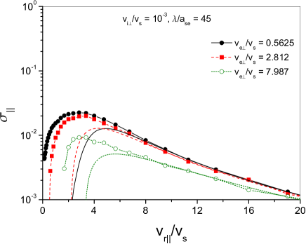
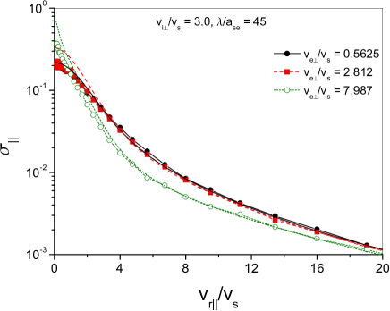
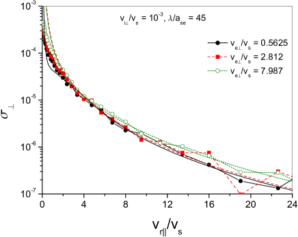
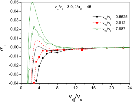
Figure 1: (Color online) Top panels, the ELCS $\sigma_{\parallel}$ for electron–ion ($Z=6$ and $m_{2}/m_{1}\simeq 2.2\times 10^{4}$) collision at $v_{i\bot}/v_{s}=10^{-3}$ (left panel) and $v_{i\bot}/v_{s}=3.0$ (right panel). The curves with and without symbols correspond to CTMC simulations and the second-order perturbative treatment, respectively. Also $\lambda/a_{se}=45$, $v_{e\bot}/v_{s}=0.5625$ (solid lines), $v_{e\bot}/v_{s}=2.812$ (dashed lines), $v_{e\bot}/v_{s}=7.987$ (dotted lines). Bottom panels, same as in top but for $\sigma_{\bot}$.

Equations (17) and (18) with Eq. (29) are approximately valid also for finite cyclotron radii $a_{1}$ and $a_{2}$, assuming that the longitudinal velocity $v_{r\parallel}$ is larger than the transversal ones, $v_{01\perp}$ and $v_{02\perp}$. Indeed, in this case $R(t)\simeq t$ since $\delta_{1},\delta_{2}\gg a_{1},a_{2}$ and in Eqs. (21) and (22) the transversal ELCS $\overline{\sigma}_{\bot}(\varphi)$ can be neglected compared to the longitudinal one. This indicates that in the high velocity limit with $v_{r\parallel}\gg v_{01\perp},$ $v_{02\perp}$ the transversal motion of the particles as well as its cm transversal motion are not important and can be neglected. Since only the contribution of small $t$ is important the function $R(t)$ is approximated by $R(t)\simeq t$. Using this result for $R(t)$ from Eq. (22) and Eqs. (17) and (18) with (29) in the high velocity limit we obtain within the leading term approximation for the ELCS

$$\overline{\sigma}_{\parallel}(\varphi)\simeq-\frac{2q_{1}^{2}q_{2}^{2}e\!\!\!/^{4}V_{0\parallel}}{\mu v_{r\parallel}^{3}}\Lambda(\varkappa),$$ (30)

$$\overline{\sigma}_{\perp}(\varphi)\simeq-\frac{2q_{1}^{2}q_{2}^{2}e\!\!\!/^{4}}{Mv_{r\parallel}^{4}}\left[Q_{1}\Lambda(\varkappa)+Q_{2}\Lambda_{1}(\varkappa)\right],$$ (31)

where $Q_{2}=(\lambda^{2}/2)(\omega_{c1}^{2}-\omega_{c2}^{2})$, $Q_{1}=(m_{1}/\mu)v_{01\perp}^{2}-(m_{2}/\mu)v_{02\perp}^{2}+((m_{2}-m_{1})/\mu)v_{01\perp}v_{02\perp}\cos\varphi$,

$$\Lambda(u)=\frac{u^{2}+1}{u^{2}-1}\ln u-1,$$ (32)

$$\Lambda_{1}\left(u\right)=1+\frac{1}{u^{2}}-\frac{4}{u^{2}-1}\ln u.$$ (33)

Note that $\overline{\sigma}_{\parallel}(\varphi)$ is isotropic, i.e., do not depend on $\varphi$ while $\overline{\sigma}_{\perp}(\varphi)$ contains a term which is proportional to $\cos\varphi$. Also, in the high velocity limit the parallel ELCS, $\overline{\sigma}_{\parallel}(\varphi)$, does not depend on the magnetic field strength. The ELCS decay as $\overline{\sigma}_{\parallel}(\varphi)\sim v_{r\parallel}^{-3}$ and $\overline{\sigma}_{\bot}(\varphi)\sim v_{r\parallel}^{-4}$.

Finally we briefly turn to the case of small relative velocity, $v_{r\parallel}\ll v_{01\bot},v_{02\bot}$. It should be emphasized that Eqs. (21) and (22), are not adopted for evaluation of the ELCS at small velocities. For this purpose it is convenient to use an alternative Bessel-function representation of the ELCS as shown in the Appendix. In addition, it is expected that the limit of small $v_{r\parallel}$ is the most critical regime for a violation of the perturbation theory employed here. Therefore explicit analytical expressions in this limit can be useful for an improvement of the perturbation theory by comparing the analytical results with numerical simulations, see Sec. IV.

IV Results. Comparison with simulations

A fully numerical treatment is required for applications beyond the perturbative regime and for checking the validity of the perturbative approach outlined above. In the present case of binary collisions of two arbitrary particles in a magnetic field and with the effective interaction $U_{\mathrm{R}}(r)$ (20) the numerical evaluation of the BC energy loss is very complicated, but can be successfully investigated by classical trajectory Monte Carlo (CTMC) simulations.gzwi99 ; zwi00 ; zwi02 In the CTMC method abr66 the trajectories for the relative motion between the particles are calculated by a numerical integration of the equations of motion (2) and (3), starting with initial conditions for the parallel ${v}_{r\parallel}$ and the transverse $\mathbf{v}_{0\perp}=\mathbf{v}_{01\perp}-\mathbf{v}_{02\perp}$ relative velocity. The required accuracy is achieved by using a modified velocity-Verlet algorithm which has been specifically designed for particle propagation in a (strong) magnetic field,spr99 ; zwi08 and by adapting continuously the actual time-step by monitoring the constant of motion $E=E_{1}+E_{2}=E_{\mathrm{r}}+E_{\mathrm{cm}}$. The resulting relative deviations of $E$ are of the order of $10^{-6}-10^{-5}$.

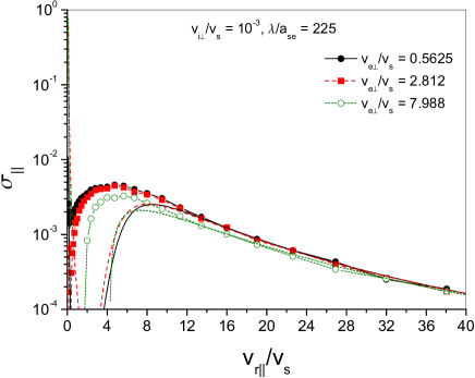
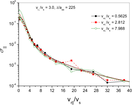
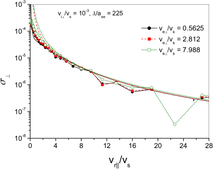
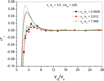
Figure 2: (Color online) Same as in Fig. 1 but for $\lambda/a_{se}=225$ and $v_{e\bot}/v_{s}=7.988$ (dotted lines).

The desired average over the initial phases and the impact parameter $\mathbf{s}$ is performed by a Monte Carlo sampling bin97 ; fis99 of a large number of trajectories with different initial values. The actual number of computed trajectories (typically $10^{5}-10^{6}$ trajectories) is adjusted by monitoring the convergence of the averaging procedure. For further details we refer to Refs. ner07, ; ner09, .

For the forthcoming discussion we put the equation of the relative motion of two particles in a more appropriate dimensionless form by scaling lengths in units of the screening length $\lambda$ and velocities in units of a characteristic velocity $v_{s}$ defined by $v_{s}^{2}=|q_{1}q_{2}|e\!\!\!/^{2}/\mu\lambda$. This velocity gives a measure for the strength of the Coulomb interaction with respect to the (initial) kinetic energy of relative motion $\mu v_{r}^{2}/2$. For $v_{r}<v_{s}$ the kinetic energy is small compared to the characteristic potential energy $|q_{1}q_{2}|e\!\!\!/^{2}/\lambda$ in a screened Coulomb potential and we expect to be in a nonperturbative regime. A perturbative treatment on the other hand should be applicable for $v_{r}\gg v_{s}$.

The scaled version of Eqs. (1)-(3) depends on the four dimensionless parameters $a_{s1}/\lambda$, $a_{s2}/\lambda$, $m_{2}/m_{1}$ and $\lambdabar/\lambda$, and the initial conditions with positions scaled in $\lambda$ and velocities in $v_{s}$. Here $a_{s1}=v_{s}/\omega_{c1}$ and $a_{s2}=v_{s}/\omega_{c2}$ are the cyclotron radii for $v_{1\perp}=v_{2\perp}=v_{s}$ and the parameters $a_{s1}/\lambda\propto a_{s2}/\lambda\propto v_{s}/B$ represents a measure for the strength of the magnetic field compared to the strength of the Coulomb interaction [which is $\propto v_{s}^{2}$]. The ratio $\lambdabar/\lambda$ describes the amount of softening of the screened interaction at $r\to 0$ with $q_{1}q_{2}e\!\!\!/^{2}U_{\mathrm{R}}(r\to 0)\to{q_{1}q_{2}e\!\!\!/^{2}}/\lambdabar$.

In the analytical perturbative approach we thus apply the same scaling of length and velocities and introduce for two particles collisions the dimensionless ELCS

$$\sigma_{\alpha}=-\frac{1}{\mu v_{s}\mathcal{V}_{\alpha}\lambda^{2}}\int_{0}^{2\pi}\frac{d\varphi}{2\pi}\overline{\sigma}_{\alpha}\left(\varphi\right),$$ (34)

where $\alpha=\parallel,\bot$, $\mathcal{V}_{\parallel}=V_{0\parallel}$ and $\mathcal{V}_{\bot}=v_{s}$.

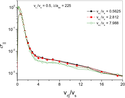
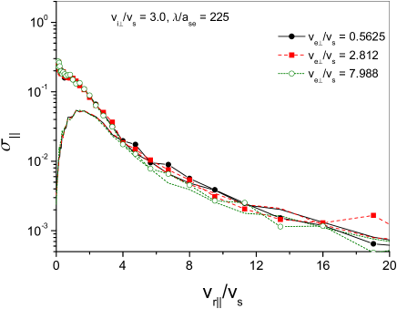
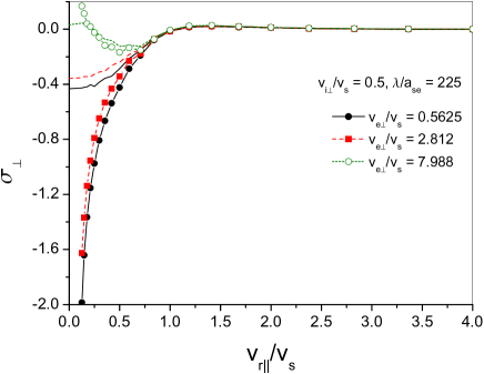
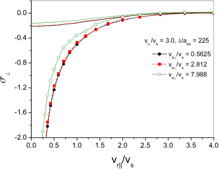
Figure 3: (Color online) Top panels, the ELCS $\sigma_{\parallel}$ for electron-ion ($Z=6$ and $m_{2}/m_{1}\simeq 2.2\times 10^{4}$) collision at $v_{i\bot}/v_{s}=0.5$ (left panel) and $v_{i\bot}/v_{s}=3.0$ (right panel). The curves with and without symbols correspond to the CTMC simulations with and without ion gyration effects, respectively. Also $\lambda/a_{se}=225$, $v_{e\bot}/v_{s}=0.5625$ (solid lines), $v_{e\bot}/v_{s}=2.812$ (dashed lines) and $v_{e\bot}/v_{s}=7.988$ (dotted lines). Bottom panels, same as in top but for $\sigma_{\bot}$.

Next we specify the cutoff parameter $\lambdabar$ which is a measure of softening of the interaction potential at short distances. As we discussed in previous section the regularization in the potential (20) is sufficient to guarantee the existence of the $s$-integrated energy transfers, but there remains the problem of treating hard collisions. For a perturbation treatment the change in relative velocity must be small compared to $v_{r}$ and this condition is increasingly difficult to fulfill in the regime $v_{r}\to 0$. This suggests a physically reasonable procedure: the potential must be softened near the origin. In fact the parameter $\lambdabar$ should be related to the de Broglie wavelength which is inversely proportional to $v_{r}$. Here within classical picture we employ in a perturbative treatment the dynamical cutoff parameter $\varkappa(v_{r\parallel})=1+\lambda/\lambdabar(v_{r\parallel})$,ner09 where $\lambdabar^{2}(v_{r\parallel})=Cb^{2}_{0}(v_{r\parallel})+\lambdabar^{2}_{0}$ with $b_{0}(v_{r\parallel})=\lambda v^{2}_{s}/(v^{2}_{r\parallel}+v^{2}_{0})$, $v^{2}_{0}=v^{2}_{01\perp}+v^{2}_{02\perp}$. Here $\lambdabar_{0}$ is some constant cutoff parameter, and $b_{0}(v_{r\parallel})$ is the distance of closest approach of two charged particles in the absence of a magnetic field. Also in $\lambdabar(v_{r\parallel})$ we have introduced a fitting parameter $C\simeq 0.292$. In Ref. ner09, this parameter is deduced from the comparison of the ELCS (9) with an exact asymptotic expression derived in Ref. hah71, for the Yukawa-type (i.e., with $\lambdabar\to 0$) interaction potential. As has been shown in Ref. ner09, the second-order ELCS for electron-electron and electron-ion (but wihtout gyration of the ion) collisions with dynamical cutoff parameter $\lambdabar(v_{r\parallel})$ excellently agrees with CTMC simulations at high velocities. The CTMC simulations have been carried out with constant $\lambdabar=\lambdabar_{0}\ll\lambda$, that is, the interaction is almost Coulomb at short distances.

The ELCS are presented in Figs. 1-4. These results are obtained for the BC of an electron (particle 1, $q_{1}=-1$) with an ion (particle 2, $q_{2}=Z$) in a strong magnetic field. Shown are $\sigma_{\parallel}$ and $\sigma_{\perp}$ as functions of $v_{r\parallel}/v_{s}$ for fixed transverse velocity of the ion $v_{02\bot}=v_{i\bot}$ and the strength of the magnetic field $\lambda/a_{se}=B/B_{s}$ (with $a_{se}=a_{s1}$, $B_{s}=m_{1}v_{s}/e\lambda$) and varying the transversal velocity of the electron $v_{01\bot}=v_{e\bot}$. For each triplet of fixed $v_{i\bot}$, $v_{e\bot}$ and $B$ the cyclotron radii $a_{1}$, $a_{2}$ and $a_{s2}=a_{si}$ can be easily determined. Both the CTMC and second-order calculations have been done for a regularized potential $U_{\mathrm{R}}$ with $\nu_{0}=\lambdabar_{0}/\lambda=10^{-4}$. Note that in all cases shown in Figs. 1-4 we have $a_{se}/\lambda\ll 1$ and the ELCS is not sensitive to this parameter when $a_{se}/\lambda\to 0$ (see, e.g., Fig. 4).

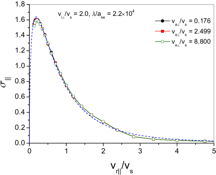
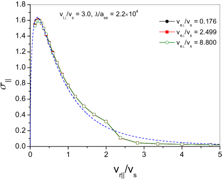
Figure 4: (Color online) The ELCS $\sigma_{\parallel}$ for electron–antiproton ($Z=-1$ and $m_{2}/m_{1}=1836$) collision at $v_{i\bot}/v_{s}=2.0$ (left panel) and $v_{i\bot}/v_{s}=3.0$ (right panel). The curves with symbols correspond to CTMC simulations. Also $\lambda/a_{se}=2.2\times 10^{4}$, $v_{e\bot}/v_{s}=0.176$ (filled circles), $v_{e\bot}/v_{s}=2.499$ (squares), $v_{e\bot}/v_{s}=8.8$ (open circles). The dashed curves are obtained employing a model suggested in Ref. ner09, .

Comparisons of the ELCS determined by the CTMC simulations and the second-order perturbative treatment Eqs. (21), (22), and (34) are presented in Figs. 1 and 2. It is clearly observed that in the regimes of large relative velocities the second order perturbative treatment agrees almost perfectly (i.e. within the unavoidable numerical fluctuations) with the CTMC results. In addition in the limit of very large velocities $v_{r\parallel}/v_{s}\gg 1$ the ELCS $\sigma_{\parallel}$ calculated either within perturbation theory or CTMC method with different strength of the magnetic field and $v_{i\perp},v_{e\perp}$ converge to the same value. This behavior agrees with the predictions of the asymptotic Eq. (30) which is independent on $B$ and $v_{i\perp}$, $v_{e\perp}$. Also the smaller the transversal velocities, the better is the convergence to the regime of Eq. (30). At large relative velocities the CTMC and second-order $\sigma_{\perp}$ shown in Figs. 1 and 2 agree with Eq. (34) with the asymptotic Eq. (31). Since at $v_{r\parallel}/v_{s}\gg 1$ the quantity $\sigma_{\perp}$ behaves as $\sigma_{\perp}\sim v^{2}_{i\perp}$ for fixed magnetic field and $v_{e\perp}$ it will increase with the transverse velocity $v_{i\perp}$ as shown in Figs. 1 and 2. At small velocities with $v_{r\parallel}/v_{s}\lesssim 8$ the second-order treatment considerably deviates from CTMC simulations. Here the second-order ELCS are given by approximate expressions (40) and (41) where the parameter $\varkappa$ at small relative velocities is given by $\varkappa\simeq\varkappa(0)=1+\lambda/\lambdabar(0)$ and $\lambdabar(0)$ is the dynamical cutoff $\lambdabar(v_{r\parallel})$ at $v_{r\parallel}=0$. Note that at finite cyclotron radii of the particles the quantity $\lambdabar(0)$ is a constant depending on the value of $\nu_{0}$ and the transversal velocities. However, for vanishing cyclotron radii (as, e.g. in Eqs. (17) and (18)) the cutoff parameter at small velocities behaves as $\lambdabar/\lambda\sim(v_{s}/v_{r\parallel})^{2}$. The quantity $(\varkappa-1)^{2}$ involved in Eqs. (40) and (41) falls as $\sim(v_{r\parallel}/v_{s})^{4}$. This results in a strong self–cutting at small velocities. Thus employing the cutoff $\lambdabar(v_{r\parallel})$ the second order ELCS $\sigma_{\parallel}$ is strongly reduced and decreases as $\sigma_{\parallel}\sim v^{5}_{r\parallel}$ and $\sigma_{\parallel}\sim v^{3}_{r\parallel}\ln(1/v_{r\parallel})$ at $a_{1}=a_{2}=0$ and $a_{1},a_{2}\neq 0$, respectively. The second term of $\sigma_{\perp}$ in Eq. (41) does not contain a term $(\varkappa-1)^{2}$ and diverges as $\sigma_{\perp}\sim v^{-2}_{r\parallel}$, see Figs. 1 and 2. In this small velocity regime the second-order perturbative treatment is clearly invalid and a nonperturbative description is required.

To highlight the importance of the ion gyration in the presence of very strong magnetic field we demonstrate in Fig. 3 the ELCS obtained with CTMC simulations with and without ion gyration. That is, in the latter case we assume that $m_{2}\to\infty$ and the ion moves with rectilinear trajectory with the same velocity component $v_{i\perp}$ as in the case of ion gyration. It is seen that the ion gyration is important at small $v_{r\parallel}$ and the discrepancy between two approaches increases with $v_{i\bot}$.

In Fig. 4 we compared the CTMC results for $\sigma_{\parallel}$ with the model (dashed lines) given in Ref. ner09, for a repulsive ($Z<0$) ion-electron interactions. Here the ions (antiprotons) are strongly magnetized with $a_{2}/\lambda\simeq 0.17$ (left panel) and $a_{2}/\lambda\simeq 0.25$ (right panel). Assuming that the magnetic field is infinitely strong this model completely ignores the cyclotron motion of the particles and they move along $\mathbf{b}$. It has been shownner09 that for repulsive interaction the magnetic field together with the interaction potential forms a potential barrier because of the particles motion is effectively one-dimensional. In this case the relative velocity transfer is $\Delta v_{\parallel}=-2v_{r\parallel}$ which corresponds to a reversion of the initial motion, i.e. to a backscattering event. Then the energy transfer is $\Delta E_{1}=-2\mu V_{0\parallel}v_{r\parallel}\Theta(v_{c}^{2}-v_{r\parallel}^{2})\Theta(s_{m}-s)$, where $\Theta(z)$ is the Heavyside function, $v_{c}^{2}=2|q_{1}q_{2}|e\!\!\!/^{2}/\mu\lambdabar$ and $s_{m}$ is determined from equation $|q_{1}q_{2}|e\!\!\!/^{2}U_{R}(s_{m})=\mu v^{2}_{r\parallel}/2$. It is seen that in Fig. 4 the agreement with CTMC simulations is quite satisfactory even for finite cyclotron radii and magnetic field. However, with increasing $v_{i\bot}$ the CTMC simulations show a more involved picture as, e.g., in Fig. 4, right panel, than the predictions of this simple model. In the CTMC simulations the ELCS shrinks strongly at $v_{r\parallel}\gtrsim v_{s}$ with increasing relative velocity and $v_{i\bot}$, $v_{e\bot}$. At strong but finite magnetic field the hard collisions like backscattering events may also occur but the transverse dynamics of the particles will reduce the domain of the backscattering eventsner09 . With increasing $v_{r\parallel}$ this domain will be further shrunk and finally the scattering may occur only in the regime where a strong magnetic field may strongly reduce the energy transfer.ner03 ; ner07 ; ner09 .

V Conclusion

In this paper we have investigated the binary collisions (BC) of two gyrating charged particles in the presence of constant magnetic field employing second-order perturbation theory and classical trajectory Monte Carlo (CTMC) simulations. A case with strongly asymmetric masses of the particles have been considered in detail. The second-order energy transfers for two–particles collision is calculated with the help of an improved BC treatment which is valid for any strength of the magnetic field and involves all cyclotron harmonics of the particles motion. For further applications (e.g., in cooling of ion beams, transport phenomena in magnetized plasmas) the actual calculations of the energy transfers have been done with a screened interaction potential which is regularized at the origin. The use of that potential can be viewed as an alternative to the standard cutoff procedure.

For checking the validity of the perturbative approach and also for applications beyond the perturbative regime we have employed numerical CTMC simulations. These CTMC calculations have been performed for a very strong magnetic field and in a wide range of $v_{r\parallel}$ and for a small regularization parameter, that is, for an interaction which is rather close to Coulomb at short distances. Within the second-order treatment we have introduced a dynamic cutoff parameter which substantially improves the agreement of the theory with CTMC simulations. From a comparison with the nonperturbative CTMC simulations we have found as a quite general rule which is widely independent of the magnetic field strength that the predictions of the second-order perturbative treatment are very accurate for $v_{r\parallel}/v_{s}\gtrsim 8$ for all studied parameters and cases. In contrast, for low relative velocities $v_{r\parallel}/v_{s}\lesssim 8$ the results obtained from perturbation theory strongly deviate from the CTMC simulations. We have also tested the exact analytical model derived for repulsive interaction and an infinitely strong magnetic field in Ref. ner09, by comparing it in Fig. 4 with the CTMC simulations and found that the agreement is rather satisfactory even for finite (but strong) magnetic fields.

We believe that our theoretical findings will be useful for the interpretation of experimental investigations. Here, it is of particular interest to study some macroscopic physical quantities on the basis of the presented theoretical model such as cooling forces in storage rings and traps, stopping power of ion beams as well as transport coefficients in strongly magnetized plasmas. These studies require an average of the energy or velocity transfers with respect to the velocity distribution of the electrons. The cooling forces obtained by the perturbative approach are expected to be quite accurate if the low velocity regime only slightly contributes to the $\mathbf{v}_{r}$ average over $\langle\Delta E\rangle$. That is, if the typical $v_{r\parallel}$, given by the maximum of the thermal electron velocity and the ion velocity, are large compared to $v_{s}$, as it is usually the case for, e.g., electron cooling in storage rings.

Appendix A The energy transfer in a small velocity limit

For the second-order BC treatment the most critical situation is the small velocity regime where we expect some deviations from the nonperturbative CTMC simulations. For the improvement of the theoretical approach it is therefore imperative to investigate the energy transfer in the small velocity limit, $|v_{r\parallel}|\ll v_{01\bot},v_{02\bot}$, or alternatively $\delta_{1},\delta_{2}\ll a_{1},a_{2}$. In principle this limit can be evaluated using the integral representation of the ELCS, Eqs. (21) and (22). However, while these expressions are very convenient to calculate the high velocity limit of the energy transfers (see Sec. III) they are not adopted for the evaluation of the small velocity limit due to the oscillatory nature of the function $R(t)$ at $v_{r\parallel}\to 0$. In this Appendix we consider instead an alternative but equivalent expression for the ELCS. For the axially symmetric interaction potential the ELCS can be evaluated using Eqs. (8) and (9). We refer the reader to Refs. ner07, ; ner03, ; ner09, for details. The integration of Eq. (8) with respect to the impact parameter $s$ yields the two-dimensional $\delta$ function, $\delta(\mathbf{k}_{\bot}+\mathbf{k}_{\bot}^{\prime})$, which combining with $\delta(k_{\parallel}+k_{\parallel}^{\prime})$ in Eq. (8) yields a three-dimensional $\delta$ function $\delta(\mathbf{k}+\mathbf{k}^{\prime})$. The $\mathbf{k}^{\prime}$ integration in the energy transfer can be then performed exactly. Furthermore it can be shown that the ELCS is determined by the imaginary part of the integrand in Eq. (8), which is expressed by the functions $\delta[\zeta_{n,m}(\mathbf{k})]$ [see, e.g., Eq. (57) of Ref. ner03, for ion-electron collision]. This allows to perform the $k_{\parallel}$ integration. The final result reads

$$\sigma_{\parallel}=-\frac{2q_{1}^{2}q_{2}^{2}e\!\!\!/^{4}V_{0\parallel}}{\mu v_{r\parallel}^{3}}\sum_{n,m=-\infty}^{\infty}\kappa_{nm}\bigg{\{}\kappa_{nm}\bigg{[}3\Phi_{nm}(\kappa_{nm})$$

$$+k_{\parallel}\frac{\partial}{\partial k_{\parallel}}\Phi_{nm}(k_{\parallel})\bigg{]}+\frac{\mu n\delta_{1}}{m_{1}a_{1}}\frac{\partial}{\partial a_{1}}\Phi_{nm}\left(\kappa_{nm}\right)$$

$$+\frac{\mu m\delta_{2}}{m_{2}a_{2}}\frac{\partial}{\partial a_{2}}\Phi_{nm}\left(\kappa_{nm}\right)\bigg{\}}_{k_{\parallel}=\kappa_{nm}},$$ (35)

$$\sigma_{\perp}=\frac{2q_{1}^{2}q_{2}^{2}e\!\!\!/^{4}}{v_{r\parallel}^{3}}\frac{|v_{r\parallel}|}{v_{r\parallel}}\sum_{n,m=-\infty}^{\infty}\left(\frac{n\omega_{c1}}{m_{2}}-\frac{m\omega_{c2}}{m_{1}}\right)$$

$$\times\left\{\kappa_{nm}\left[2\Phi_{nm}\left(\kappa_{nm}\right)+k_{\parallel}\frac{\partial}{\partial k_{\parallel}}\Phi_{nm}\left(k_{\parallel}\right)\right]\right.$$ (36)

$$\left.+\frac{\mu n\delta_{1}}{m_{1}a_{1}}\frac{\partial}{\partial a_{1}}\Phi_{nm}(\kappa_{nm})+\frac{\mu m\delta_{2}}{m_{2}a_{2}}\frac{\partial}{\partial a_{2}}\Phi_{nm}(\kappa_{nm})\right\}_{k_{\parallel}=\kappa_{nm}},$$

where $\kappa_{nm}=\Omega_{nm}/|v_{r\parallel}|=n/\delta_{1}+m/\delta_{2}$, $\Omega_{nm}=n\omega_{c1}+m\omega_{c2}$, and the function $\Phi_{nm}(k_{\parallel})$ is defined as

$$\Phi_{nm}(k_{\parallel})=\frac{(2\pi)^{4}}{4}\int_{0}^{\infty}U^{2}(k_{\parallel},k_{\perp})J_{n}^{2}(k_{\perp}a_{1})J_{m}^{2}(k_{\perp}a_{2})k_{\perp}dk_{\perp}.$$ (37)

Equations (35) and (36) are equivalent to the integral representations (10)-(12) of the ELCS, respectively. Also in Eqs. (35) and (36) the function $\Phi_{nm}(k_{\parallel})$ is taken at $k_{\parallel}=\kappa_{nm}$.

For evaluation of the ELCS $\sigma_{\parallel}$ and $\sigma_{\perp}$ at small relative velocities $v_{r\parallel}$ we note that the terms with $\kappa_{nm}=0$ [in particular the term with $n=m=0$] do not contribute to the parallel ELCS, $\sigma_{\parallel}$, and they must be excluded from the summation in Eq. (35). Similarly the term with $n=m=0$ must be excluded from the summation in ELCS $\sigma_{\perp}$. Equation (36) can be split into two parts with $\kappa_{nm}\neq 0$ and $\kappa_{nm}=0$. Therefore in Eq. (35) and in the first part of Eq. (36) (with $\kappa_{nm}\neq 0$) in the limit of small velocities the quantity $\kappa_{nm}$ becomes very large. For the regularized interaction potential (20) from Eq. (37) at $k_{\parallel}a_{1},k_{\parallel}a_{2}\gg 1$ in the leading order we obtain

$$\Phi_{nm}(k_{\parallel})\simeq\frac{(\varkappa^{2}-1)^{2}}{\pi^{2}k_{\parallel}^{8}\lambda^{6}u_{1}u_{2}}\left[\ln(|k_{\parallel}|\lambda)-\frac{17}{12}+\Xi_{nm}\right].$$ (38)

Here $u_{1}=a_{1}/\lambda$, $u_{2}=a_{2}/\lambda$,

$$\Xi_{nm}=\int_{0}^{\infty}\left[\pi^{2}u_{1}u_{2}J_{n}^{2}(u_{1}x)J_{m}^{2}(u_{2}x)-\frac{x^{2}}{(x^{2}+1)^{2}}\right]xdx.$$ (39)

Substituting the expression (38) into Eqs. (35) and (36) in the lowest order with respect to $v_{r\parallel}$ we arrive at

$$\sigma_{\parallel}\simeq\frac{10q_{1}^{2}q_{2}^{2}e\!\!\!/^{4}V_{0\parallel}v_{r\parallel}^{3}}{\pi^{2}\lambda^{6}\mu u_{1}u_{2}}(\varkappa^{2}-1)^{2}\sum_{n,m=-\infty}^{\infty}\frac{1}{\Omega_{nm}^{6}}$$

$$\times\left[\ln\left(\frac{|\Omega_{nm}|\lambda}{|v_{r\parallel}|}\right)-\frac{97}{60}+\Xi_{nm}\right],$$ (40)

$$\sigma_{\perp}\simeq 4q_{1}^{2}q_{2}^{2}e\!\!\!/^{4}\left\{\frac{3v_{r\parallel}^{4}(\varkappa^{2}-1)^{2}}{\pi^{2}\lambda^{6}u_{1}u_{2}}\sum_{n,m=-\infty}^{\infty}\frac{1}{\Omega_{nm}^{7}}\right.$$ (41)

$$\times\left(\frac{m\omega_{c2}}{m_{1}}-\frac{n\omega_{c1}}{m_{2}}\right)\left[\ln\left(\frac{|\Omega_{nm}|\lambda}{|v_{r\parallel}|}\right)-\frac{19}{12}+\Xi_{nm}\right]$$

$$\left.+\frac{1}{v_{r\parallel}^{2}}\sum_{k=1}^{\infty}\left[\frac{k^{2}p^{2}}{m_{1}a_{1}}\frac{\partial}{\partial a_{1}}\Phi_{kp,kq}\left(0\right)-\frac{k^{2}q^{2}}{m_{2}a_{2}}\frac{\partial}{\partial a_{2}}\Phi_{kp,kq}\left(0\right)\right]\right\}.$$

In Eqs. (40) and (41) the terms with $\Omega_{nm}=0$ in the $n,m$ summations must be excluded. The second term in Eq. (41) proportional to $v_{r\parallel}^{-2}$ is the contribution of the terms with $\kappa_{nm}=0$. Note that this relation requires that $\omega_{c2}/\omega_{c1}=p/q$ is the rational fraction ($p,q$ are two arbitrary integers) and $m=-kq$, $n=kp$ with $k=\pm 1,\pm 2,...$ If $\omega_{c2}/\omega_{c1}$ is not rational fraction the second term in Eq. (41) must be omitted. Thus, the small-velocity limit of the ELCS strongly depends on the parameter $\omega_{c2}/\omega_{c1}=|q_{2}/q_{1}|(m_{1}/m_{2})$. In addition, Eqs. (40) and (41) are not valid at $\omega_{c1}=\omega_{c2}$, i.e. in the case of two symmetrical (e.g., electron-electron) or antisymmetrical (e.g., electron-positron) particles collisions. In particular, comparing Eqs. (40) and (41) with similar expressions derived for electron-electron collisions ner09 we then obtain that at small relative velocities the ELCS behave here as $\sigma_{\parallel}\sim v_{r\parallel}^{3}\ln(1/|v_{r\parallel}|)$ and $\sigma_{\perp}\sim v_{r\parallel}^{4}\ln(1/|v_{r\parallel}|)+C/v_{r\parallel}^{2}$ (where $C$ is some constant) while in the electron-electron case $\sigma_{ee\parallel}\sim v_{r\parallel}^{2}$ and $\sigma_{ee\perp}\sim v_{r\parallel}^{3}+C_{ee}/v_{r\parallel}^{2}$. This special case with $\omega_{c1}=\omega_{c2}=\omega_{c}$ can be evaluated starting from Eqs. (35) and (36). Since $\kappa_{nm}=(n+m)/\delta$ (where $\delta=|v_{r\parallel}|/\omega_{c}$) we introduce a new summation variable $n\to n-m$. Then the $m$ summation can be performed exactly using the summation formula for $\sum_{m}m^{\ell}J_{n-m}^{2}(a)J_{m}^{2}(b)$ with $\ell=0,1,2$.gra80 Similarly one can evaluate the second term of Eq. (41) with $p=q=1$.

Finally, we consider the small velocity limits of $\overline{\sigma}_{\parallel}(\varphi)$ and $\overline{\sigma}_{\perp}(\varphi)$ at vanishing cyclotron radii, $a_{1}=a_{2}=0$ [see Eqs. (17) and (18) with Eq. (29)],

$$\overline{\sigma}_{\parallel}(\varphi)=\sigma_{\parallel}\simeq-\frac{q_{1}^{2}q_{2}^{2}e\!\!\!/^{4}V_{0\parallel}v_{r\parallel}}{6\lambda^{4}}(\varkappa^{2}-1)^{2}$$

$$\times\left(\frac{1}{m_{1}\omega_{c1}^{4}}+\frac{1}{m_{2}\omega_{c2}^{4}}\right),$$ (42)

$$\overline{\sigma}_{\perp}(\varphi)=\sigma_{\perp}\simeq\frac{q_{1}^{2}q_{2}^{2}e\!\!\!/^{4}v_{r\parallel}^{2}}{6M\lambda^{4}}(\varkappa^{2}-1)^{2}\left(\frac{1}{\omega_{c1}^{4}}-\frac{1}{\omega_{c2}^{4}}\right).$$ (43)

In this case $\overline{\sigma}_{\parallel}(\varphi)\sim v_{r\parallel}$ and $\overline{\sigma}_{\perp}\left(\varphi\right)\sim v_{r\parallel}^{2}$ at small relative velocity $v_{r\parallel}$ [cf. with Eqs. (40) and (41)].

References

• (1) N. Rostoker, Phys. Fluids 3, 922 (1960); N. Rostoker and M. N. Rosenbluth, ibid. 3, 1 (1960).
• (2) A. H. Sørensen and E. Bonderup, Nucl. Instrum. Methods. Phys. Res. 215, 27 (1983).
• (3) H. Poth, Phys. Rep. 196, 135 (1990).
• (4) I. N. Meshkov, Phys. Part. Nucl. 25, 631 (1994).
• (5) L. I. Men’shikov, Phys.-Uspekhi 51, 645 (2008).
• (6) Proceedings of the 17th International Symposium on Heavy Ion Inertial Fusion, Tokyo, Japan, 2008, edited by Y. Oguri, J. Hasegawa, K. Horioka, and S. Kawata [Nucl. Instrum. Methods Phys. Res. A 606 (2009)], special issue.
• (7) J. G. Siambis, Phys. Rev. Lett. 37, 1750 (1976).
• (8) T. M. O’Neil and P. G. Hjorth, Phys. Fluids 28, 3241 (1985); M. E. Glinsky, T. M. O’Neil, M. N. Rosenbluth, K. Tsuruta, and S. Ichimaru, Phys. Fluids B 4, 1156 (1992).
• (9) G. Zwicknagel, in Non-Neutral Plasma Physics III, edited by J. J. Bollinger, R. L. Spencer, and R. C. Davidson, AIP Conf. Proc. No. 498 (AIP, Melville, NY, 1999), p. 469.
• (10) G. Zwicknagel, Thesis, University of Erlangen, 2000 (http://
www.opus.ub.uni-erlangen.de/opus/volltexte/2008/913/
).
• (11) G. Zwicknagel and C. Toepffer, in Non-Neutral Plasma Physics IV, edited by F. Anderegg, L. Schweikhard, and C. F. Driscoll, AIP Conf. Proc. No. 606 (AIP, Melville, NY, 2002), p. 499.
• (12) G. Zwicknagel, in Beam Cooling and Related Topics, edited by S. Nagaitsev and R. J. Pasquinelli, AIP Conf. Proc. No. 821 (AIP, Melville, NY, 2006), p. 513.
• (13) C. Toepffer, Phys. Rev. A 66, 022714 (2002).
• (14) H. B. Nersisyan, G. Zwicknagel, and C. Toepffer, Phys. Rev. E 67, 026411 (2003).
• (15) H. B. Nersisyan and G. Zwicknagel, Phys. Rev. E 79, 066405 (2009).
• (16) H. B. Nersisyan, C. Toepffer, and G. Zwicknagel, Interactions Between Charged Particles in a Magnetic Field: A Theoretical Approach to Ion Stopping in Magnetized Plasmas (Springer, Heidelberg, 2007).
• (17) M. C. Gutzwiller, in Chaos in Classical and Quantum Mechanics, edited by F. John, L. Kadanoff, J. E. Marsden, L. Sirovich, and S. Wiggins (Springer-Verlag, New York, 1990), pp. 323-339.
• (18) G. Schmidt, E. E. Kunhardt, and J. L. Godino, Phys. Rev. E 62, 7512 (2000).
• (19) B. Hu, W. Horton, C. Chiu, and T. Petrosky, Phys. Plasmas 9, 1116 (2002).
• (20) D. K. Geller and C. Weisheit, Phys. Plasmas 4, 4258 (1997).
• (21) G. Zwicknagel, C. Toepffer, and P.-G. Reinhard, Phys. Rep. 309, 117 (1999).
• (22) G. Zwicknagel, Nucl. Instrum. Methods Phys. Res. B 197, 22 (2002).
• (23) G. Kelbg, Ann. Phys. 467, 219 (1963).
• (24) C. Deutsch, Phys. Lett. A 60, 317 (1977).
• (25) I. S. Gradshteyn and I. M. Ryzhik, Tables of Integrals, Series and Products, 2nd ed. (Academic, New York, 1980).
• (26) R. Abrines and I. C. Percival, Proc. Phys. Soc. Lond. 88, 861 (1966).
• (27) Q. Spreiter and M. Walter, J. Comput. Phys. 152, 102 (1999).
• (28) G. Zwicknagel, Trapped Charged Particles and Fundamental Interactions, Lecture Notes in Physics Vol. 749, edited by K. Blaum and F. Herfurth (Springer-Verlag, Berlin, 2008), pp. 69-96.
• (29) G. S. Fishman, Monte Carlo, 3rd ed. (Springer, New York, 1999).
• (30) K. Binder and D. W. Heermann, Monte Carlo Simulation in Statistical Physics, 3rd ed. (Springer, Berlin, 1997).
• (31) H. Hahn, E. A. Mason, and F. J. Smith, Phys. Fluids 14, 278 (1971).
• (32) W. H. Barkas, J. N. Dyer, and H. H. Heckman, Phys. Rev. Lett 11, 26 (1963).
• (33) J. Lindhard, Nucl. Instrum. Methods 132, 1 (1976).
• (34) S. P. Møller, E. Uggerhoj, H. Bluhme, H. Knudsen, U. Mikkelsen, K. Paludan, and E. Morenzoni, Phys. Rev. A 56, 2930 (1997).