Non-equilibrium electronic structure of interacting single-molecule nanojunctions: vertex corrections and polarization effects for the electron-vibron coupling.

Abstract

We consider the interaction between electrons and molecular vibrations in the context of electronic transport in nanoscale devices. We present a method based on non-equilibrium Green’s functions to calculate both equilibrium and non-equilibrium electronic properties of a single-molecule junction in the presence of electron-vibron interactions. We apply our method to a model system consisting of a single electronic level coupled to a single vibration mode in the molecule, which is in contact with two electron reservoirs. Higher-order diagrams beyond the usual self-consistent Born approximation (SCBA) are included in the calculations. In this paper we consider the effects of the double-exchange diagram and the diagram in which the vibron propagator is renormalized by one electron-hole bubble. We study in detail the effects of the first- and second-order diagrams on the spectral functions for a large set of parameters and for different transport regimes (resonant and off-resonant cases), both at equilibrium and in the presence of a finite applied bias. We also study the linear response (linear conductance) of the nanojunction for all the different regimes. We find that it is indeed necessary to go beyond the SCBA in order to obtain correct results for a wide range of parameters.

I Introduction

Single-molecule electronics has shown significant progress in the recent years. A variety of interesting effects have been observed in the transport properties of single (or a few) conjugated organic molecules including rectification, negative differential resistance, and switching Chen et al. (1999); Rawlett et al. (2002); Li et al. (2003); Venkataraman et al. (2006); Keane et al. (2006); Venkataraman et al. (2007). In these quasi-one dimensional systems, which present well delocalised $\pi$-electrons, the electronic current flowing through the quite flexible backbone of the molecule affects the ground state properties of both electronic and mechanical degrees of freedom of the molecule.

The importance of inelastic effects in the transport properties has been demonstrated in several ground-breaking experiments Liu et al. (2004); Beebe et al. (2007); Yu et al. (2006); Kushmerick et al. (2004); Yu et al. (2004); these effects are related to the interaction between electron and mechanical degrees of freedom of the molecule.

The interaction between an injected charge carrier (electron or hole) and the mechanical degrees of freedom (phonon, vibron) in the molecular junctions is important in order to understand energy transfer, heating and dissipation in the nanojunction Horsfield et al. (2006). The electron-vibron interaction is also at the heart of inelastic electron tunneling spectroscopy (IETS). IETS is a solid-state-based spectroscopy which gives information about the vibration modes (vibrons) of the molecules in the nanojunction Hipps and Mazur (1993). It is now possible to measure such vibrational spectra for single molecules by using scanning tunneling microscopy (STM) Liu et al. (2004); Okabayashi et al. (2008) to build IETS maps Gawronski et al. (2009), or by using other electromigrated junctions or mechanically controlled break junctions Beebe et al. (2007); Yu et al. (2006); Kushmerick et al. (2004); Yu et al. (2004).

At low applied bias (typically 100-400 meV) the IETS show features (peaks, dips, or peak-dip-like lineshape) which have been attributed to selective excitation of specific vibration modes of the molecule. The position in energy (bias) of the features correspond approximately to the frequency of the vibration, as given by other spectroscopic data (IR, Raman) obtained on the same molecules in a different environment.

There have been many theoretical investigations focusing on the effects of electron-vibron coupling in molecular and atomic scale wires Ness and Fisher (1999); Ness et al. (2001); Ness and Fisher (2002); Flensberg (2003); Mii et al. (2003); Montgomery et al. (2003); Troisi et al. (2003); Chen et al. (2005a); Lorente and Persson (2000); Frederiksen et al. (2004); Galperin et al. (2004a, b); Mitra et al. (2004); Pecchia et al. (2004); Pecchia and di Carlo (2004); Chen et al. (2005b); Paulsson et al. (2005); Ryndyk and Keller (2005); Sergueev et al. (2005); Viljas et al. (2005); Yamamoto et al. (2005); Cresti et al. (2006); Kula et al. (2006); Paulsson et al. (2006); Ryndyk et al. (2006); Troisi and Ratner (2006); de la Vega et al. (2006); Toroker and Peskin (2007); Frederiksen et al. (2007); Galperin et al. (2007); Ryndyk and Cuniberti (2007); Schmidt et al. (2007); Troisi et al. (2007); Asai (2008); Benesch et al. (2008); Paulsson et al. (2008); Egger and Gogolin (2008); Monturet and Lorente (2008); McEniry et al. (2008); Ryndyk et al. ; Schmidt et al. (2008); Tsukada and Mitsutake (2009); Loos et al. (2009); Avriller and Yeyati (2009). Most of them have focused on the interpretation of the features in IETS. However, most of these studies have been performed by using the lowest-order expansion possible for treating the effects of the electron-vibron interaction (i.e using the so-called self-consistent Born approximation SCBA). In the language of many-body perturbation theory, it corresponds to a self-consistent Hartree-Fock calculation for the electron-vibron coupling.

However, in analogy to what is obtained at the Hartree-Fock level for interacting electrons, there are good reasons to believe that this approximation is not enough to correctly describe the physics of the electron-vibron interacting system, especially beyond the weak electron-vibron coupling regime. For example, the limits of SCBA have already been investigated in Ref.[Lee et al., 2009] but without introducing remedies to go beyond SCBA.

In this paper, we examine this using a true non-equilibrium Green’s-function (NEGF) technique Mii et al. (2003); Frederiksen et al. (2004); Galperin et al. (2004b); Mitra et al. (2004); Pecchia and di Carlo (2004); Chen et al. (2005b); Ryndyk and Keller (2005); Sergueev et al. (2005); Viljas et al. (2005); Yamamoto et al. (2005); Cresti et al. (2006); de la Vega et al. (2006); Egger and Gogolin (2008) which allows us to study all the different transport regimes in the presence of electron-vibron interaction. Following the spirit of many-body perturbation theory and Feynman diagrammatics, we go beyond the commonly-used SCBA approximation by introducing higher-order diagrams for the electron-vibron interaction.

We study the simplest possible model system which nonetheless contains the relevant physics of the transport properties of the molecular junction Lee et al. (2009); Frederiksen et al. (2007). Furthermore, because of the uncertainty of the exact geometry of the single-molecule junction in the experiments, there is a corresponding uncertainty about how to model the coupling between the molecule and the electrodes and correspondly for the potential drops at each molecule-electrode contacts. Hence we take the quantitites characterizing the potential drops at the contacts as phenomenological parameters Galperin et al. (2004a); Datta et al. (1997).

We concentrate in this paper on the electronic properties of the molecular junction in both equilibrium and non-equilibrium conditions as well as on the linear-response properties of the junction (prior to considering the full non-equilibrium transport properties in a forthcoming paper). Such properties are given by the density of electronic states and represented by the spectral functions, which are at the very heart of all physical properties of the system, such as the charge density, the current density, the total energy, etc.

Spectral functions are most closely related to photoemission and adsorption spectroscopies. To our knowledge such experiments have not yet been performed on single-molecule junctions, though photoemission spectra have been measured on quasi one-dimensional supported atomic scale metallic wires (see for example Ref.[Nagao et al., 2006] showing interesting results on one-dimensional collective electronic excitations).

The paper is structured as follows. We start with a description of our model system in Section II.1 and a discussion of the relevant underlying theory of non-equilibrium Green’s functions in section II.2. Our calculated spectral functions are presented in Section III, where we consider first the equilibrium case (Section III.1) and then the non-equilibrium case (Section III.2) at the Hartree-Fock level. We discuss especially the effects of including or not the Hartree diagram in the calculation. We also compare NEGF calculations with results obtained from inelastic scattering techniques Ness (2006); Ness and Fisher (2005); Ness et al. (2001) for equivalent model systems in Section III.3. We show that it is indeed necessary to go beyond SCBA to obtain correct results for the relevant range of electron-vibron coupling. We then present the effects of the second-order diagrams in the spectral functions in Section III.4. The second-order diagrams correspond to two classes of process; the first is related to vertex corrections of the SCBA calculation and the second to polarisation effects (i.e. partial dressing of the vibron propagator by the electron-hole bubble diagram). In Section III.5 we discuss the effects of different levels of approximation for the electron-vibron coupling on the linear conductance of the molecular junctions. Throughout the paper, we will use the term vibron to define a quantum of vibration of a mechanical degree of freedom.

II Model

II.1 Hamiltonian

Our model is based on a system with an interacting central region connected to two non-interacting electrodes (see figure 1).

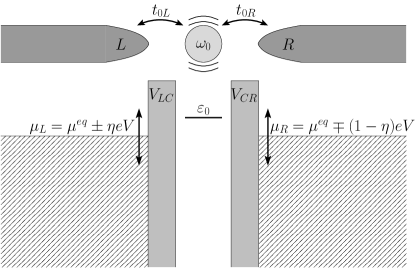
Figure 1: Schematic representation of the single site single mode (SSSM) model. The single electronic level $\varepsilon_{0}$ is broadened by the coupling to the leads; the electronic transport is resonant if the Fermi levels $\mu_{L,R}$ are very close to this broadened level, and off-resonant (as shown) otherwise. The system is shown in equilibrium, with $\mu_{L}=\mu_{R}$, non-equilibrium effects are studied by moving the Fermi levels.

The total Hamiltonian for the system is given by

$$H_{\text{total}}=H_{e}+H_{\text{vib}}+H_{{e\text{-vib}}},$$ (1)

where $H_{e},H_{\text{vib}}$ and $H_{{e\text{-vib}}}$ represent the electronic, vibron, and electron-vibron coupling parts of the Hamiltonian respectively. The electronic part of the Hamiltonian is broken into sections describing the left (right) electrode $H_{L}$ ($H_{R}$), the central interacting part $H_{C}^{e}$ and the potentials coupling the central region to the left and right electrodes $V_{LC}+V_{CR}$ respectively:

$$H_{e}=H_{L}+H_{C}^{e}+H_{R}+V_{LC}+V_{CR}.$$ (2)

The Hamiltonians for the electrodes are given by

$$H_{L}+H_{R}=\sum_{\alpha=L,R}\varepsilon_{\alpha}c^{\dagger}_{\alpha}c_{\alpha},$$ (3)

where $c^{\dagger}_{\alpha}$ ($c_{\alpha}$) creates (annihilates) a non-interacting electron with energy $\varepsilon$ on electrode $\alpha$. The electronic Hamiltonian for the central region and the coupling potentials are given by

$$H_{C}^{e}=H_{C}^{e}(\{d^{\dagger}_{n}\},\{d_{n}\}),$$ (4)

$$V_{LC}+V_{CR}=\sum_{n,\alpha=L,R}V_{\alpha n}c^{\dagger}_{\alpha}d_{n}+V^{*}_{\alpha n}d^{\dagger}_{n}c_{\alpha},$$ (5)

where the interacting electrons in the central region are created (annihilated) on electronic level $n$ by the operators $d^{\dagger}_{n}$ ($d_{n}$).

In principle, our Hamiltonian for the central region may contain electron-electron interactions, and is built from a complete set of single-electron creation and annihilation operators. In our current work we do not include any electron-electron interactions, and so the electronic part of the total Hamiltonian for the central region $H_{C}$ becomes

$$H_{C}^{e}=\sum_{n}\varepsilon_{n}d^{\dagger}_{n}d_{n}.$$ (6)

Meanwhile, the vibron part of the Hamiltonian is represented by

$$H_{\text{vib}}=\sum_{\lambda}\hbar\omega_{\lambda}a^{\dagger}_{\lambda}a_{\lambda},$$ (7)

where $a^{\dagger}_{\lambda}$ creates (annihilates) a vibron in vibron mode $\lambda$ with frequency $\omega_{\lambda}$. The electron-vibron coupling term is taken to be linear in the vibron displacement and its most general expression is then given by Ness et al. (2001)

$$H_{{e\text{-vib}}}=\sum_{\lambda,n,m}\gamma_{\lambda nm}(a^{\dagger}_{\lambda}+a_{\lambda})d^{\dagger}_{n}d_{m},$$ (8)

where $\gamma_{\lambda nm}$ is the coupling constant for exciting the vibron mode $\lambda$ by electronic transition between the electronic levels $n$ and $m$.

We concentrate on the simplest version of the Hamiltonian of the central part: the single-site single-mode SSSM model, in which one considers just one electron level coupled to one vibration mode. Despite the simplicity of this model, remarkably it not only contains all the physics we require but also ensures that we isolate the properties we are interested in without the complication of the added electronic levels. The reasons for this are as follows. Firstly, when the Fermi energy of the leads is pinned around the midgap, then at low and intermediate biases one of the frontier orbitals (either HOMO or LUMO) dominates the transport properties. Secondly in conjugated organic molecules (mostly used in single-molecule junction experiments), it is known that the optically relevant vibration modes are mostly coupled to either the HOMO or LUMO levels Heeger et al. (1988). We can therefore be confident that our model contains the relevant physics.

The total Hamiltonian for the central region thus becomes

$$H_{C}=\varepsilon_{0}d^{\dagger}d+\hbar\omega_{0}a^{\dagger}a+\gamma_{0}(a^{\dagger}+a)d^{\dagger}d,$$ (9)

where we now have just one electronic level $\varepsilon_{n}\rightarrow\varepsilon_{0}$ and just one vibron mode $a_{\lambda}\rightarrow a$, coupled via the electron-vibron coupling constant $\gamma_{0}$. The expression for the lead-central-region coupling (equation (5)) also simplifies to become

$$V_{LC}+V_{CR}=\sum_{\alpha=L,R}t_{0\alpha}(c^{\dagger}_{\alpha}d+d^{\dagger}c_{\alpha}),$$ (10)

where we have replaced the coupling potentials $V_{\alpha n}$ with hopping integrals $t_{0\alpha}$.

II.2 Non-equilibrium electron Green’s functions and electron-vibron self-energies

Non-equilibrium Green’s functions (NEGF) within the Keldysh formalism Keldysh (1965); Craig (1968); van Leeuwen et al. (2006); Rammer (2007) represent an extremely useful tool for studying the non-equilibrium properties of many-particle systems. The Green’s functions are functions of two space-time coordinates, and are obviously more complicated than the one-particle density which is the main ingredient of density-functional-based theories. One of the great advantage of NEGF techniques is that one can improve the calculations in a systematic way by taking into account specific physical processes (represented by Feynman diagrams) which is what we do in this paper for the electron-vibron interaction. The Green’s functions provide us directly with all expectation values of one-body operators (such as the density and the current), and also the total energy, the response functions, spectral functions, etc.

In Appendix A, we provide more details about NEGF and how to obtained the electron-vibron self-energies from a Feynman diagrammatic expansion of the electron-vibron interaction. We now briefly describe how we apply the NEGF formalism to the SSSM model.

The Green’s functions are calculated via Dyson-like equations. For the retarded and advanced Green’s functions $G^{r,a}$ these are

$$G^{r,a}=g^{r,a}_{C}+g^{r,a}_{C}\Sigma^{r,a}G^{r,a},$$ (11)

where $g^{r,a,}_{C}$ is the non-interacting Green’s function for the isolated central region.

For the greater $G^{>}$ and lesser $G^{<}$ Green’s functions, we use a quantum kinetic equation of the form

$$G^{>,<}=(1+G^{r}\Sigma^{r})g^{>,<}_{C}(1+\Sigma^{a}G^{a})+G^{r}\Sigma^{>,<}G^{a}.$$ (12)

Here $\Sigma^{x},(x=r,a,>,<)$ is a total self-energy consisting of a sum of the self-energies from the constituent parts of the system:

$$\Sigma^{x}=\Sigma^{x}_{L}+\Sigma^{x}_{R}+\Sigma^{x}_{\text{int}}.$$ (13)

$\Sigma^{x}_{L,R}$ are the self-energies arising from the non-interacting leads $\alpha=L,R$ and as such are simple to calculate:

$$\Sigma^{r}_{\alpha}=t_{0\alpha}^{2}g^{r}_{0\alpha}(\omega),$$ (14)

$$\Sigma^{a}_{\alpha}=(\Sigma^{r}_{\alpha})^{*},$$ (15)

$$\Sigma^{>}_{\alpha}=2i\ \Im m[\Sigma^{r}_{\alpha}(\omega)]\ (1-f_{\alpha}(\omega)),$$ (16)

$$\Sigma^{<}_{\alpha}=-2i\ \Im m[\Sigma^{r}_{\alpha}(\omega)]\ f_{\alpha}(\omega),$$ (17)

where $f_{\alpha}$ is the Fermi-Dirac distribution for lead $\alpha$, with Fermi level $\mu_{\alpha}=\mu^{\rm eq}+\eta_{\alpha}eV$ and temperature $T_{\alpha}$. The fraction of potential drop at the left contact is $\eta_{L}=\pm\eta_{V}$ and $\eta_{R}=\mp(1-\eta_{V})$ at the right contact Datta et al. (1997), hence $\eta_{L}-\eta_{R}=eV$ is indeed the applied bias, and $\eta_{V}\in[0,1]$.

The component of the retarded Green’s function for the isolated (non-interacting) lead $\alpha$ corresponding to the sites (or energy levels, depending on the representation used to the electrodes) connected to the central region is given by $g^{r}_{0\alpha}$.

In this paper, we have chosen a simple model, a semi-infinite tight-binding chain with on-site energy $\varepsilon_{\alpha}$ and nearest-neighbour hopping integral $\beta_{\alpha}$. This model gives a semi-elliptic density of states of the terminal lead site connected to the central region, and so each lead’s Green’s function becomes

$$g^{r}_{0\alpha}(\omega)=\exp({\rm i}k_{\alpha}(\omega))/\beta_{\alpha}\,$$ (18)

with $\omega=\varepsilon_{\alpha}+2\beta_{\alpha}\cos k_{\alpha}(\omega)$. We have chosen this model because it is one of the most simple, although in principle and in practice there are no limitations for taking any other more complicated or more realistic models for the lead, such as Bethe lattices with $z$-coordination, or a nanotip supported by a semi-infinite surface as shown in Ref Ness, 2006) since all their electronic properties are wrapped up in the lead self-energies $\Sigma^{x}_{L,R}(\omega)$.

The self-energy for the interacting central region, $\Sigma_{\text{int}}$ is somewhat more complicated. It consists of the sum of the self-energies due to interactions between the electrons and to interactions between the electrons and the quantum vibration modes (vibrons). In this paper we consider only the coupling between each electron and a single vibron of the central region (the molecule), hence the electron-vibron self-energy $\Sigma_{e\text{-vib}}$.

(a) $\Sigma_{e\text{-vib}}^{\text{Fock}}=$   (b) $\Sigma_{e\text{-vib}}^{\text{Hartree}}=$

Figure 2: The (a) Fock and (b) Hartree diagrams

(a) $\Sigma_{e\text{-vib}}^{\text{DX}}=$ (b) $\Sigma_{e\text{-vib}}^{\text{DPH}}=$

Figure 3: The (a) double exchange DX and (b) vibron propagator dressed by the e-h bubble diagrams (dressed phonon, DPH)

For the current work, it is necessary to calculate several types of self energy. Firstly we have the Fock-like self-energy $\Sigma_{{e\text{-vib}}}^{F,r/a/\gtrless}(\omega)$, which is a function of energy, and is represented in diagrammatic form by Figure 2(a). We also have the Hartree-like self-energy $\Sigma_{{e\text{-vib}}}^{H,r}$ which is independent of energy, given by Figure 2(b). Calculations using only the Hartree and Fock diagrams, and performed in a self-consistent way are usually referred to as the self-consistent Born approximation (SCBA) Mii et al. (2003); Frederiksen et al. (2004); Galperin et al. (2004a); Mitra et al. (2004); Pecchia et al. (2004); Chen et al. (2005b); Ryndyk and Keller (2005); Sergueev et al. (2005); Viljas et al. (2005); Yamamoto et al. (2005); Cresti et al. (2006); de la Vega et al. (2006); Egger and Gogolin (2008).

However, as explained in the introduction, we also want to go beyond the SCBA, and thus we will also calculate two further self-energies that include two-vibron processes. The first of these is the double-exchange self-energy $\Sigma^{\text{DX}}_{e\text{-vib}}$ given by Figure 3(a). In the many-body language, it is part of the vertex correction to the Fock diagram. The second is given by Figure 3(b) and corresponds to the dressed vibron (or GW-like) self-energy $\Sigma^{\text{DPH}}_{e\text{-vib}}$, which consists of the vibron propagator renormalized by a single electron-hole bubble (the polarization). This is why we refer to the effects of $\Sigma^{\text{DPH}}_{e\text{-vib}}$ as polarization effects in the following. The details of how we implement these self-energies are given in appendix A.

II.3 Physical properties

Once we have calculated all the different Green’s functions, any of the physical properties of the system, such as the electron density, the electronic current denstiy, the total energy, the current noise, the heat transfer, etc. can be calculated.

For example, the electronic current passing through the $\alpha$ contact is given by

$$I_{\alpha}(t)=\frac{2{\rm i}e}{\hbar}\sum_{n}V_{\alpha n}\langle c^{\dagger}_{\alpha}(t)d_{n}(t)\rangle-V^{*}_{\alpha n}\langle d^{\dagger}_{n}(t)c_{\alpha}(t)\rangle,$$ (19)

i.e the first term describes the transfer of an electron from the interacting region to electrode $\alpha$, while the second transfers an electron from electrode $\alpha$ to the central region.

We can then express this in terms of Green’s functions and derive an expression for the expectation value of the currentMeir and Wingreen (1992):

$$\begin{split}I_{\alpha}&=\frac{2e}{\hbar}\int\frac{{\rm d}\omega}{2\pi}\ {\rm Tr}\{\Sigma_{\alpha}^{<}(\omega)\ G^{>}(\omega)-\Sigma_{\alpha}^{>}(\omega)\ G^{<}(\omega)\}\\ &=\frac{{\rm i}2e}{\hbar}\int\frac{{\rm d}\omega}{2\pi}{\rm Tr}\left\{f_{\alpha}(\omega)\Gamma_{\alpha}(\omega)[G^{r}(\omega)-G^{a}(\omega)]\right.\\ &\qquad\quad\left.+\ \Gamma_{\alpha}(\omega)\ G^{<}(\omega)\right\}\ .\end{split}$$ (20)

All physical properties may be expressed in terms of the spectral function $A(\omega)$ which is at the heart of this paper. The spectral function is related to the imaginary part of the retarded or advanced electron Green’s functions, as

$$A(\omega)=-\Im m[G^{r}(\omega)]=+\Im m[G^{a}(\omega)]\ .$$ (21)

For non-interacting systems, it is simply proportional to the density of electronic states $n(\omega)=A(\omega)/\pi$. For interacting systems, it gives information about the excitations (electron or hole) of the system.

Furthermore, when the system is at equilibrium ($f_{L}=f_{R}=f^{\rm eq}$), there are some relationships between the lesser (greater) and the advanced and retarded Green’s functions:

$$\begin{split}G^{<,{\rm eq}}(\omega)=-f^{\rm eq}(\omega)\left(G^{r,{\rm eq}}(\omega)-G^{a,{\rm eq}}(\omega)\right)\\ =2{\rm i}f^{\rm eq}(\omega)A(\omega),\end{split}$$ (22)

and

$$\begin{split}G^{>,{\rm eq}}(\omega)=-(f^{\rm eq}(\omega)-1)\left(G^{r,{\rm eq}}(\omega)-G^{a,{\rm eq}}(\omega)\right)\\ =2{\rm i}(f^{\rm eq}(\omega)-1)A(\omega).\end{split}$$ (23)

These relationships are at the centre of the fluctuation-dissipation theorem for equilibrium, which also be recast as a relationship betweeen the greater and lesser Green’s functions:

$$G^{>,{\rm eq}}(\omega)\ =\ -{\rm e}^{(\omega-\mu_{0})/kT}\ G^{<,{\rm eq}}(\omega)$$ (24)

for statistical averages at finite temperature in the grand canonical ensemble. This equation is related to the Kubo-Martin-Schwinger boundary conditions Kadanoff and Baym (1962); van Leeuwen et al. (2006).

For non-equilibrium conditions, there is no unique Fermi level at finite bias (or no unique temperature if $T_{L}\neq T_{R}$) in the whole system, and the relationships given by Eqs. (22-24) no longer hold. This is an important feature of the non-equilibrium formalism for which conventional equilibrium statistics need to be reformulated.

II.4 Computational aspects

The calculations start by constructing the non-interacting Green’s functions of the entire system $G_{0}^{x}$ with $x$ being any three of the possible Green’s functions $x=\{r,a,<,>,t,\tilde{t}\}$. The other Green’s functions are obtained by using the relationships between them as shown in Appendix A.1. For example, the retarded Green’s function is given by $G^{r}_{0}(\omega)=[\ g^{r}_{0}(\omega)^{-1}-\Sigma^{r}_{\rm L}(\omega)-\Sigma^{r}_{\rm R}(\omega)]^{-1}$.

One then calculates three “Keldysh components” for the self-energies corresponding to any of the diagrams $\bigstar=$ {F,DX or DPH}: $\Sigma_{e\text{-vib}}^{\bigstar,<}$, $\Sigma_{e\text{-vib}}^{\bigstar,>}$ and $\Sigma_{e\text{-vib}}^{\bigstar,t}$. The Hartree diagram has only one component $\Sigma_{e\text{-vib}}^{H,r}$ as shown above.

The advanced and retarded self-energies $\Sigma_{e\text{-vib}}^{\bigstar,\{r,a\}}$ are then obtained by simple algebra using the relationships between the different self-energies as explained in Appendix A.1.

The new Green’s functions are then calculated by using the Dyson equations for $G^{r,a}$

$$G^{r,a}(\omega)=[\omega-\varepsilon_{0}-\Sigma_{\text{total}}^{r,a}(\omega)]^{-1},$$ (25)

and the quantum kinetic equations for $G^{<,>}$

$$G^{\gtrless}(\omega)=G^{r}(\omega)\Sigma_{\text{total}}^{\gtrless}(\omega)G^{a}(\omega),$$ (26)

where the total self-energies are given by

$$\Sigma_{\text{total}}^{x}(\omega)=\Sigma_{L}^{x}(\omega)+\Sigma_{R}^{x}(\omega)+\sum_{{\rm any}\bigstar}\Sigma_{e\text{-vib}}^{\bigstar,x}(\omega).$$ (27)

The new self-energies are then recalculated and the process re-iterates until full self-consistency is achieved.

Actually at each iteration of the calculations, we use a simple mixing scheme of the self-energies obtained at the present iteration and at the previous iteration. This mixing scheme permits us to achieve full self-consistency in a maybe slightly longer but more stable iterative process.

Note finally that by using Eq. 26, instead of the more general formulation given by Eq. 12, we assume that, after switching on the interactions, there are no bound states in the system (i.e. there are no interaction-induced electron states located outside the spectral supports of the left and right leads) Thygesen and Rubio (2007); Stefanucci (2007) which is indeed the case.

III Results: Spectral functions

In this section, we present results for the spectral functions $A(\omega)$ for the different transport regimes and for different applied biases in the low vibron-temperature regime.

We divide the calculations into four types. Firstly, we calculate the spectral functions at equilibrium for two transport regimes. The first of these is where $\varepsilon_{0}\gg\mu^{\rm eq}$ or $\varepsilon_{0}\ll\mu^{\rm eq}$, known as the off-resonant regime as in order to create a current between the left and right leads one puts an electron in the empty (for electron transport, $\varepsilon_{0}\gg\mu^{\rm eq}$) or full (for hole transport, $\varepsilon_{0}\ll\mu^{\rm eq}$) electronic level $\varepsilon_{0}$.

The second transport regime is when $\varepsilon_{0}\pm\text{linewidth}\sim\mu^{\rm eq}$, known as the resonant transport regime. The linewidth is the width of the peak in the spectral function which arises from the electronic coupling of the central region to the left and right leads. In this case the electronic level $\varepsilon_{0}$ is, at equilibrium, half-filled by an electron (and thus also half-filled with a hole).

For each of these transport regimes, we calculate the spectral function both at equilibrium (applied bias $V=0$) and non-equilibrium at finite bias ($V>0$).

For each of these four groups (resonant/off-resonant transport regimes, at/out of equilibrium), a large amount of different NEGF calculations have been performed for different values of the relevant parameters and within different levels of approximation (Hartree Fock, Hartree Fock+second-order, partially or fully self-consistent calculations). In the rest of this section, we present only a limited and selected number of results which we found the most relevant for each case, and we analyse and compare in detail the effects of the different diagrams on the spectral functions of the system at and out of equilibrium.

We also, in section III.3, compare perturbation expansion based calculations (NEGF) to a reference calculation which is exact in term of electron-vibron coupling but which however is only valid for a specific transport regime.

III.1 At equilibrium

We first consider the spectral functions at equilibrium, with no applied bias. Figure 4 shows $A(\omega)$ for the off-resonant regime, and Figure 5 shows the resonant transport regime.

In the equilibrium many-body language, the features in the spectral functions obtained at positive energies ($\omega\geq 0$, above the Fermi level) correspond to electron excitations, while the features at negative energies ($\omega\leq 0$, below the Fermi level) correspond to hole excitations.

III.1.1 Off-resonant transport regime

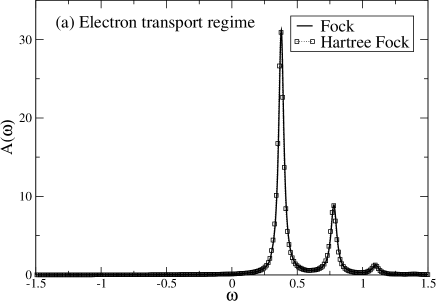
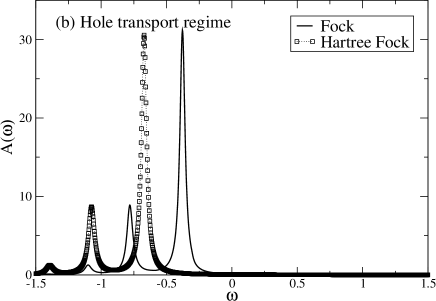
Figure 4: Equilibrium (zero bias) spectral functions $A(\omega)$ for the off-resonant (a) electron and (b) hole transport regime. Calculations were performed with the Fock-like electron-vibron diagram (solid line) and with both the Hartree and Fock-like diagrams (symbols and dotted line). For the electron transport regime the inclusion of the Hartree self-energy has no effect, but for the hole transport regime it shifts the entire spectral function to lower energies. The parameters are $\varepsilon_{0}=+0.5(-0.5)$ for electron (hole) transport $\gamma_{0}=0.21,\omega_{0}=0.3,t_{0L,R}=0.15,\eta=0.005$ and $\mu_{L}=\mu_{R}=\mu^{\rm eq}=0$.

For the off-resonant electron transport regime (Figure 4(a)) all the features in the spectral function are above the Fermi level $\mu^{\rm eq}$ and hence correspond to electron excitations. The main peak corresponds to adding an electron in the single available level. This peak is broadened by the coupling to the leads, and its position in energy $\tilde{\varepsilon}_{0}$ is renormalised by the electron-vibron interaction, i.e. $\tilde{\varepsilon}_{0}$ is close to the static the polaron shift $\tilde{\varepsilon}_{0}\approx\varepsilon_{0}-\gamma_{0}^{2}/\omega_{0}$.

The lesser peaks in the electron-transport spectral function are vibron side-band peaks arising from resonance with $n=1,2,3,...$ excitations in the vibration mode. These peaks correspond to vibration excitation (vibron emission) only. At zero vibron temperature, these are the only available mechanisms for vibrational excitations. We note, and discuss further in section III.3, that these side-band peaks should occur at integer multiples of $\omega_{0}$ away from the main peak, but that for both our Fock-only and Hartree-Fock SCBA calculations the peak-peak separation is slightly wider than this.

In this regime, the Hartree self-energy is negligible, because most of the spectral weight is above the Fermi level and $\Sigma^{H}_{e\text{-vib}}\propto\int^{\mu^{\rm eq}}{\rm d}\omega A(\omega)\sim 0$. This implies that the polaron shift is mainly due to the Fock-like self-energy.

For the off-resonant hole-transport regime ( Figure 4(b)), all the features in the spectral function occur at $\omega<0$ and therefore correspond to hole excitations. The vibron side band peaks are at lower frequencies than the main peak because they correspond to the emission of vibrons by holes rather than electrons.

When we include just the Fock-like self-energy, the hole spectral function is symmetric (with respect to the equilibrium Fermi level $\mu^{\rm eq}$) with the electron spectral function, as can be seen clearly in figure 5. Adding the Hartree self-energy, however, breaks this electron-hole symmetry. As most of the spectral weight is below $\mu^{\text{eq}}$, the expression for $\Sigma^{H}_{e\text{-vib}}$ given in equation Eq.(46) reduces to a constant $2\gamma_{0}^{2}/\omega_{0}$ (i.e. twice the polaron shift) as $\int\frac{d\omega}{2\pi}\rm{i}G^{<}(\omega)\sim 1$. As a result of this the whole spectral function is shifted to the left by this amount.

III.1.2 Resonant transport regime

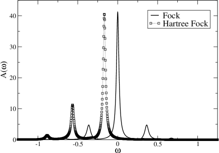
Figure 5: Equilibrium spectral function $A(\omega)$ for the resonant transport regime. Calculations were performed with the Fock-like (solid line) and with both the Hartree and Fock-like diagrams (dashed line). The parameters are identical to those used in Figure 4, except for the value of the electron level which is $\varepsilon_{0}=0$ for the resonant regime.

We now turn to the resonant transport regime, with the spectral function shown in Figure 5. Here our electronic level $\varepsilon_{0}$ is broadened by the coupling to the leads and is partially filled with electrons. We can see that calculations performed with only the Fock-like self-energy preserve the electron-hole symmetry. The spectral function presents peaks located both at positive and negative energies, which correspond to the emission of vibrons by electrons or holes respectively. As in the previous section, the inclusion of the Hartree self-energy (equation  (46)) breaks down the electron-hole symmetry and the features are shifted to lower energies with a corresponding modification of the spectral weights for each peak.

We note here that the inclusion of the Hartree self-energy thus modifies so drastically the spectral function that it will also strongly affect the $I$-$V$ characteristics of the junction in comparison to calculations performed with only the Fock self-energy .

III.2 Non-equilibrium spectral functions

III.2.1 Non-equilibrium off-resonant transport

In this section, we present results for the spectral functions $A(\omega)$ for the off-resonant transport regimes, for different applied biases, both with and without the Hartree contribution. We first present calculations for an asymmetric potential drop with $\eta_{V}=1$, i.e. $\mu_{L}=V$ and $\mu_{R}=0$ ($\mu^{\rm eq}=0$).

Figure 6(a) shows the spectral function calculated with just the Fock component at different applied biases. We then increase the bias $V$ by increasing the chemical potential of the left contact while keeping that of the right contact at zero. For low values of $V$ ($V\leq\omega_{0}$) there is little change in the spectral function. However, once the value of $V$ exceeds that of $\omega_{0}$, the spectral function becomes increasingly modified, especially when there is significant spectral weight inside the bias window $\mu_{R}<\omega<\mu_{L}$. In particular, the lineshapes of both the main peak and the vibron side-band peaks become deformed, with a noticeable asymmetry of the main peak for biases where the main peak, but not the right-hand vibron side-band peak, lies within the bias window.

There is a saturation regime once the vibron side band peaks, and thus nearly all of the spectral weight, is within the bias window (curves for $\mu_{R}\gtrsim 1$). Here the main peak becomes pinned around $\omega=0.5$ (effectively midway between $\mu_{L}$ and $\mu_{R}$), and a symmetric lineshape is restored. We postulate that this is owing to the bias being large enough to achieve simultaneous electron and hole transport.

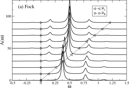
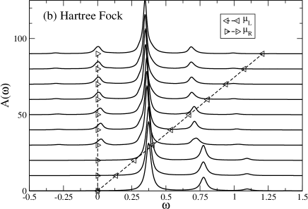
Figure 6: Non-equilibrium spectral function for the off-resonant transport regime with applied bias for (a) the Fock diagram only and (b) both Fock and Hartree diagrams. The curves are offset vertically for clarity. The applied bias is given by the chemical potentials of the left (left-pointing arrows) and right (right-pointing arrows) leads respectively. The Hartree potential has a strong effect on the peak positions. The other parameters are $\varepsilon_{0}=+0.5,\gamma_{0}=0.21,\omega_{0}=0.3,t_{0L,R}=0.15,\eta=0.005,\eta_{V}=1$.

Figure 6(b) shows the spectral function with both the Hartree and Fock diagrams included. As we have already noted, at zero bias there is no change from the Fock-only spectral function. For small biases ($V\lesssim\omega_{0}$) there is little difference, but for larger biases the effect of the Fock diagram becomes increasingly evident. This is because once the bias exceeds the vibron frequency $\omega_{0}$, the non-equilibrium electron density becomes strongly perturbed. The main peak is more stable in position than for the Fock-only spectral function, although it shifts slightly towards lower energies with increasing bias before stabilising. The righthand vibron side-band peak becomes strongly deformed, and moves to lower, rather than higher, energies as the bias is increased. The left-hand vibron side-band peak appears at a lower bias than for the Fock-only spectral function, at a frequency just above zero, then tends towards zero as the bias increases. As for the Fock-only case however, once both vibron side-band peaks are within the bias window, saturation is reached and the peak positions stabilize. For both the Fock-only and Hartree-Fock spectral functions, the separation between both side-band peaks and the main peak is $\sim 0.34,>\omega_{0}$ for the parameters we used.

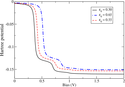
Figure 7: (color online) Hartree potential versus applied bias. The Hartree potential is almost constant in the low bias regime, and hence it could be neglected in the calculations, because it just corresponds to a global energy reference shift. However for larger biases, it is much more influential as the non-equilibrium electron density varies a lot with the applied bias. The parameters are the same as in figure 6.

Figure 7 shows the Hartree potential (i.e. the real part of $\Sigma_{e\text{-vib}}^{H,r}$) plotted against applied bias for different values of the electronic level $\varepsilon_{0}$. The solid line corresponds to the value of $\varepsilon_{0}$ used to calculate the spectral functions of the lower panel in Figure 6. The Hartree potential is small and almost constant in the low bias region. Hence, in the quasi-equilibrium regime, such a potential could be neglected in the calculations, because it simply corresponds to an energy reference shift. However when the bias window $[\mu_{L},\mu_{R}]$ starts to encompass features in the spectral functions (either the main peak or vibron side-band peaks), the corresponding non-equilibrium electron density starts to vary substantially with the applied bias. Thus the Hartree potential shows a strong dependence on the value of the bias (as also shown in Ref. [Lee et al., 2009]), until the saturation regime is reached and the Hartree potential is once again constant for very large biases. The asymptotic saturation value of the Hartree potential is dependent on the value of the electronic level $\varepsilon_{0}$ as one would expect. The first drop in the value of the Hartree potential happens at $\tilde{\varepsilon}_{0}$, with the subsequent steps, which become progressively smaller and broader, at $\tilde{\varepsilon}_{0}+\sim 0.34$ and then $\tilde{\varepsilon}_{0}+n\omega_{0}$.

This behaviour indicates that one cannot in principle neglect the Hartree diagram contribution in the calculations, unless one is interested in calculating only the properties of the system for a bias range for which the electron density is (almost) constant .

It is worth mentioning that it is not straightforward to relate the modification of the peak positions in the two panels in figure 6 to the Hartree potential alone. In self-consistent calculations, a highly non-linear system needs to be solved, since the Hartree potential is obtained from one element of the Green’s functions which are themselves dependent on the values of the Hartree potential.

III.2.2 Non-equilibrium resonant transport

We now consider what happens when we apply a bias in the resonant transport regime. We apply a symmetric potential drop (i.e. the potential of the left electrode is raised by an amount $\eta eV$ while that of the right electrode drops by the same amount). This allows us to keep the electron-hole symmetry and see under which circumstances the electron-hole symmetry is broken.

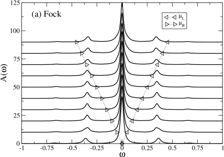
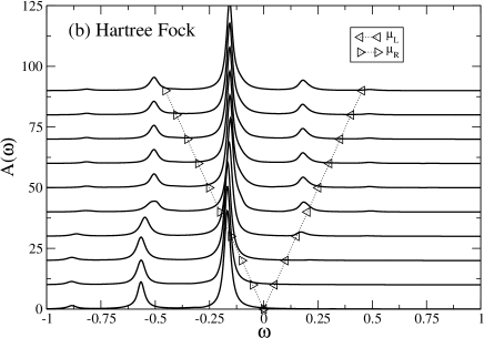
Figure 8: Non-equilibrium spectral function $A(\omega)$ for the resonant transport regime for different applied biases for (a) the Fock diagram only, and (b) the Fock and Hartree diagrams. The curves are shifted vertically (+10 in $y$-axis) for clarity, with the values of the left and right chemical potentials given by the triangular symbols, here we have a symmetric potential drop. Adding the Hartree diagram breaks the electron-hole symmetry. The other parameters are the same as for Figure 6 except for $\varepsilon_{0}=+0$ and $\eta_{V}=0.5$.

The spectral functions for the Fock diagram are shown in figure 8(a). As we have no Hartree term, the spectral function is electron-hole symmetric at equilibrium. Moreover, as we have chosen a symmetric potential drop ($\eta=0.5$) the spectral functions stay symmetric for all applied biases. Constraining the symmetry in this way allows us to concentrate on the effects of increasing the bias, and we can see that the most important modifications of the spectral function are in the width of the central and satellite peaks. The vibron side-band peaks show only a very small change with increasing applied bias.

Figure 8(b) shows the spectral function when we add in the Hartree term while keeping all other variables unchanged. We note immediately that the electron-hole symmetry is broken, even at equilibrium. In addition the main peak is shifted towards negative energies with respect to the Fock-only calculation, and the right-hand vibron side-band peak is completely suppressed—the whole spectral function takes on the qualitative appearance of a spectral function in the hole-dominated regime (compare with Figure 4). On increasing the bias, the width and shape of the left-hand vibron side-band peaks is varied, and for higher biases new vibron side-band peaks appear above the main peak, until at high biases the spectral function is very similar in shape to that for the off-resonant spectral function (Figure 6).

III.3 A comparison with inelastic scattering techniques

In this section, we will check the validity of the self-consistent Born approximation (SCBA), i.e. self-consistent calculations using only the Hartree and Fock diagrams, versus another method which gives more exact results as far as electron-vibron coupling is concerned. Since NEGF is a many-body perturbation expansion theory, by definition it does not contain all diagrams even though self-consistency allows us to achieve a partial resummation of a subclass of diagrams.

As an alternative to NEGF, one can calculate the transport properties using an extension of conventional scattering theory to include the interaction of incoming single-particle states with some bosonic degrees of freedom inside the central region of interest Bonča and Trugman (1995); Ness et al. (2001); Ness (2006).

This technique, termed the multi-channel inelastic scattering technique (MCIST) Ness et al. (2001); Ness (2006), has the advantage of being an exactly solvable problem, even in the presence of many non-interacting electronic states coupled to many vibration modes in the central region Ness et al. (2001). MCIST is based on many-body perturbation theory for polaron and it is exactly solvable in the sense that MCIST is treating the electron-vibron coupling to all orders. In the language of polaron theory, MCIST contains all the diagrams corresponding to the electron-vibron interaction (in the corresponding transport regime). To be more precise, MCIST contains all orders of crossing and non-crossing diagrams in terms of the bare vibron propagator Ness (2006); Ciuchi et al. (1997); Cini and D’Andrea (1988); Smondyrev (1986). In conventional polaron theory for one electron, there are no diagrams with electron-hole loops in them Smondyrev (1986).

However, MCIST is a single-particle scattering technique and treats the statistics of the Fermi seas of the left and right leads only in an approximate manner. In the language of NEGF, this means that the results given by MCIST are only valid for a specific transport regime (as we will see below).

In the case of the SSSM model, the retarded Green’s function of the central region has the usual form

$$G^{r}(\omega)=[\ g^{r}_{0}(\omega)^{-1}-\Sigma^{r}_{\rm leads}(\omega)-\Sigma^{r}_{{e\text{-vib}}}(\omega)]^{-1}\ .$$ (28)

Within MCIST, the retarded electron-vibron self-energy containing all orders of the electron-vibron coupling is expressed as a continued-fraction as shown analytically in Refs. [Ness, 2006] and [Cini and D’Andrea, 1988]:

$$\begin{split}&\Sigma^{r}_{{e\text{-vib}}}(\omega)=\\ &\cfrac{\gamma_{0}^{2}}{G^{r}_{0}(\omega-\omega_{0})^{-1}-\cfrac{2\gamma_{0}^{2}}{G^{r}_{0}(\omega-2\omega_{0})^{-1}-\cfrac{3\gamma_{0}^{2}}{G^{r}_{0}(\omega-3\omega_{0})^{-1}-...}}}\end{split}$$ (29)

where we recall that $G^{r}_{0}$ is the retarded GF of the central region connected to the leads, i.e. $G^{r}_{0}(\omega)=[\ g^{r}_{0}(\omega)^{-1}-\Sigma^{r}_{\rm leads}(\omega)]^{-1}$, without electron-vibron coupling.

As show in Ref. [Ness, 2006], the lowest Born approximation, fully consistent with SCBA (Hartree-Fock calculations as shown above), is given in MCIST by an electron-vibron self-energy equivalent to Eq. (29) but where the integer $n$ factors at each level of the continued fraction are all replaced by the integer $n=1$.

Obviously, this approximate substitution is good enough in the (very) weak electron-vibron coupling for which only the first level of the continued fraction contributes the most Ness (2006).

Below we compare the spectral functions obtained by exact MCIST calculations, by MCIST approximated to the SCBA (Hartree-Fock) level, and to NEGF-SCBA calculations.

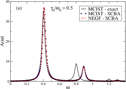
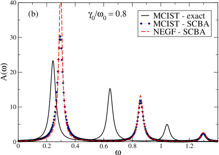
Figure 9: (Color online) Equilibrium off-resonant spectral functions calculated with the MCIST technique and NEGF-SCBA for the off-resonant regime. The upper panel shows results for weak electron-vibron coupling ($\gamma_{0}/\omega_{0}=0.5$), while the lower panel shows results for strong electron-vibron coupling ($\gamma_{0}/\omega_{0}=0.8$). MCIST calculations give exact results in this case, and can also be performed at the same level of approximation as SCBA (see main text for details). MCIST-SCBA and NEGF-SCBA are virtually identical, but show large discrepancies for the peak positions (main peak and more especially for the vibron side-band peaks) in comparison to the exact results. The parameters are $\varepsilon_{0}=+0.5$ (electron transport), $\gamma_{0}=0.2$ (upper panel) and $\gamma_{0}=0.32$ (lower panel), $\omega_{0}=0.4,t_{0L,R}=0.15$.

The spectral functions obtained from MCIST are shown in figure 9 for the weak/intermediate electron-vibron coupling regime ($\gamma_{0}/\omega_{0}=0.5$) and for the strong electron-vibron coupling regime ($\gamma_{0}/\omega_{0}=0.8$). The overall lineshapes correspond to a main peak with vibron side-band peaks located only above the main peak. These are typical results fully consistent with an off-resonant transport regime situation. Furthermore, the spectral functions obtained with BA-based approximation (MCIST-SCBA and NEGF-SCBA) are virtually identical, especially in the intermediate ($\gamma_{0}/\omega_{0}=0.5$) to very weak (not shown here) electron-vibron coupling regime. For strong electron-vibron coupling, one obtains the same peak positions, however the amplitude of the peaks (especially the main peak) is slightly different.

Since MCIST calculations will always give similar lineshapes independent of the value of $\varepsilon_{0}$, one can conclude that MCIST calculations are only valid for the off-resonant transport regime at and near equilibrium. MCIST is not able to reproduce the spectral features of the resonant transport regime (i.e. vibron side-band peaks on both sides of the main peak). This is essentially due to the fact that in MCIST, one does not take properly into account the statistics of the Fermi seas of the left and right leads. See for example Eqs. (28) and (29), there are no leads’ Fermi distributions in the retarded component of the leads’ self-energies $\Sigma^{r}_{L,R}$.

Now, comparing BA-based calculations with the exact MCIST calculations, one can see from figure 9 that the BA-based calculations give the wrong polaron shift, i.e. the normalized position of the main peak $\varepsilon_{0}$, especially in the strong electron-vibron coupling regime. Furthermore BA-based calculations also give the wrong energy separation between the main peak and the first vibron side-band peak. This energy difference should be equal to the vibron energy $\omega_{0}$, as it is given by exact MCIST calculations. Note that the limits of BA-based calculations were also been studied by Lee et al. in a somewhat different context in Ref. [Lee et al., 2009].

In conclusion, this means that Hartree-Fock (or BA) based calculations for electron-vibron interaction are only valid for weak coupling, as can be expected from a perturbation-expansion based theory. Hence one needs to include higher-order diagrams in the electron-vibron self-energies to go beyond the commonly-used self-consistent Born approximation (Hartree-Fock) in order to obtain correct results for a wide range of parameters. The effects of the higher-order diagrams (here second-order-DX and DPH diagrams) are explored in detail in the following sections.

Additionally, although MCIST calculations are only valid in the off-resonant transport regime at and near equilibrium, they include all possible higher-order diagrams (with bare vibron propagator) and hence can be used as a reference for any perturbation-expansion-based NEGF calculations performed at equilibrium or in the quasi-equilibrium regime.

III.4 Vertex corrections and polarization effects to the spectral functions

In this section, we present results for the spectral functions when the second-order diagrams (see Figure 3) are included in the calculations of the Green’s functions. The reader can find more information about the mathematical expressions for the self-energies corresponding to the second-order diagrams in Appendix A.

These diagrams fall into two types—the double-exchange DX diagram, corresponding to vertex corrections, and the dressed vibron diagram, which includes a single electron-hole bubble, renormalizing the vibron propagator and hence giving rise to polarization effects.

We have used three different levels of approximation to calculate these Green’s functions: Firstly, calculations with no self-consistency—the Green’s functions are simply calculated using the diagrams in Figure 2 and Figure 3 using the bare propagator $G_{0}$ as the electron Green’s function. In our model, $G_{0}$ is the Green’s function of the central region connected to the leads with no electron-vibron interactions. This is a first-order perturbation expansion for which $\Sigma_{e\text{-vib}}^{H,F,DX,\ {\rm and/or}\ DP}[G_{0}]$. We use the abbreviations BA (Born approximation for non self-consistent Hartree and Fock diagrams) and BA+DX (DX for double exchange) and BA+DX+DPH (DPH for dressed vibron, for the $GW$-like diagram) in the following.

Secondly, we perform partly self-consistent calculations, where the Green’s functions are calculated with the first loop of self-consistent calculations with the Hartree and Fock diagrams. We use these Green’s functions as a starting point to calculate new, corrected, Green’s functions including the second-order diagrams $\Sigma_{e\text{-vib}}^{\text{DX}}$ and/or $\Sigma^{GW}_{e\text{-vib}}[G^{SCBA}]$ in which the Green’s functions are the corresponding SCBA Green’s functions.

Finally, we perform fully self-consistent calculations, in which the Green’s functions are calculated in a self-consistent manner with the first and second-order diagrams included within each iteration of the self-consistency loop.

Our rationale for choosing to do calculations in this manner is as follows. We are able to test the different levels of approximation and see very precisely the effects of vertex corrections and polarization are on both the bare Green’s functions $G_{0}$ and the SCBA-level Green’s functions. We will also show in section III.4.1 that by using the SCBA Green’s functions rather than $G_{0}$ as a starting point, one achieve a better convergence in the calculations. In particular we will show later on in Section III.4.1 that in some cases, for example the off-resonant transport regime when $\gamma_{0}/\omega_{0}\gtrsim 0.6-0.7$), the use of the bare $G_{0}$ Green’s functions as a starting point for a fully self-consistent calculation with second-order diagrams actually gives unphysical results. Additionally, fully self-consistent calculations are extremely computationally intensive, and hence it is both interesting and useful to explore the range of parameters for which the second-order-diagram corrections to the SCBA calculations give a sufficiently accurate description of the Green’s functions in comparison to the fully self-consistent calculations.

III.4.1 Off-resonant regime at equilibrium

Figure 10 shows the spectral functions of the off-resonant transport regime at equilibrium, calculated for weak/intermediate electron-vibron coupling ($\gamma_{0}/\omega_{0}=0.50$) and for different diagrams and levels of self-consistency.

As already mentioned in sections III.1 and III.2, the energy separation between the main peak and the first vibron side-band peak (which should be equal to the vibron energy, here $\omega_{0}=0.40$) is not well reproduced by BA-based (Hartree-Fock based) calculations and is much larger than $\omega_{0}$. The self-consistency introduced in the calculations give a marginally smaller energy separation.

The effects of the second-order DX diagram are firstly to bring the vibron side-band peak closer to the main peak, hence giving an energy separation closer to the exact value; and secondly, one observes a strong narrowing and a larger amplitude of the vibron side-band peak in both self-consistent and non-self-consistent calculations. Both these effects thus qualitatively modify the spectral functions towards better agreement with the exact results as shown in Section III.3.

It is, however, worth mentioning that including the DX diagram in the calculation does not greatly affect the position of the main peak, a result which may be understood from the fact that the dynamical polaron shift is a quantity difficult to obtain exactly from a perturbation expansion theory beyond weak coupling Ness (2006); Smondyrev (1986).

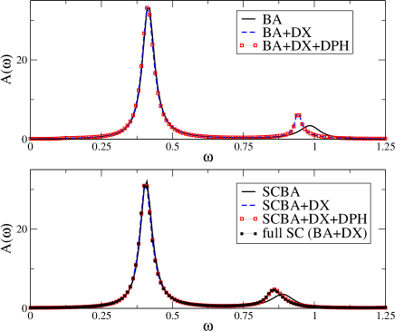
Figure 10: (Color online) Equilibrium spectral function for the off-resonant electron transport regime in the weak/intermediate electron-vibron coupling. Non self-consistent (top panel) and self-consistent (bottom panel) calculations were performed with first-order Hartree and Fock-like (BA, solid lines), plus second-order DX (dashed lines), plus DPH (squares) electron-vibron self-energy diagrams. The other parameters are $\varepsilon_{0}=+0.5$, $\gamma_{0}=0.2,\omega_{0}=0.4,t_{0L,R}=0.15,\eta=0.025$. Self-consistent calculations give better spectral functions, with vibron side-band peak closer to the main peak. The second-order DX diagram narrows the side-band peaks and bring them even closer to the main peak as expected. The second-order DPH diagram does not contribute much in the off-resonant regime. In this regime and for small electron-vibron coupling, second-order corrections to SCBA calculations are a good approximation to corresponding full self-consistent calculations.

The effects of the second-order DPH diagram in the spectral function are virtually nil for the case of weak/intermediate coupling and the off-resonant regime. This might not be that surprising since the DPH diagram corresponds to a Fock-like diagram with a renormalised vibron propagator. The renormalization of the vibron is due to a single electron-hole bubble. However in the off-resonant transport regime, the spectral function is almost empty (in the case of electron transport) or almost full (in the case of hole transport) which implies that there are not many electron-hole excitations available in this transport regime. Hence the polarization (i.e. the contribution of the electron-hole bubble) is very small, subsequently giving very small values for the DPH self-energy. As an example, we have checked our numerical values in the case shown in figure 10 and we have found, as expected, that the maximum values of $\Sigma_{e\text{-vib}}^{{\rm DPH},r}$ are 30 to 50 times smaller than the maximum values of $\Sigma_{e\text{-vib}}^{{\rm DX},r}$.

Furthermore, in the off-resonant regime and for weak-ish electron-vibron coupling, it seems that the fully self-consistent (full SC (BA+DX) curve in figure 10) results $G_{\rm full\ SC}^{r}(\omega)$ are well approximated by the results given by a second-order correction to a self-consistent Hartree-Fock (SCBA) calculations (SCBA+DX curve in figure 10) $G_{\rm partial\ SC}^{r}(\omega)=[G_{\rm SCBA}^{r}(\omega)^{-1}-\Sigma^{{\rm DX},r}[G_{\rm SCBA}]\ ]^{-1}$. This is an interesting result as it implies that the physical properties of the system, at least in these conditions, could be well described by a second-order correction of the lowest-order SC calculations, without the need to perform a fully self-consistent calculation up to the second-order.

Now we turn to the analysis of results obtained for stronger electron-vibron coupling. Examples of such calculations are given in figure 11 for $\gamma_{0}/\omega_{0}=0.80$. In the strong electron-vibron coupling regime, one obtains qualitatively the same contributions of the second-order diagrams as explained above for the weak coupling regime. The DPH diagram does not have a large role in the off-resonant transport regime, although slightly affecting the width of the main peak. And the DX diagram shifts the vibron side-band peak towards the main peak (and hence towards the exact results) as well as narrowing the peak width and increasing the peak amplitude. These effects are amplified in Figure 11 because the electron-vibron coupling constant $\gamma_{0}$ is bigger than in Figure 10. Furthermore, for strong electron-vibron coupling, the DX diagram modifies the energy position of the main peak and seems to give a slightly better polaron shift.

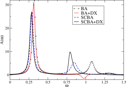
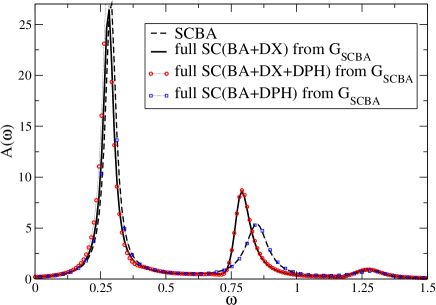
Figure 11: Equilibrium spectral function for the off-resonant electron transport regime and strong electron-vibron coupling. Calculations were performed with different diagrams: first-order Hartree and Fock-like (BA) and second-order (DX, DPH) electron-vibron self-energy diagrams. (Top panel): Calculations were done with no self-consistency (BA,BA+DX), partial (SCBA+DX) and full self-consistency (SCBA). (Bottom panel): full self-consistent SC(BA+…) calculations. The other parameters are $\varepsilon_{0}=+0.5$, $\gamma_{0}=0.32,\omega_{0}=0.4,t_{0L,R}=0.15,\eta=0.025$. The calculations show that no self-consistency gives poor results in comparison to exact calculations given in Figure 9. A closer spectral function to the exact result is obtained from SC(BA+DX) calculation. The second-order DPH diagram do not contribute much in the off-resonant regime. See main text for a detailed analysis of the spectral functions.

There is however another interesting effect observed from such a set of calculations, which can be seen in the upper panel of Figure 11. The first iteration of a fully self-consistent calculation (including the Hartree, Fock, and DX diagrams) starting with the non-interacting GFs $G_{0}$ gives non physical results, i.e. negative values of the spectral function (see curve BA+DX in figure 11), and such an unphysical behaviour does not self-correct in the following iterations. This a well known problem, which has already been encountered in the past by several authors in the context of electron-vibron interaction (for example in Ref [Král, 1997]) and also in the context of electron-electron interaction when considering topologically equivalent diagrams Shirley and Martin (1993); Shirley (1996) . In Ref. [Král, 1997], a somewhat different approach than ours was used. It is based on a linked cluster expansion for the non-equilibrium steady-state regime, and negative densities of states were obtained when including second-order diagrams, and in some cases even higher-order cluster approximations did not seem to give a convergent solution at intermediate electron-vibron strength and in the presence of the Fermi seas.

However, our calculations reveal that it is possible to solve such a problem by starting the fully self-consistent calculations (up to second order) from a different starting point, namely by starting from the $G_{\rm SCBA}$ Green’s functions (i.e. the GFs obtained from a fully SC calculation including only the lowest-order diagrams). This is shown by the curve (SCBA+DX) in the upper panel of figure 11 and by the lower panel in which all the fully converged self-consistent results are shown.

For the moment, we do not have a full physical explanation of the reason why starting from a SCBA calculations is better to achieve full self-consistency with higher-order diagram than Hartree-Fock, apart from the simple fact that an Hartree-Fock calculation is probably closer to the true interacting solution than the non-interacting solution.

To conclude this section, we can say that in the off-resonant regime at equilibrium, the second-order DX diagram dominates over the second order DPH diagram.

III.4.2 Resonant regime at equilibrium

In this section, we present calculations for the resonant regime at equilibrium. Though we have shown, in sections III.1.2 and III.2.2, the importance of the Hartree diagram, we will consider below results obtained without the Hartree diagram. The calculations were performed with the Fock and second-order DX and/or DPH diagrams which conserve (at numerical accuracy) the electron-hole symmetry of the system.

The reasons why we have choosen to perform this model calculation are twofold: first, even for a single electronic level, we expect to have the maximum possible electron-hole excitations available when the spectral functions are electron-hole symmetric. Hence we expect the polarization effects be to more pronounced in a system with electron-hole symmetry. Second, the electron-hole symmetric model permits us to emphasize the competitive effects between the DX and DPH diagrams as will be shown below.

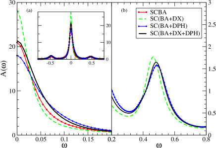
Figure 12: (color online). Equilibrium spectral function for the resonant transport regime and weak/intermediate electron-vibron coupling. Calculations were performed with diagrams: BA (Hartree-Fock) and second-order DX, DPH electron-vibron diagrams. The other parameters are $\varepsilon_{0}=+0.0$ (resonant transport), $\gamma_{0}=0.24,\omega_{0}=0.4,t_{0L,R}=0.2,\eta=0.03$. The top inset shows the whole spectral functions, while the left (a) and right (b) parts are zooms, for positive $\omega$, of the central peak and first vibron side-band peak respectively. The second-order diagrams have the following effects on the SCBA spectral functions: DPH broadens the central and side-band peaks as well as lowers their height, in opposition to DX which narrows the peaks and brings the side-band peaks slightly closer to the center, with a strong and unphysical increase of the amplitude of the central peak. Calculations with both DX and DPH give in appearance a broadening of the central peak, which however recovers the correct height necessary to conserve the Fermi-liquid property of the electron-hole symmetric system (see Section III.5 for more detail).

Figure 12 shows the equilibrium spectral functions of the resonant regime (at weak/intermediate electron-vibron coupling) obtained from different self-consistent calculations including first and second-order diagrams.

On one hand, the second-order DPH diagram corresponds to a partial dressing of the vibron propagator by one electron-hole bubble. It gives an extra lifetime in the retarded/advanced electron Green’s functions in comparison to Hartree-Fock (SCBA) calculations. Hence the main effect of the DPH diagram is to introduce an extra broadening of the peaks in the spectral functions. Since the DPH diagram is one of the so-called conserving approximations Baym (1962); Kadanoff and Baym (1962), the broadening of the peaks leads to a reduction of their height to keep globally the same total spectral weight. These effects can be seen on the SC(BA+DPH) curve in Figure 12.

On the other hand, the second-order DX diagram, which is a conserving approximation, has an opposite effect: a strong narrowing of the peaks (especially of the central peak) accompanied with an increase of their height, as can seen on the SC(BA+DX) curve in Figure 12.

Now it is interesting to see what happens when the calculations are performed with both second-order DX and DPH diagrams. This is shown on the SC(BA+DX+DPH) curve in Figure 12: We obtain a hybrid behaviour, in the sense that in appearance the central peak is broadened in comparison to SCBA calculations. However, the height of the peak at the Fermi level is conserved (up to numerical accuracy). This is a very important result which proves that for the model calculation of an electron-hole symmetric system, one has to include both the DX and DPH second-order diagrams in order to conserve the expected Fermi-liquid properties of the system. In this regime both the DX and DPH second-order diagrams play an equally important role which determines the linear response properties of the system as shown below in Section III.5.

By comparison, in a diagrammatic treatment of the electron-electron interaction on the electron propagator, the situation is often different: the electron-hole bubble diagram that appears here in the DPH contribution to the propagator is large, especially in highly polarizable metallic and open-shell systems where electron-hole pairs may be created with low energy cost, because the Coulomb interaction operates at all energy scales. In that case, summing the bubble diagrams to infinite order as is done in Hedin’s $GW$ approximation Hedin (1965); Hedin and Lundqvist (1969) is much more important than including the second-order exchange diagram. The key difference for the electron-phonon interaction is that the vibron frequency $\omega_{0}$ imposes a restricted energy scale on the interaction, reducing the importance of the bubble diagrams, and correspondingly increasing the importance of the second-order exchange diagram.

III.4.3 Off-resonant regime at finite bias

Figure 13 shows the spectral functions of the off-resonant transport regime at finite bias. The calculations have been performed for weak/intermediate electron-vibron coupling ($\gamma_{0}/\omega_{0}=0.50$) and for different diagrams and levels of self-consistency. We have considered the case for which real excitations of vibrons are possible $V=0.45>\omega_{0}$.

The interpretation of the results is not as straightforward as in the equilibrium case, because non equilibrium effects are sometimes counter intuitive. However, the overall shapes of spectral functions are quite similar to that obtained within Hartree-Fock based calculations (see Section III.2.1) in the sense that they present a central peak with vibron side-band peaks on both sides.

Similarly to the resonant regime at equilibrium, the main effects of the second-order DX diagram is to narrow the width of all peaks, and to shift slightly the side-band peaks towards the main peak.

As mentioned in the previous section, the main effect of the second-order DPH diagram is to broaden the peaks, in opposition to the effects of the DX diagram. However here, the broadening in the non-equilibrium condition appears less important than in the case of the resonant regime at equilibrium. Hence full self-consistent calculations performed with both DX and DPH second-order diagrams give a narrowing of the peaks with a corresponding increase of their amplitude in comparison to SCBA calculations.

Finally, out of equilibrium, it can be seen that the results given by a full self-consistent calculation (curve SC(BA+DX) in Figure 13) are strongly different from a second-order correction to an Hartree-Fock calculation (SCBA+DX curve in 13) which gives an excessively narrowed central peak.

This means that in the weak/intermediate electron-vibron coupling, second-order corrections to a SCBA calculations are only good enough at equilibrium, however at non-equilibrium full self-consistency needs to be performed with all diagrams of the same order.

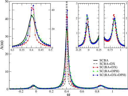
Figure 13: (color online). Non-equilibrium spectral function (bias $V=0.45>\omega_{0}$) for the off-resonant transport regime for the weak/intermediate electron-vibron coupling. Calculations were performed self-consistently with first-order Hartree and Fock-like diagrams (SCBA curve), and with second-order DX and/or DPH diagrams (SC(BA+DX,+DPH,+DX+DPH) curves). Second-order DX correction to SCBA is also shown (SCBA+DX curve). The top-left inset shows a zoom on the central peak around $\omega\sim 0.4$, and the top-right insets show a zoom on the vibron side-band peaks around $\omega\sim 0.0$ and $\omega\sim 0.8$. The other parameters are $\varepsilon_{0}=+0.5$ , $\gamma_{0}=0.2,\omega_{0}=0.4,t_{0L,R}=0.15,\eta=0.025,\eta_{V}=1$. The second-order DX diagram narrows the peaks with a slight shift of the side-band peaks towards the central peak. The narrowing is too strong in the case of partially self-consistent calculations (SCBA+DX). The second-order DPH diagram broadens the peak, but not as much as in the resonant case. Full self-consistent calculations including both second-order diagrams result in an intermediate behaviour for the modifications of the spectral functions.

III.4.4 Resonant regime at finite bias

As we have already shown in the first-order electron-vibron diagrammatic calculations, the spectral functions for the off-resonant and resonant regime at non-equilibrium are qualitatively similar, in the sense that they present a central peak with vibron side-band peaks on both sides. One can compare for example the spectral functions obtained for Hartree-Fock-like calculations at non-equilibrium shown in Figure 6 and Figure 8.

Hence, and again on a qualitative level, the effects of the second-order DX and DPH diagrams on the resonant case at finite bias are similar to what has been obtained for the off-resonant non-equilibrium case described in the previous section. The effects of these higher-order diagrams on the full non-equilibrium transport properties for the different transport regimes will be presented in a forthcoming paper.

However before turning the discussion to the linear-response properties of the system at and near equilibrium, we would like to comment on a specific aspect of the effects of higher-order diagrams.

The narrowing of the vibron side-band peaks and of the main central peak due to higher-order (DX) diagrams was also obtained by other authors (see for example Ref. [Zazunov and Martin, 2007]). In this paper, a different non-equilibrium approach was used. It consists of starting with an electron dressed by a vibron (a polaron) in the isolated central region, then using perturbation expansion theory (with partial resummation) in terms of the coupling of the central region to the non-equilibrium left and right leads. However, the results for the spectral functions in Ref. [Zazunov and Martin, 2007] were only given for the resonant transport regime at equilibrium and all calculations were performed without the Hartree-like diagram. Though we have already shown that such a diagram plays a crucial role in the spectral properties of the system in the resonant regime at and out of equilibrium.

III.5 Linear response transport properties

We now briefly discuss the effects of electron-vibron interaction taken at different levels of the diagrammatic expansion on the linear-response transport properties of the single-molecule nanojunction. Before doing so, we explain how to derive the linear conductance from the value of the spectral functions calculated at equilibrium.

In our model, there is a direct proportionality between the left and right leads’ self-energies $\Sigma^{r}_{L,R}$ because, the central region is coupled to the leads via the single hopping matrix element and we have chosen identical leads. Then the current (Eq. (20)) can be recast as follows (for the details of the derivation, see for example Refs.[Meir and Wingreen, 1992; Ness, 2006]):

$$I=-4e/h\int{\rm d}\omega\left(f_{L}(\omega)-f_{R}(\omega)\right)\Gamma(\omega)\Im m[G^{r}(\omega)],$$ (30)

where $\Gamma=\Gamma_{L}\Gamma_{R}/(\Gamma_{L}+\Gamma_{R})$ and $\Gamma_{\alpha}=-2\Im m[\Sigma^{r}_{\alpha}]$.

The linear conductance

$$G_{\rm lin}=\frac{dI}{dV}|_{V\rightarrow 0}$$

is obtained from

$$G_{\rm lin}/G_{0}=-2\Gamma(\mu^{\rm eq})\ \Im m[G^{r}(\mu^{\rm eq})]=2\Gamma(\mu^{\rm eq})\ A(\mu^{\rm eq})$$ (31)

where $G_{0}=2e^{2}/h$ is the quantum of conductance.

Table 1 shows the different values for the linear conductance $G_{\rm lin}$ obtained from the equilibrium spectral functions shown in figures 10, 11 and 12.

$G_{\rm lin}/G_{0}$	off-resonant	off-resonant	resonant
	weak e-vib	strong e-vib	(e-h symmetric)
	Fig. 10	Fig. 11	Fig. 12
SCBA	0.002654	0.004470	0.8379∗
SCBA+DX	0.002666	0.004606	-
SCBA+DX+DPH	0.003186	-	-
SC(BA+DX)	0.002668	0.004606	1.1296
SC(BA+DPH)	-	-	0.7194
SC(BA+DX+DPH)	-	0.004638	0.8545
MCIST	0.002621	0.004936	n.a.
no e-vib	0.002021	0.002021	1.

^∗ in principle here $G_{\rm lin}$ should be $G_{0}$ but is not because we are using a tiny but finite $\eta=0.030$ value. See appendix B for detailed explanations.

Table 1: Linear conductance $G_{\rm lin}={dI}/{dV}|_{V\rightarrow 0}$ obtained from the value of the equilibrium spectral density at $\omega=\mu^{\rm eq}$. $G_{\rm lin}$ is given in units of the quantum of conductance $G_{0}=2e^{2}/h$. The equilibrium spectral functions are shown in Figs.  10,  11 and  12) and were done for different different levels of approximation as explained in the corresponding figure captions.

For the off-resonant regime at the weak electron-vibron coupling, there are not many differences in the linear conductance $G_{\rm lin}$ values calculated for all the different diagrams, as one might expect from the spectral function behaviour shown in figure 10. This is especially true when the main peak in the spectral function is located well away from the Fermi level, i.e. $|\tilde{\epsilon}_{0}-\mu^{\rm eq}|\gg$ linewidth of the peaks. For strong electron-vibron coupling, the differences between different levels of approximations are more pronounced. All $G_{\rm lin}$ values are smaller than the exact MCIST result. This is essentially due to the fact that perturbation expansion gives only an approximate value of the polaron shift. The differences from the exact result are more important for SCBA-based calculations (difference of $\sim 10\%$ with exact result) and of course calculations performed up to second order give a better polaron shift and hence better values for the linear conductance ($\sim 5\%$ difference only).

In the quasi-resonant case when $|\tilde{\epsilon}_{0}-\mu^{\rm eq}|\sim$ (1 to 2) linewidth, the effects described above will be more pronounced, because the linear conductance is no longer given by the extreme tail of the main peak crossing the Fermi level.

For the resonant case in the absence of the Hartree potential, the SCBA-based calculations should give a perfect linear conductance. The reason why $G_{\rm lin}\neq G_{0}$ is because the calculations were performed with a tiny but finite value of $\eta$ as explained in detail in Appendix B. Hence one may say that, for the chosen set of parameters, the value $G_{\rm lin}=0.838$ represents an upper bound for the linear conductance (the corresponding numerical perfect conductance). And as explained in Appendix B, linear conductance values can only be compared between calculations performed with the same value of $\eta$, which is what we have done.

The linear conductance is strongly renormalized (decreased and increased) when including only one of the two second-order diagrams (DPH and DX respectively). In contrast, it becomes close again to the expected quantum of conductance when the calculations are performed with both second-order diagrams. This dependence of the conductance is well understood from the behaviour of the spectral functions shown in Figure 12. SC(BA+DPH) calculations introduce an extra broadening and a corresponding decrease of amplitude of the peaks in the spectral functions, hence a decrease of $G_{\rm lin}$. However, the strong narrowing, with increased amplitude, of the peaks due to SC(BA+DX) calculations leads to an increase of $G_{\rm lin}$. The SC(BA+DX) calculations give a linear conductance larger than that obtained from SCBA, i.e. $G_{\rm lin}>G_{0}$, which is an unphysical result for our non-degenerate electronic level in the central part of the system.

This implies a strong constraint on the validity of the values of $G_{\rm lin}$ obtained from a many-body perturbation expansion: in order to conserve the Fermi-liquid properties (see Appendix B) in the electron-hole symmetric resonant regime, one has to perform the calculations by including all diagrams order by order. Results obtained from partial resummation of a subset of diagrams will probably give an incorrect linear conductance.

Hence calculations performed by fully renormalizing the vibron propagators Galperin et al. (2004a); Viljas et al. (2005) or all crossing diagrams Zazunov and Martin (2007), while containing diagrams higher than second order, will probably break important physical properties of the system at $T=0$, because they lack important electronic processes, to second-order the DX vertex correction-like diagram or DPH diagram respectivelly.

In the resonant (or quasi-resonant) regime, polarisation effects and vertex corrections play an equally important role in the electronic structure and transport properties of electron-vibron interacting nanojunctions which electron-hole symmetry.

IV Conclusion

In this paper, we have presented a method based on NEGF to calculate the equilibrium and non-equilibrium electronic structure of electron-vibron interacting single-molecule junctions. We have applied the method to a model system which consists of a single electronic level coupled to a single vibration mode in the central region, the latter in contact with two non-equilibrium electron reservoirs.

In comparison to previous studies performed within a similar approach Mii et al. (2003); Frederiksen et al. (2004); Galperin et al. (2004b); Mitra et al. (2004); Pecchia and di Carlo (2004); Chen et al. (2005b); Ryndyk and Keller (2005); Sergueev et al. (2005); Viljas et al. (2005); Yamamoto et al. (2005); Cresti et al. (2006); de la Vega et al. (2006); Egger and Gogolin (2008), the novelty of our method lies in the fact that it goes beyond the conventionally-used self-consistent Born approximation (SCBA). Higher-order diagrams for the electron-vibron interacting have been implemented in our calculations.

In this paper we have considered the second-order diagrams which contain two-vibron processes: the so-called double exchange DX diagram which is part of the vertex corrections to SCBA, and the partially dressed DPH diagram in which the vibron propagator is renormalized by one electron-hole bubble.

We have studied the effects of the first and second-order diagrams on the spectral functions for a large set of parameters and for different transport regimes (resonant and off-resonant cases) at equilibrium and in the presence of a finite applied bias driving the system out of equilibrium.

We have shown the important role played by the Hartree diagram in calculations based only on first-order diagrams. Such a diagram should not be neglected unless one works within an applied bias range for which the correspond Hartree potential is constant.

For calculations including both first and second-order diagram we have found that the effects of the individual second-order diagram are as follows: the DX diagram reduces the width of the peaks in the spectral functions, with an increase of their height, while the DPH has the opposite effect: it increases the width and decreases the height. Furthermore, the DX diagram moves the vibron side-band peak position towards the main peak, and hence gives a better peak separation as should be obtained from exact calculations. Calculations performed with both DX and DPH diagram give intermediate results for the spectral functions, which are not simply an average/superposition of the individual effects because of the strong non-linearity involved in solving the problem self-consistently.

Furthermore, the effects of the second-order diagrams also depend on the transport regime: at and near equilibrium, the DX diagram dominates over the DPH diagram in the off-resonant transport regime (essentially because there are not many electron-hole excitations available in this regime). In the resonant case, however, both DX and DPH play an equally important role. For large non-equilibrium conditions ($V>\omega$), both second-order diagrams play an important role, since the corresponding spectral functions look qualitatively similar to those obtained the resonant regime.

We have thus shown that it is indeed necessary to go beyond SCBA to obtain the correct results for a wide range of parameters. This has also been confirmed by comparing our NEGF results to an exact calculation in terms of electron-vibron interacting (the multi-channel inelastic scattering technique MCIST Ness (2006)), though it should be noted that comparison between NEGF and MCIST calculations are only valid for the off-resonant transport regime.

We have also studied in detail the effects of self-consistency on the calculations, especially for the cases including the second-order diagrams (see Section III.4.1 and Figure 11). We have found a solution to an old problem, well known in many-body perturbation theory: in order to avoid negative spectral densities when including higher order diagrams in the calculations, it seems more appropriate to start the self-consistent loop with SCBA (Hartree-Fock like) electron Green’s functions .

Finally, we have studied the linear response (linear conductance $G_{\rm lin}$) of the nanojunctions, and have found that in the off-resonant regime, the value of $G_{\rm lin}$ is governed by the behaviour of the tail of the main peak at the Fermi level, hence it depends on both the position and the width of this peak. In the off-resonant regime, the DPH diagram contribution is negligible and the DX diagram gives a better polaron shift (better position of the main peak) and hence the second-order (mostly DX) calculation gives a better agreement for $G_{\rm lin}$ with the exact result. For the near-resonant regime, the contribution of DPH will become more important and both DX and DPH will play an important role in determining the value of $G_{\rm lin}$ by changing both the position and the width of the main peak.

For the resonant regime with electron-hole symmetry, it is necessary to perform the calculations by including both DX and DPH diagrams in order to conserve the Fermi-liquid properties of the system. We anticipate that this will be also true for higher-order diagrams and calculations need to be performed by including all diagrams of the same order. Calculations performed with partial resummation of a subset of diagrams will break the expected Fermi-liquid properties of the system and will probably lead to an incorrect value of the linear conductance.

Finally, we expect that the effects of the second-order diagrams, shown in this paper for the spectral functions only, are also important in the full non-equilibrium transport properties of the nanojunctions. The study of these effects on the non-linear conductance are currently undertaken and will be considered in a forthcoming paper.

Appendix A Self-energies for the Born approximation and the second-order diagrams

In this appendix, we show how to derive the expression for the self-energies corresponding to one- and two-vibron process diagrams in terms of electron-vibron coupling.

Starting from the SSSM Hamiltonian, the general definition of the one-particle GF of the central region is obtained from the time-loop contour-ordered product of the creation and annihilation operators in the central region

$$G(\tau,\tau^{\prime})=-{\rm i}\langle T_{C_{K}}d_{H}(\tau)d^{\dagger}_{H}(\tau^{\prime})\rangle.$$ (32)

The time-loop contour $C_{K}$ contains two branches, the upper $(+)$ and the lower $(-)$ branch. On the upper branch, time starts in the infinitely remote past and evolves forwards, then at the turning point, which can be placed at any arbitrary time, one passes onto the lower branch where the system evolves backwards in time back to the initially non-interacting starting point at $t=-\infty$.

Then any expectation value of products of operator reduces to $\langle\phi_{0}|T_{C_{K}}\left(\hat{A}(\tau)\hat{B}(\tau^{\prime})\dots S_{C_{K}}\right)|\phi_{0}\rangle$ where $\langle\phi_{0}|\dots|\phi_{0}\rangle$ is the average over the non-interacting ground state. The operators are then given in the interaction picture, and $S_{C_{K}}$ is the generalization of the time evolution operator on the Keldysh contour $S_{C_{K}}=T_{C_{K}}\left(\exp\{-{\rm i}\int_{C_{K}}{\rm d}\tau\ \hat{V}(\tau)\}\right)$ where $T_{C_{K}}$ is the time-ordering operator on the contour $C_{K}$ and $\int_{C_{K}}{\rm d}t$ implies integration over $C_{K}$. And $\hat{V}$ is the “perturbation” to the reference Hamiltonian, which in our case would be the interaction electron-vibron as well as the coupling of the central region to the leads).

Expanding $S_{C_{K}}$ as a series in terms of the electron-vibron coupling Hamiltonian $H_{e\text{-vib}}$, one can derive the electron-vibron self-energies to any order of the electron-vibron coupling by calculating any time ordered products in the series using the usual rules of many-body perturbation theory, such as Feynmann diagrammatic expansion or Wick’s theoremMahan (1990); Abrikosov et al. (1963); Fetter and Walecka (1971).

A.1 Lowest order self-energies

The one-vibron process self-energies, corresponding to the Hartree and Fock-like diagrams (see Figure 2) are given by

$$\Sigma^{H}_{e\text{-vib}}(\tau_{1},\tau_{2})=-{\rm i}\gamma_{0}^{2}\ D_{0}(\tau_{1},\tau_{2})\ G(\tau_{1},\tau_{1}^{+})\ ,$$ (33)

and

$$\Sigma^{F}_{e\text{-vib}}(\tau_{1},\tau_{2})={\rm i}\gamma_{0}^{2}\ D_{0}(\tau_{1},\tau_{2})\ G(\tau_{1},\tau_{2})\ ,$$ (34)

where $\tau_{i}$ are times on the time-loop contour.

The projections onto the real (physical) times are given by, for example,

$$\Sigma^{F,\zeta_{1}\zeta_{2}}_{e\text{-vib}}(t_{1},t_{2})={\rm i}\gamma_{0}^{2}\ D_{0}^{\zeta_{1}\zeta_{2}}(t_{1},t_{2})\ G^{\zeta_{1}\zeta_{2}}(t_{1},t_{2})\ ,$$ (35)

for the Fock self-energy .

The index $\zeta_{i}=\pm$ labels the branch of the time-loop contour corresponding to the forward ($\zeta_{i}=+$)/ backward ($\zeta_{i}=-$) time evolution respectively.

There are several useful relationships between the different projections (or Keldysh components) of the Green’s functions $X\equiv G,D$: Keldysh (1965); Craig (1968); Meir and Wingreen (1992); van Leeuwen et al. (2006); Rammer (2007). They are

$$X^{r}=X^{++}-X^{+-}=X^{-+}-X^{--}$$ (36)

or equivalently in terms of time-ordered ($t=++$), anti time-ordered ($\tilde{t}=--$), greater ($>=-+$) and lesser ($<=+-$) Green’s functions:

$$X^{r}=X^{t}-X^{<}=X^{>}-X^{\tilde{t}}$$ (37)

and

$$X^{a}=X^{++}-X^{-+}=X^{+-}-X^{--}$$ (38)

(or equivalently $X^{a}=X^{t}-X^{>}=X^{<}-X^{\tilde{t}}$), and hence $X^{r}-X^{a}=X^{>}-X^{<}$.

Similar relationships exist for the self-energies $\Sigma^{x}\leftrightarrow X^{x}$ ($x=r,a,<,>,t,\tilde{t}$).

Using these relationships and taking the steady state limit, i.e. $X(t,t^{\prime})=X(t-t^{\prime})$, and after Fourier transformation into an energy representation $X(\omega)$, we obtain the usual expressions Mii et al. (2003); Frederiksen et al. (2004); Galperin et al. (2004a); Mitra et al. (2004); Pecchia et al. (2004); Chen et al. (2005b); Ryndyk and Keller (2005); Sergueev et al. (2005); Viljas et al. (2005); Yamamoto et al. (2005); Cresti et al. (2006); de la Vega et al. (2006); Egger and Gogolin (2008) for the Hartree $\Sigma^{H,x}_{e\text{-vib}}(\omega)$ and Fock $\Sigma^{F,x}_{e\text{-vib}}(\omega)$ electron-vibron self-energies ($x=r,a,<,>$).

For example, the Hartree and Fock self-energies are

$$\Sigma^{H,x}_{e\text{-vib}}(\omega)=-{\rm i}\gamma_{0}^{2}\ D_{0}^{x}(\omega=0)\ \int\frac{{\rm d}\omega^{\prime}}{2\pi}\ G^{<}(\omega^{\prime})\ ,$$ (39)

$$\Sigma_{{e\text{-vib}}}^{F,y}(\omega)=i\gamma_{0}^{2}\int\frac{d\omega^{\prime}}{2\pi}\ D_{0}^{y}(\omega^{\prime})\ G^{y}(\omega-\omega^{\prime})\ ,$$ (40)

where $y$ represents one of the tree Keldysh compoentns $y=t,<,>$. Using the relationship $\Sigma^{r}=\Sigma^{t}-\Sigma^{<}$, we find

$$\Sigma_{e\text{-vib}}^{F,r}(\omega)={\rm i}\gamma_{0}^{2}\int\frac{d\omega^{\prime}}{2\pi}D_{0}^{r}(\omega-\omega^{\prime})G^{<}(\omega^{\prime})\hfill\\ \qquad+D_{0}^{<}(\omega-\omega^{\prime})G^{r}(\omega^{\prime})+D_{0}^{r}(\omega-\omega^{\prime})G^{r}(\omega)\ .\\$$ (41)

With the usual definitions for the bare vibron Green’s functions $D_{0}$:

$$\begin{split}D_{0}^{<}(\omega)&=-2\pi i\left[\langle N_{\text{ph}}\rangle\delta(\omega-\omega_{0})\right.\\ &\qquad\left.+(\langle N_{\text{ph}}\rangle+1)\delta(\omega+\omega_{0})\right],\end{split}$$ (42)

$$\begin{split}D_{0}^{>}(\omega)&=-2\pi i\left[\langle N_{\text{ph}}\rangle\delta(\omega+\omega_{0})\right.\\ &\qquad\left.+(\langle N_{\text{ph}}\rangle+1)\delta(\omega-\omega_{0})\right],\end{split}$$ (43)

$$\begin{split}D_{0}^{r}(\omega)&=\frac{1}{\omega-\omega_{0}+i\eta}\\ &\qquad-\frac{1}{\omega+\omega_{0}+i\eta},\quad\eta\rightarrow 0^{+}\end{split}$$ (44)

$$D_{0}^{a}(\omega)=[D_{0}^{r}(\omega)]^{*},$$ (45)

where $\langle N_{\text{ph}}\rangle$ is the averaged number of excitations in the vibration mode of frequency $\omega_{0}$ given by the Bose-Einstein distribution at temperature $T_{\rm vib}$.

One can see that $\Sigma^{H,<,>}_{e\text{-vib}}(\omega)=0$ because $D_{0}^{<,>}(\omega=0)=0$ unless $\omega_{0}=0$ which would be an odd case of study. And since $D_{0}^{r,a}(\omega=0)=-2/\omega_{0}$, one has

$$\Sigma_{e\text{-vib}}^{H,r}=\Sigma_{e\text{-vib}}^{H,a}=\frac{\gamma_{0}^{2}}{\omega_{0}}2{\rm i}\int\frac{d\omega^{\prime}}{2\pi}G^{<}(\omega^{\prime})\ .$$ (46)

Furthermore the lesser and greater Fock self-energies can be expressed in a more compact form:

$$\begin{split}\Sigma_{{e\text{-vib}}}^{F,\{<,>\}}(\omega)&=\gamma_{0}^{2}\left[\langle N_{\text{ph}}\rangle G^{\{<,>\}}(\omega\mp\omega_{0})\right.\\ &\quad\left.+(\langle N_{\text{ph}}\rangle+1)G^{\{<,>\}}(\omega\pm\omega_{0})\right].\end{split}$$ (47)

A.2 Second-order self-energies

The two-vibron process self-energies correspond to the two diagrams shown in Figure 3, i.e. the so-called double exchange (DX) diagram and GW-like (dressed phonon/vibron DPH) diagram in which the vibron propagator is renormalized by a single electron-hole bubble polarization.

The expressions for the self-energies for these diagrams are:

$$\begin{split}\Sigma^{DX}_{e\text{-vib}}(\tau_{1},\tau_{2})=-\frac{\gamma_{0}^{4}}{3}\int_{C_{K}}&{\rm d}\tau_{3}{\rm d}\tau_{4}G(\tau_{1},\tau_{3})D_{0}(\tau_{1},\tau_{4})\times\\ &G(\tau_{3},\tau_{4})D_{0}(\tau_{3},\tau_{2})G(\tau_{4},\tau_{2}),\end{split}$$ (48)

and

$$\begin{split}\Sigma^{DPH}_{e\text{-vib}}(\tau_{1},\tau_{2})=+\frac{\gamma_{0}^{4}}{3}G(\tau_{1},\tau_{2})\times\\ \int_{C_{K}}{\rm d}\tau_{3}{\rm d}\tau_{4}D_{0}(\tau_{1},\tau_{3})G(\tau_{3},\tau_{4})G(\tau_{4},\tau_{3})D_{0}(\tau_{3},\tau_{2}).\end{split}$$ (49)

The factor $1/3$ comes from the series expansion of the exponential in the time evolution operator $S_{C_{K}}$ and the fact that one obtains 8 equivalent diagrams of the $\gamma_{0}^{4}$ order.

Taking the steady state limit and after Fourier transformation, the different Keldysh components of the double-exchange (DX) self-energy are given by

$$\begin{split}\Sigma^{DX,\zeta_{1}\zeta_{2}}_{e\text{-vib}}(\omega)=-\frac{\gamma_{0}^{4}}{3}\int\frac{{\rm d}u}{2\pi}\frac{{\rm d}v}{2\pi}\sum_{\zeta_{3},\zeta_{4}}\zeta_{3}\zeta_{4}G^{\zeta_{1}\zeta_{3}}(v)\times\\ D_{0}^{\zeta_{i}\zeta_{4}}(\omega-v)G^{\zeta_{3}\zeta_{4}}(v-u)D_{0}^{\zeta_{3}\zeta_{2}}(u)G^{\zeta_{4}\zeta_{2}}(\omega-u).\end{split}$$ (50)

A.3 Normalisation of the vibron propagators

The expression for the self-energy $\Sigma^{DPH}_{e\text{-vib}}(\tau_{1},\tau_{2})$ can actually be recast in a Fock-like diagram with a renormalised vibron propagator $\mathcal{D}_{0}$ Galperin et al. (2004a); Viljas et al. (2005):

$$\Sigma^{F}_{e\text{-vib}}(\tau_{1},\tau_{2})={\rm i}\gamma_{0}^{2}\ \mathcal{D}_{0}(\tau_{1},\tau_{2})\ G(\tau_{1},\tau_{2})\ ,$$ (51)

where the dressed vibron $\mathcal{D}_{0}(\tau,\tau^{\prime})$ is given by

$$\mathcal{D}_{0}(\tau,\tau^{\prime})=\gamma_{0}^{2}\ \int_{C_{K}}{\rm d}\tau_{2}{\rm d}\tau_{3}\ D_{0}(\tau,\tau_{3})\ \Pi(\tau_{3},\tau_{2})\ D_{0}(\tau_{2},\tau^{\prime})$$ (52)

and the polarization $\Pi(\tau,\tau^{\prime})$ is given by the electron-hole bubble diagram:

$$\Pi(\tau,\tau^{\prime})=-{\rm i}\ G(\tau,\tau^{\prime})\ G(\tau^{\prime},\tau)\ .$$ (53)

So, in principle, we already have all the ingredients to perform calculations using the fully dressed vibron propagator $\mathcal{D}(\omega)$ Galperin et al. (2004a); Viljas et al. (2005) whose advanced and retarded components are given by

$$\mathcal{D}^{\{r,a\}}(\omega)=\left[[D_{0}^{\{r,a\}}(\omega)]^{-1}-\gamma_{0}^{2}\ \Pi^{\{r,a\}}(\omega)\right]^{-1}\ .$$ (54)

The vibron spectrum is renormalized by the polarization. Ther is a shift of the vibron energy related to $\gamma_{0}^{2}\Re e\Pi^{\{r,a\}}$ and a finite linewidth of the peaks related to $\gamma_{0}^{2}\Im m\Pi^{\{r,a\}}$, instead of Dirac $\delta$ peaks as in Eq.(55).

We have not performed the full vibron renormalization in the present work, because we want to study the effects of different diagrams of the same order, and order by order. $\mathcal{D}(\omega)$ correspond to a partial resummation of all the bubble diagrams and contains all (even) orders of the electron-vibron coupling. The effect of this GW-like electron-vibron interaction will be presented in a forthcoming paper.

Appendix B Details of numerical calculations

In this section we provide more details about how calculations for the self-energies are performed.

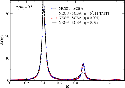
Figure 14: Equilibrium spectral functions for the off-resonant regime calculated with MCIST and NEGF-SCBA. MCIST calculations are performed at the Hartree-Fock level (BA). NEGF are done using the limit $\eta\rightarrow 0^{+}$ for the imaginary part of the bare vibron GF and also by using a tiny, but finite value for $\eta$ (0.001 and 0.025). See main text for details. The other parameters are $\varepsilon_{0}=+0.5$ (electron transport), $\gamma_{0}=0.20$ (upper panel), $\omega_{0}=0.40,t_{0L}=t_{0R}=0.15$. For a small enough value of $\eta$, one recovers the exact MCIST as well as the $\eta\rightarrow 0^{+}$ NEGF results obtained from Hilbert transform (HT). Larger values of $\eta$ widen the peaks; however the spectroscopic information remains. For such values of $\eta$, one can work with fewer grid points and makes second-order self-energy calculations tractable.

First, we start by using the following decomposition of the retarded and advanced vibron propagator $D_{0}^{r,a}$:

$$\begin{split}D_{0}^{r,a}(\omega)&=\frac{1}{\omega-\omega_{0}\pm{\rm i}\eta}-\frac{1}{\omega+\omega_{0}\pm{\rm i}\eta},\quad\eta\rightarrow 0^{+}\\ &=\mathrm{P.V.}\frac{1}{\omega-\omega_{0}}-\mathrm{P.V.}\frac{1}{\omega+\omega_{0}}\\ &\qquad\mp i\pi(\delta(\omega-\omega_{0})-\delta(\omega+\omega_{0}),\end{split}$$ (55)

and the definition of the Hilbert transformation (H.T.):

$$\mathcal{H}(y)=\mathrm{H.T.}[f(x)]=\frac{1}{\pi}\mathrm{P.V.}\int_{-\infty}^{\infty}dx\frac{f(x)}{x-y}.$$ (56)

One can then rewrite the Fock retarded (advanced) self-energy in terms of retarded (advanced) and lesser electron Green’s functions only:

$$\begin{split}\Sigma_{e\text{-vib}}^{F,r}(\omega)=&\gamma_{0}^{2}\biggl{[}\langle N_{\text{ph}}\rangle G^{r}(\omega-\omega_{0})+(\langle N_{\text{ph}}\rangle+1)G^{r}(\omega+\omega_{0})+\frac{1}{2}\left(G^{<}(\omega-\omega_{0})+G^{r}(\omega-\omega_{0})-G^{<}(\omega+\omega_{0})-G^{r}(\omega+\omega_{0})\right)\\ &\quad+\frac{i}{2}\left(\mathcal{H}[G^{<}+G^{r}](\omega+\omega_{0})-\mathcal{H}[G^{<}+G^{r}](\omega-\omega_{0})\right)\biggr{]},\end{split}$$ (57)

and

$$\begin{split}\Sigma_{e\text{-vib}}^{F,a}(\omega)=&\gamma_{0}^{2}\biggl{[}\langle N_{\text{ph}}\rangle G^{a}(\omega-\omega_{0})+(\langle N_{\text{ph}}\rangle+1)G^{a}(\omega+\omega_{0})-\frac{1}{2}\left(G^{<}(\omega-\omega_{0})-G^{a}(\omega-\omega_{0})-G^{<}(\omega+\omega_{0})+G^{a}(\omega+\omega_{0})\right)\\ &\quad+\frac{i}{2}\left(\mathcal{H}[G^{<}-G^{a}](\omega+\omega_{0})-\mathcal{H}[G^{<}-G^{a}](\omega-\omega_{0})\right)\biggr{]}.\end{split}$$ (58)

These expressions are in a form convenient for computation, since, as for $\Sigma_{e\text{-vib}}^{F,<,>}$, they involve the direct evaluation of $G^{r,a,<}$ on a energy grid shifted by $\pm\omega_{0}$ in addition with the Hilbert transform of $G^{<}$ and $G^{r,a}$ on a shifted energy grid.

The Hilbert transformation is actually a conventional convolution product of the trial function with an appropriate $(1/x)$-like kernel. Calculation of convolution products can be made faster, instead of scaling as the square of the number of grid points, by the use of FFT routines. However since FFT routines introduce artifical periodic boundary conditions, and one has to make sure that the functions, which decay slowly as $1/\omega$ (the kernel of the Hilbert transform, and real part of $G^{r,a}$), have sufficiently small values at the boundaries of the energy grid. Otherwise, the corresponding discontinuities introduce spurious oscillations in the FFT. This means that one has to work with a wide energy grid and with a correspondingly large number of grid points to keep a good enough resolution.

Working with a large number of grid points $N_{\rm pts}>10^{4}$ is not really a problem when calculating convolution products with FFT, since the number of operations reduces from $N_{\rm pts}^{2}$ to $N_{\rm pts}\log_{2}N_{\rm pts}$, or even when without using FFT routines. However, it is not possible to reduce the calculation of the second-order DX self-energy to some sort of convolution product, and the number of operations then scales as $N_{\rm pts}^{3}$. Such a scaling starts to make calculations seriously impractical when working with a large number of grid points.

Hence, we have adopted another stategy which consists of introducing, in the definition of $D_{0}^{r,a}$, a tiny but finite imaginary part $\rm i\eta$ instead of taking the limit $\eta\rightarrow 0^{+}$. This is just a natural step towards working with a fully dressed (renormalized) vibron propagator as already discussed in Section A.3.

By using this tiny but finite imaginary part $\rm i\eta$, we avoid having to deal numerically with the Dirac $\delta$-function and consequently with the Hilbert transform and all the problems associated with the slowly decaying kernel. We can then work with a less wide energy grid and fewer points while keeping a good energy resolution. Hence the calculations of the second order DX self-energy become more tractable. Of course, there is a price to pay for that: there is a lowest bound for the possible values of $\eta$, and this lowest bound is strongly linked to the value of the grid spacing. By trial and error, we have found that $\eta$ must be at least equal to 2 or 3 times the grid spacing.

Now we have to check and compare the results for the spectral functions obtained from these two different methods of calculation. Figure 14 show the spectral functions for the off-resonant regime at equilibrium and for weak/intermediate electron-vibron coupling. Calculations have been performed with MCIST at the Hartree-Fock level (MCIST-SCBA) which serves as a reference calculation. The NEGF-SCBA calculations performed within the limit $\eta\rightarrow 0^{+}$ by using Hilbert transform and FFT for the Fock self-energy (in the present case with a 131072 grid points ranging from -30 to +30) are identical to the MCIST-SCBA results as expected. The NEGF-SCBA calculations performed with a tiny but finite imaginary part $\rm i\eta$ have been done for different sets of parameters. Only two are shown in Figure 14: $\eta=0.001$ corresponding to a energy grid ranging from -10 to +10 and with 32769 points, and $\eta=0.025$ corresponding to a energy grid ranging from -10 to +10 and with 2049 points. The spectral function obtained with $\eta=0.001$ is virtually identical to the corresponding “exact” calculations, while the spectral function obtained with $\eta=0.025$ has slightly broadened peaks with a reduced amplitude, even though such a calculation has been performed with only 2049 grid points—which is in the range of good values of grid points to make calculation of the second-order DX self-energy numerically tractable. In any case, the most important point is that the spectral information (peak positions) are not dependent on the finite value of $\eta$.

Now we also have to verify the influence of $\eta$ on another transport regime for which we do not have any exact reference calculations, but for which we may expect to recover conventional properties of an interacting Fermi liquid at very low temperatures.

Figure 15 shows the equilibrium spectral functions for the resonant regime. Calculations are performed with only the Fock self-energy and for different values of $\eta$ (0.03, 0.01875, 0.00938, 0.001875, 0.000938) and for different number of energy grid points (2049, 32769, 65537, 131073). The energy grid is ranges from -10 to +10. As expected, the main central peak and the vibron side-band peak narrow with increasing amplitude when the value of $\eta$ decreases, until reaching an asymptotic behaviour for $\eta\sim 10^{-3}$.

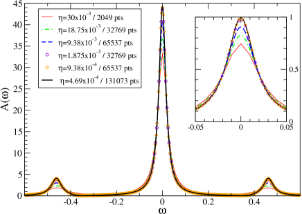
Figure 15: (Color online). Equilibrium spectral functions for the resonant regime obtained within NEGF (Fock self-energy only). Calculations are performed for different values of the imaginary part $\eta$ (0.03, 0.01875, 0.00938, 0.001875, 0.000938) and for different number of energy grid points (2049, 32769, 65537, 131073). The energy grid is ranging from -10 to +10. The inset shows a zoom around $\omega=0$ of the rescaled spectral functions, giving then the linear conductance $G_{\rm lin}$ at $\omega=0$. The other parameters are $\varepsilon_{0}=0.0$, $\gamma_{0}=0.23$ , $\omega_{0}=0.40,t_{0L}=t_{0R}=0.15$. Peaks in the spectral functions narrow with decreasing values of $\eta$ as expected. And one recovers a perfect linear conductance $G_{\rm lin}=G_{0}$ at $T=0$.

The most interesting result is given by the behaviour of spectral function at the equilibrium Fermi level $\mu^{\rm eq}=0$. Such a behaviour is exemplified in the inset of Figure 15. The inset shows the spectral function rescaled by $2\Gamma(\mu^{\rm eq})$ so that the value at $\omega=0$ corresponds to the linear conductance $G_{\rm lin}$ (see Section III.5). One can see that $G_{\rm lin}$ goes towards the unit of conductance as $\eta\rightarrow 0$. Such a limit corresponds to a perfect conductance, as obtained for the corresponding non-interacting system.

This result shows that even in the presence of electron-vibron interactions, the linear conductance is perfect, as one also obtains for the non-interacting case. The electron-vibron interaction (as least at the Fock level) does not renormalize the linear conductance. For the fully electron-hole symmetric system (no Hartree self-energy), we have checked that the value of $\Im m\Sigma^{r}_{e\text{-vib}}(\omega)$ is zero at $\omega=0$ and at $T=0$ (at equilibrium). The real part of the interacting self-energy $\Re e\Sigma^{r}_{e\text{-vib}}=0$ at $\omega=0$ by definition because it is an odd function of $\omega$. Our electron-vibron interacting system conserves its Fermi-liquid properties at zero temperature and equilibrium, as also obtained for interacting electron systems (see for example Refs.[Ferretti et al., 2005a, b; Cornaglia et al., 2004; Oguri, 1997]). We expect that such a behaviour also hold for other electron-vibron diagrams than the Fock diagram. Out of equilibrium, the system may lose its conventional Fermi-liquid properties, as we have already shown in the main part of the paper.

In conclusion, we want to stress that by introducing a finite, but tiny, value for the imaginary part $\eta$, one might not get the exact linear conductance value. However this is a numerical artifact which can be controlled by increasing the number of energy grip points and reducing the value of $\eta$. Nonetheless we expect that the relative effects of different electron-vibron diagram are correctly obtained from our calculations, whatever the small values of $\eta$ are. And of course, in order to perform a correct analysis of such effects, one should only compare results for either spectral functions or linear conductance obtained numerically with the same value of $\eta$.