HCN emission from the H ii regions G75.78+0.34 and G75.77+0.34

Abstract

We present images for the 3.5 mm continuum and HCN(J=1–0) hyperfine line emission from the surroundings of the H ii regions G75.78+0.34 and G75.77+0.34 obtained with the Berkeley Illinois Maryland Association (BIMA) interferometer using the D configuration at a spatial resolution of $\sim$18 arcsec and spectral sampling of 0.34 km s^-1. The continuum emission of both objects is dominated by free-free emission from the ionized gas surrounding the exciting stars. Dust emission may contribute only a small fraction of the 3.5 mm continuum from G75.78+0.34 and is negligible for G75.77+0.34. The high spectral resolution reached by BIMA allowed us to separate the emission from each hyperfine transition (F=1-1, F=2-1 and F=0-1), as well as to construct velocity channel maps along each emission-line profile. The HCN flux distributions are similar to those observed for the CO emission, but with some knots of high intensities indicating that the HCN traces high density clouds not seen in CO. The HCN hyperfine line ratios for both H ii regions differ from those predicted theoretically for Local Thermodynamic Equilibrium (LTE), probably due to scattering of radiation processes. The velocity channels shows that the HCN emission of G75.78+0.34 follows the bipolar molecular outflows previously observed in CO. For G75.77+0.34, the outflowing gas contributes only a small fraction of the HCN emission.

1 Introduction

H ii regions are among the most well-studied class of objects of our Galaxy. However most of these studies are based on optical imaging and spectroscopy, in which the earliest stages of the life of stars cannot be accessed. At the early stages, the star(s) and the surrounding H ii region, are still embedded in the molecular cloud which is invisible at optical wavelengths. Nevertheless, they can be observed at longer wavelength, such as radio and infrared bands, which are less affected by extinction than the optical region of the spectra (Wood & Churchwell, 1989; Shepherd, Churchwell & Wilner, 1997; Carral et al., 1997; Franco et al., 2000a; Roman-Lopes et al., 2009).

Usually, according to their sizes, density, mass of ionized gas and emission measure (EM), H ii regions are classified as ultracompact, compact and extended (e.g. Habing & Israel, 1979). Ultracompact H ii regions have sizes of $\lesssim$0.1 pc, display densities of $\gtrsim$10⁴ cm⁻³ , mass of ionized gas of $\sim$10^-2 M_⊙ and EM$\gtrsim$10⁷ pc cm^-6. They are located in the inner, high-pressure, regions of molecular clouds (e.g. Kurtz, Churchwell & Wood, 1994; Franco et al., 2000b). Compact H ii regions have sizes of $\lesssim$0.5 pc, densities $\gtrsim 5\times$10³ cm⁻³, mass of ionized gas of $\sim$1 M_⊙ and EM$\gtrsim$10⁷ pc cm^-6, while classical H ii regions have sizes $\sim$10 pc, densities of $\sim$100 cm⁻³, $\sim$10⁵ M_⊙ of ionized gas and EM$\sim$10² pc cm⁻⁶ (Franco et al., 2000b; Kurtz, 2005). Franco et al. (2000b) present an expansion of this classification including sub-classes and discuss the physical properties of each class (see also Kurtz, 2005, for a review of the physical properties of each class).

The study of the molecular emission close to H ii regions is a key to understand the physical properties of these objects and how stars form. These studies are often based on observations of CO emission for low rotational microwave transitions (e.g. Matthews, Andersson & Mcdonald, 1986; Shepherd & Churchwell, 1996; Shepherd, Churchwell & Wilner, 1997; Qin et al., 2008). The low dipole moment of CO implies that low rotational transitions do not trace dense gas, while molecules with higher dipole moments can be used to observe high density gas. A typical tracer of the emission from dense cores ($n\sim 10^{4}-10^{5}\,{\rm~{}cm^{−3}}$) is the J=1–0 transition from the HCN molecule (e.g. Afonso, Yun & Clemens, 1998).

In this work we present observations of HCN and 3.5 mm continuum images for the H ii regions G75.78+0.34 and G75.77+0.34 obtained with the Berkeley Illinois Maryland Association (BIMA) interferometer. These objects were selected because they present a well-known molecular outflow observed in the CO(J=1–0) emission (Shepherd & Churchwell, 1996; Shepherd, Churchwell & Wilner, 1997), thus being ideal candidates to investigate on whether the high-density gas traced by the HCN has the same distribution and kinematics as the low-density gas traced by CO. These objects are localized in the giant molecular cloud ON2 and were firstly identified by Matthews & Goss (1973) with observations at 5 and 10.7 GHz. These H ii regions are known to be located at a distance of 5.5 kpc (Wood & Churchwell, 1989). G75.77+0.34 presents typical parameters of a compact H ii region and it is excited by an O star, while G75.78+0.34 is at an earlier stage of evolution, being classified as an ultracompact H ii region and is excited by a B star (Matthews & Goss, 1973; Wood & Churchwell, 1989; Shepherd & Churchwell, 1996; Carral et al., 1997; Franco et al., 2000a; Kurtz, 2005). Previous studies of these regions include also the identification of several H₂O maser sources close to the positions of both H ii regions (Hofner & Churchwell, 1996) as well as millimetric radio sources (Carral et al., 1997).

The main goal of this work is to map the distribution and kinematics of the HCN emitting gas from the surroundings of both H ii regions, and compare with those of the CO emitting gas. A secondary goal is to map and discuss the origin of the 3.5 mm radio continuum emission from both regions. In Section 2 we describe the observations and the data reduction. The results for the 3.5 mm continuum and HCN line emission are presented in Section 3, while the discussion of these results are presented in Section 4. Section 5 presents the conclusions of this work.

2 Observations and data reduction

Figure 1: 3.5 mm emission map of G75.78+0.34 and G75.77+0.34 obtained with BIMA at D configuration. The contour levels shown are: $35\times[1,2,3,4,5,6,7,8,9,10]$ mJy.

Interferometric observations of G75.78+0.34 and G75.77+0.34 were obtained with the Berkeley Illinois Maryland Association (BIMA) in June, 1999. A detailed description of the BIMA interferometer can be found in Welch et al. (1996). We used the shortest baseline configuration (D-array), with maximum baseline length of 8900 k$\lambda$, in order to observe the HCN(J=1–0) emission at 88.63 GHz, as well as the 3.5 mm continuum emission.

The primary amplitude and bandpass calibrators were Mars and 3C273, respectively, the latter with a flux density of 22.5 Jy at 3.5 mm. 3C454.3 was also used as a control amplitude calibrator with a derived flux density of 7.2 Jy. An 830-MHz wide continuum channel has been used to produce the 3 mm image, which was strong enough to be used to self-calibrate the visibilities.

The data reduction was performed using standard procedures with the miriad software and included amplitude, phase and bandpass calibrations. The calibrated data has been transported to the aips software for self-calibration and imaging. The resulting full width at half maximum (FWHM) of the synthesized map was about 18 arcsec and the resulting frequency sampling was $\delta\nu\approx 97.656$ kHz for the line emission, corresponding to a velocity sampling of $\delta V\approx 0.34\,{\rm km\,s^{-1}}$.

3 Results

3.1 The 3.5 mm continuum emission

In Figure 1 we present the the 3.5 mm continuum image obtained from the 830-MHz wide channel, which shows that G75.78+0.34 presents a compact circular shape unresolved by our observations, thus corresponding to a linear diameter $\leq$0.5 pc. On the other hand, G75.77+0.34 present a more extended emission which can be described as a “curved” structure with size of about 1^′, corresponding to a linear diameter of $\sim$1.6 pc.

G75.78+0.34 presents a 3.5 mm total flux of $\sim$119 mJy and a peak flux of 92 mJy beam^-1 at the position $\alpha=$20h 21m 43.6s and $\delta=$37^∘ 26^′ 36^′′, approximately coincident with the peak position of higher resolution Very Large Array (VLA) images at 6 cm and 7 mm (Wood & Churchwell, 1989; Carral et al., 1997). The continuum emission for G75.77+0.34 peaks at $\alpha=$20h 21m 41.4s and $\delta=$37^∘ 25^′ 44^′′ with a peak flux density of 352 mJy and a total flux density of $\approx$1.73 Jy. The morphology of the 3.5 mm emission is similar to the 6 cm image presented by Matthews & Goss (1973) at similar spatial resolution.

3.2 The HCN emission

Table 1: Measured fluxes for each transition and flux ratios for G75.78+0.34 and G75.77+0.34. The fluxes are given in Jy and the errors are about 10%. LTE (optically thin) values of $R_{02}$ and $R_{12}$ are 0.2 and 0.6, respectively.

Object	F=1-1	F=2-1	F=0-1	$R_{02}{\rm(F=0-1/F=2-1)}$	$R_{12}{\rm(F=1-1/F=2-1)}$
G75.78+0.34	17.47	14.89	21.25	1.43	1.17
G75.77+0.34	4.39	18.41	11.75	0.64	0.24

The HCN line with angular momentum change from J=1-0 presents three hyperfine transitions at 88.63042 GHz (F=1-1), 88.63185 GHz (F=2-1) and 88.63394 GHz (F=0-1) (see, e.g., Truong-Bach & Nguyen-Q-Rieu, 1989; Afonso, Yun & Clemens, 1998). The high spectral resolution reached by BIMA in D configuration allowed us to separate and construct two-dimensional maps for the flux distribution of each hyperfine transition. The resulting flux contours are shown in Figures 2, 3 and 4, for the transitions F=0-1, F=2-1 and F=1-1, respectively. In order to compare the HCN flux distribution with the 3.5 mm continuum emission we present in these figures the continuum image as a gray scale image. Both axis are shown in arcsec units in order to more easily measure the sizes of the extended emission and the position (0,0) corresponds to the location of the ultracompact H ii region G75.78+0.34. As observed in these figures the HCN emission of G75.78+0.34 for the three hyperfine transitions is spatially coincident with the continuum emission, while for G75.77+0.34 it peaks at $\alpha=$20h 21m 41s and $\delta=$37^∘ 25^′ 24^′′, approximately 25^′′ south-west from the position of the H ii region. In contrast to the continuum emission, the HCN emission is more extended for G75.74+0.34 than for G75.77+0.34.

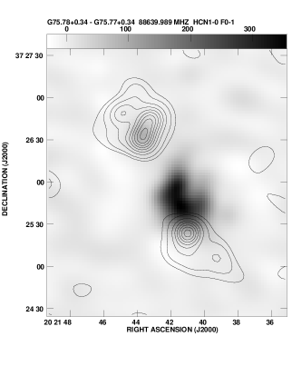
Figure 2: HCN J=1-0 F=0-1 flux contours of G75.78+0.34 and G75.77+0.34 overlaid to the the 3.5 mm continuum gray scale image

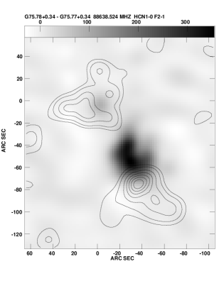
Figure 3: Same as Fig. 2 for the transition F=2-1. The position (0,0) corresponds to the location of the ultracompact H ii region G75.78+0.34.

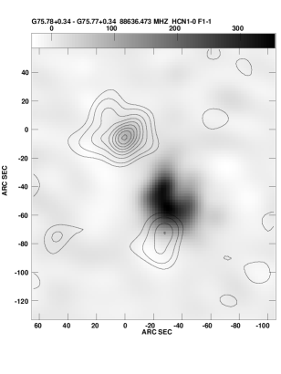
Figure 4: Same as Fig. 2 for the transition F=1-1.

A detailed inspection of Figs. 2, 3 and 4 reveals distinct morphologies for each transition at lower intensity levels. Nevertheless, the global flux distributions are similar to each other and its morphology for G75.78+0.34 can be described as asymmetric presenting two “jet-like” structures: one more extended to the east with size of $\sim 50^{\prime\prime}$ (1.3 pc) and other extending up to $\sim 40^{\prime\prime}$ (1.1 pc) north from the position of the peak intensity. A comparison of the HCN emission with the continuum image shows that it is only twice as extended as the continuum. G75.77+0.34 also presents an asymmetric morphology with a sub-structure (with size of $\sim 50^{\prime\prime}$) extended to south-east from the peak flux position and another with approximately the same size extended to south-west of it. In Table 1 we present the measured fluxes and line ratios for each H ii region.

In order to investigate the kinematics of the HCN emitting gas close to both H ii regions we have constructed velocity channel maps along each line profile with a velocity bin of 0.34 km s^-1, corresponding to our spectral sampling. The resulting velocity channel maps are shown in Figures 5, 6 and 7 for F=0–1, F=2–1 and F=1–1, respectively. The panel labeled as 8 is centred at the centroid velocity of each emission-line profile. Panels from 1 to 7 correspond to emission from blueshifted gas relative to the centroid velocity, while panels from 9 to 14 corresponds to emission from redshifted gas relative to it.

The velocity channels show that the G75.78+0.34 and G75.77+0.34 H ii regions present a complex flux distribution and kinematics, with several knots observed at distinct velocity channels and at distinct locations. At the highest blueshifts, usually G75.78+0.34 is dominated by a jet-like structure to east of the position of the peak flux, also observed in the HCN fluxes maps; as the velocities approximate to the centroid velocity the dominant structure is one elongated to north. At the highest redshifts the emission is dominated by gas located in a structure oriented east-west (clearly observed in Fig.6 panels 13 and 14). The G75.77+0.34 velocity channels are dominated a jet-like structure extended towards the south-west of the position of peak intensity in all velocities, although another emission structure extended to south-east is also present in the highest blueshifted channel maps (more clearly observed at Fig. 5).

Figure 5: Velocity channel panels along the HCN F=0-1 emission-line profile, with velocity bin of 0.34 km s${-1}$. The greyscale images show the flux distribution at each channel with intensity contours overlaid on a greyscale of the same emission. The panel 8 corresponds to the velocity of the peak of the profile and panels from 1 to 7 represents blueshifts, while panels from 9 to 14 are for redshifts relative to the peak of the profile

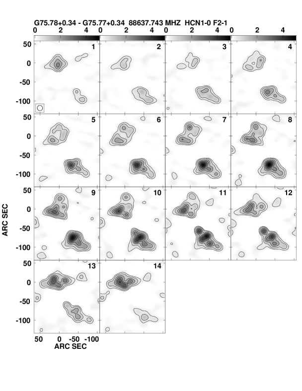
Figure 6: Same as Fig. 5 for the transition F=2-1

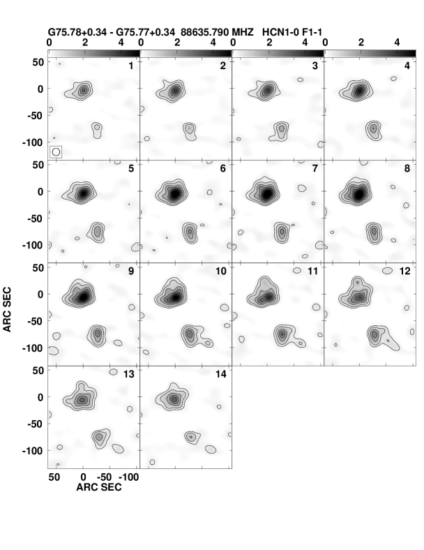
Figure 7: Same as Fig. 5 for the transition F=0-1

4 Discussion

4.1 The 3.5 mm continuum emission

Shepherd, Churchwell & Wilner (1997) used the BIMA array at configurations B and C to obtain images for the 3.5 mm continuum and molecular-line emission from H ii regions of the ON2 molecular cloud at spatial resolution of 5^′′. It is difficult to compare their continuum image with ours due to the poorer spatial resolution used in the present work. Nevertheless, we can compare the total continuum flux measured from both images. Shepherd, Churchwell & Wilner (1997) measured a total flux of 75.4 mJy for G75.78+0.34, which is about 1.5 times smaller than our measurement (119 mJy). This difference may be mostly due to the larger aperture used to integrate the flux in the present work than those used by Shepherd, Churchwell & Wilner (1997).

At millimetric wavelengths the continuum emission from H ii regions can originate from free-free emission from the ionized gas surrounding OB stars and/or by hot dust heated by nearby stars, while at higher wavelengths such as at 6 cm the radio continuum from such regions is dominated by free-free emission. Wood & Churchwell (1989) measured a flux of 40.4$\pm$0.48 mJy for G75.78+0.34 at 6 cm from VLA observations, which can be used to estimate the contribution of free-free emission to the 3.5 mm continuum under an assumption about the shape of the spectral energy distribution of G75.78+0.34. Following Shepherd, Churchwell & Wilner (1997), if we assume a nearly flat spectrum typical of optically thin free-free emission, we would predict a flux of $\sim$40 mJy for the free-free emission at 3.5 mm and thus the contribution of hot dust would be $\sim$80 mJy, about two times larger than the contribution of the free-free emission. In the case of the excess at 3.5 mm being only due to dust emission, then the peak flux should increase for lower wavelengths, which is not observed for G75.78+0.34 as discussed by Shepherd, Churchwell & Wilner (1997) based on measurements of the peak fluxes at 3.5 mm and 2.7 mm (111 GHz). Nevertheless, the discussion above is based on the assumption that G75.78+0.34 presents a flat spectrum, which may not be a good approximation of the spectral energy distribution of the region as pointed out by Franco et al. (2000a). They show that G75.78+0.34 presents a spectral index $\alpha=+1.4\pm 0.1$, suggesting that this ultracompact H ii is not optically thin, indicating a larger importance of the free-free emission to the millimetric continuum.

Garay et al. (1993) present VLA multi-frequency radio continuum images for several compact H ii regions, including G75.77+0.34. They obtained a total flux of 4.73$\pm$0.03 Jy at 20 cm, which is higher than those of the 3.5 mm emission (1.73 Jy), indicating that the millimetric continuum emission from this object is due to free-free emission in the ionized gas surrounding the O star. This conclusion is true, even we assume a negative spectral index of $\alpha=-0.1$, typical for the high frequencies (Kurtz, 2005) at optically thin regions.

A comparison between our 3.5 mm image and the 6 cm continuum image presented by Matthews & Goss (1973), for both H ii regions, shows that the two images present similar morphologies, suggesting a same origin for the continuum emission. Thus, from this comparison and from the discussion above, we conclude that the 3.5 mm continuum emission from both, G75.78+0.34 and G75.77+0.34, ultracompact H ii is dominated by free-free emission from the ionized gas surrounding the exciting stars. Nevertheless, some contribution of dust emission cannot be ruled out for G75.78+0.34.

4.2 The origin of the HCN emission

Shepherd & Churchwell (1996) presented ¹²CO(J=1–0) and ¹³CO(J=1–0) images for ten massive star formation regions obtained with the National Radio Astronomy Observatory (NRAO) Kitt Peak 12 m telescope. Their sample included both G75.77+0.34 and G75.78+0.34 objects (named by the authors as G75.78 SW and G75.78 NE, respectively). A comparison of their CO images with the HCN flux distributions (Figs. 2, 3 and 4) shows that they present similar global morphology.In the case of G75.78+0.34 we can also compare the HCN images with the CO images presented by Shepherd, Churchwell & Wilner (1997), using higher spatial resolution BIMA observations than those reached by Shepherd & Churchwell (1996). Their image present two “jet-like” structures, one to east of the ultracompact H ii region and the other to north of it, similarly to those observed in the HCN emission,although the HCN jets are less extended than the CO ones and present some knots of higher intensity levels (more clearly seen in the F=2–1 image), which are not present in the CO image. The similarity between these images suggests that the CO and HCN traces the same physical properties. Nevertheless, the smaller extension of the jets and the high emission knots in the HCN images indicate that its emission traces higher density structures than the ones traced by the CO emission, in good agreement with previous studies, which found that the J=1–0 transition from the HCN molecule is a tracer of dense cores with densities in the range $n\sim 10^{4}-10^{5}\,{\rm~{}cm^{−3}}$ (e.g. Cao et al., 1993; Afonso, Yun & Clemens, 1998).

Besides the HCN flux distribution, its emission origin is one of the most important questions in the study of molecular cores. The populations of the various molecular levels are determined by the physical parameters of the gas (temperature, density, velocity) and the intensity of each hyperfine component may be also affected by radiative transfer effects. Thus, the HCN hyperfine line ratios can be used to investigate the physical properties of the emitting gas. In Local Thermodynamic Equilibrium (LTE) the predicted theoretical values for the hyperfine line ratios for HCN(J=1–0) are $R_{02}=\frac{F=0-1}{F=2-1}=0.2$ and $R_{12}=\frac{F=1-1}{F=2-1}=0.6$ (Cernicharo et al., 1984; Harju, 1989; Afonso, Yun & Clemens, 1998). As observed in Table 1 the intensity ratios, $R_{02}$ and $R_{12}$, differ from the predicted LTE values for both H ii regions. For G75.77+0.34, $R_{02}$ is more than 3 times larger then the predicted ratio, while $R_{12}$ is 2.5 smaller. For G75.78+0.34 both ratios are larger than the theoretical values – $R_{02}$ is more than two times larger than the predicted value, while $R_{12}$ is even larger, reaching a value almost six times larger than the theoretical.

Differences between the intensity ratios observed and predicted are commonly reported in the literature and known as the hyperfine anomaly (Harju, 1989; Gonzalez-Alfonso & Cernicharo, 1993; Cao et al., 1993; Afonso, Yun & Clemens, 1998; Kim, Balasubramanyan & Burton, 2002). Two scenarios have been proposed to explain this anomaly. The thermal model developed by Guilloteau & Baudry (1981) suggests that the overlap of the J=2–1 hyperfine transitions overpopulates the state J=1, F=2, and thus the line J=1–0, F=2–1 grows relative to the other lines. With the growing temperature, the ratios $R_{02}$ and $R_{12}$ become smaller than the LTE values. This model provides a reasonable explanation for the observed ratios in hot clouds. The second scenario, proposed by Cernicharo et al. (1984), suggests that the relative intensities of HCN hyperfine transitions are formed by scattering of the radiation emitted from the cloud core to the surrounding envelope. The optically-thick lines (F=2–1 and F=1–1) are scattered more often than the optically-thin line (F=0–1), and thus the line F=0–1 is enhanced relative to the other lines.

The scattering scenario have been invoked to explain the intensity ratios observed in ultracompact H ii regions (e.g. Kim, Balasubramanyan & Burton, 2002; Harju, 1989) and could explain the emission from G75.78+0.34 and G75.77+0.34. This suggestion is supported by the distinct flux distributions observed for each hyperfine transition from both H ii regions (see Figs. 4, 3 and 2). For G75.78+0.34, the flux distribution for F=0–1 is the most concentrated, followed by F=1–1 and F=2–1, for which the scattering of the radiation emitted from the cloud core is more important. In the case of G75.77+0.34 the $R_{12}$ is smaller than the predicted for LTE, which favors the thermal model in which the intensity of F=2–1 grows relative to the other lines. Thus, numerical models and higher spatial resolution line ratio maps are necessary to properly distinguish between both scenarios for both H ii regions.

4.3 Molecular outflows

As discussed in Sec. 1, the HCN(J=1–0) and ¹²CO(J=1–0) flux distributions are similar for G75.78+0.34. From the velocity channels (Figs. 5, 6, 7) we can investigate the kinematics of the HCN emitting gas and compare it with the CO kinematics presented by Shepherd & Churchwell (1996) and Shepherd, Churchwell & Wilner (1997). These works found bipolar molecular outflows associated with the ultracompact H ii region, with the blueshifted emitting gas presenting sub-structures elongated to north and to east from the peak flux position and the redshifted gas being more elongated to south-west of it. A detailed analysis of the HCN velocity channels reveals that the blueshifted HCN emission is dominated by the two “jet-like” structures described above.The peak of redshifted HCN emission is a bit displaced to south relative to the peak position of the blueshifted emission and the highest velocity channels present an additional structure extended to south-west. These kinematic components are similar to those observed in ¹²CO(J=1–0) indicating that at least part of the HCN emitting gas follow the bipolar molecular outflows observed in CO.

In the case of G75.77+0.34 there are no velocity channel maps with similar resolution to ours for the CO emission in the literature and thus a comparison between the HCN and CO kinematics is not possible here. The flux distribution of all channel maps are similar, with exception of the highest velocity channels, which show three knots oriented to south-west of the position of the peak emission, indicating that dense molecular outflows are less important for this object than for the case of G75.78+0.34.

5 Conclusions

We analyzed 3.5 mm continuum and HCN(J=1–0) line emission from the H ii regions G75.78+0.34 and G75.77+0.34 from interferometric observations obtained with the BIMA array in D configuration. We present for the first time images for the HCN(J=1–0) for both H ii regions. The main results of this work are:

• The the 3.5 mm continuum emission is consistent with the free-free emission from the ionized gas from the H ii regions. However, the contribution of emission from hot dust cannot be totally discarded for G75.78+0.34.

• The flux distributions for the HCN(J=1–0) hyperfine lines present similar structures than those observed in ¹²CO(J=1–0) images, suggesting both gases traces the same physical conditions. Some knots of high intensity are present only in the HCN images suggesting the presence of high density regions not observed in CO.

• The analysis of the HCN(J=1–0) hyperfine intensity ratios reveals that they are different than those predicted theoretically for LTE, probably due to scattering of radiation processes.

• The kinematical analysis reveal that the HCN emitting gas follows the bipolar molecular outflows observed in CO for G75.78+0.34, while for G75.77+0.34 the outflows seems to be less important.

References

- Afonso, Yun & Clemens (1998) Afonso, J. M., Yun, J. L., & Clemens, D. P., 1998, AJ, 115, 1111
- Cao et al. (1993) Cao, Y. X.;, Zeng, Q., Deguchi, S., Kameya, O. & Kaifu, N., 1993, AJ, 105, 1027.
- Carral et al. (1997) Carral, P., Kurtz, S. E., Rodríguez, L. F., De Pree, C., & Hofner, P., 1997, ApJ, 486, L103.
- Cernicharo et al. (1984) Cernicharo, J., Castets, A., Duvert, G., Guilloteau, S., 1984, A&A, 139, L13
- Franco et al. (2000a) Franco, J., Kurtz, S., Hofner, P., Testi, L., García-Segura, G., & Martos, M., 2000, ApJ, 542, L143.
- Franco et al. (2000b) Franco, J., Kurtz, S., García-Segura, G., & Hofner, P., 2000, APSS, 272, 179.
- Garay et al. (1993) Garay, G., Rodríguez, L. F., Moran, J. M., & Churchwell, E., 1993, ApJ, 418, 368.
- Gonzalez-Alfonso & Cernicharo (1993) Gonzalez-Alfonso, E. & Cernicharo, J., 1993, A&A, 279, 506.
- Guilloteau & Baudry (1981) Guilloteau, S., & Baudry, A., 1981, A&A, 97, 213.
- Habing & Israel (1979) Habing, H. J., Israel, F. P., 1979, ARAA, 17, 345.
- Hofner & Churchwell (1996) Hofner, P., & Churchwell, E., 1996, A&AS, 120, 283.
- Harju (1989) Harju, J., 1989, A&A, 219, 293.
- Kim, Balasubramanyan & Burton (2002) Kim, H., Balasubramanyan, R., & Burton, M. G., 2002, PASA, 19, 505.
- Kurtz, Churchwell & Wood (1994) Kurtz, S., Churchwell, E., & Wood, D. O. S., 1994, ApJS, 91, 959.
- Kurtz (2005) Kurtz, S., 2005, Proceedings IAU Symposium 227, Massive Star Birth: A Crossroads of Astrophysics, R. Cesaroni, M. Felli, E., Churchwell & C. M. Walmsley, eds. pg. 111.
- Matthews & Goss (1973) Mattews, H. E., & Goss, W. M., 1973, A&A, 29, 309.
- Matthews, Andersson & Mcdonald (1986) Matthews, N., Andersson, M., & Mcdonald, G. H., 1986, A&A, 155, 99
- Qin et al. (2008) Qin, S., Wang, J., Zhao, G., Miller, M., & Zhao, J., 2008, A&A, 484, 361.
- Roman-Lopes et al. (2009) Roman-Lopes, A., Abraham, Z., Ortiz, R., & Rodríguez-Ardila, A., 2009, MNRAS, 394, 467.