Dynamical Casimir effect with Robin boundary conditions
in a three dimensional open cavity

Abstract

We consider a massless scalar field in 1+1 dimensions inside a cavity composed by a fixed plate, which imposes on the field a Robin BC, and an oscillating one, which imposes on the field a Dirichlet BC. Assuming that the plate moves for a finite time interval, and considering parametric resonance, we compute the total number of created particles inside the cavity. We generalize our results to the case of two parallel plates in 3+1 dimensions.

I Introduction

The dynamical Casimir effect (DCE) consists of two related phenomena: real particle creation due to moving boundaries and radiation reaction forces on moving boundaries. This effect already manifests itself for a unique moving plate and, for a non-relativistic motion, the frequencies of the created particles (photons in the case of the quantized electromagnetic field) are smaller or equal than the mechanical frequency of the moving plate. Since Moore’s pioneering paperMoore70 , the DCE has been studied in many different situations by many authors (for a review on this subject see DodonovReview and the special issue SpecialIssue ). Particularly, many distinct boundary conditions (BC) have been considered, from the idealized Dirichlet and Neumann ones to more realistic ones. However, the so called Robin boundary conditions (RBC), which interpolate continuously Dirichlet and Neumann ones, have rarely been used explicitly in the context of the DCE (though they have been considered by many authors in the context of the static Casimir effect, see for instance Romeo-Saharian-2002 ). As far as we know, RBC appeared in the DCE only for the situation of one moving plate in 1+1 dimensions Bruno-1 ; Bruno-2 . Our purpose here is to consider RBC in one-dimensional cavities with one oscillating wall and in three-dimensional (open) cavities formed by two parallel plates with one of them oscillating in time. For a scalar field $\phi$ in 3+1 dimensions, RBC are defined by $\phi|_{bound.}=\beta\frac{\partial\phi}{\partial n}|_{bound.}$ where $\beta$ is a constant parameter with dimension of length. They interpolate continuously Dirichlet ($\beta\to 0$) and Neumann ($\beta\to\infty$) BC. They appear in different areas of physics: from Mechanics, Electromagnetism and Quantum Mechanics to Quantum Field Theory, among others. These BC were used as a phenomenological model for penetrable surfaces Mostepanenko-Trunov-1985 . In fact, for $\omega\ll\omega_{P}$, parameter $\beta$ plays the role of the plasma wavelength. In Classical Mechanics, RBC may appear in a vibrating string coupled to a harmonic oscillator at one of its edges Chen-Zhou-1992 ; Bruno-1 . In the context of the static Casimir effect, RBC lead to eigenfrequencies for the cavity modes that are roots of a transcendental equation.

In the context of the Dynamical Casimir effect, Mintz et al Bruno-1 considered a massless scalar field $\phi$ in $1+1$ dimensions under the influence of one moving boundary in a prescribed and non-relativistic motion with small amplitudes, namely, $|\delta\dot{q}(t)|<<c$ and $|\delta q(t)|<<c/\omega_{0},$ where $\delta q(t)$ is the position of the moving boundary at instant $t$ and $\omega_{0}$ is the dominant mechanical frequency. Using the perturbative approach of Ford and Vilenkin Ford-Vilenkin-1982 , the solution of the wave equation, $\partial^{2}\phi(t,x)=0$, submitted to a RBC, leads to a susceptibility with both real and imaginary parts, so that, $\delta{\mathcal{F}}(\omega)={\chi(\omega)}\delta Q(\omega)$, with $\chi(\omega)={\mathcal{R}}e\chi(\omega)+i{\mathcal{I}}m\chi(\omega).$ Recall that, for the same situation, the use of a Dirichlet (or Neumann) BC would lead to a purely imaginary susceptibility $\chi\!_{{\,}_{D}}(\omega)=\omega^{3}/6\pi$, (${c=\hbar=1}$). For a typical oscillatory motion, given by $\delta q(t)=\delta q_{0}\,e^{-|t|/T}\!\!\cos(\omega_{0}t),$ with $\omega_{0}T\gg 1,$ Mintz et al Bruno-1 showed that the dissipative force on the moving boundary can be enormously suppressed for $\beta\omega_{0}\approx 2$. In a subsequent paper Bruno-2 , these authors analyzed the particle creation phenomenon for the same situation and found that, for the above mentioned relation between $\beta$ and $\omega_{0}$, there is also an enormous suppression of particle creation.

II One-dimensional cavities with Robin BC

For simplicity, we consider a one-dimensional cavity composed by a fixed plate at $x=0$, which imposes on the massless scalar field a RBC, and a moving plate whose position at instant $t$ is given by $q(t)$, which imposes on the field a Dirichlet BC. Then, we must solve the wave equation with $\hat{\phi}$ submitted to $\left(\hat{\phi}(x,t)-\gamma\frac{\partial}{\partial x}\hat{\phi}(x,t)\right)\big{|}_{x=0}\!=\!0\;\mbox{and}\;\hat{\phi}(x,t)\big{|}_{x=q(t)}\!=\!0.$ The scalar field satisfies the usual field commutation relations, namely, $\left[\hat{\phi}(x;t),\hat{\pi}(x^{\prime};t)\right]=i\delta(x^{\prime}-x),$ and $\left[\hat{\phi}(x;t),\hat{\phi}(x^{\prime};t)\right]=\left[\hat{\pi}(x;t),\hat{\pi}(x^{\prime};t)\right]=0,$ Our anstaz for the field operators $\hat{\phi}$ and $\hat{\pi}=\dot{\hat{\phi}}$ in terms of the instantaneous basis introduced by LawLaw-1994 , in 1994, is

$$\hat{\phi}(x;t) = \sum_{n}\frac{1}{\sqrt{2k_{n}(t)}}\;u_{n}(x;t)\Bigl{\{}\hat{\textsl{a}}_{n}(t)+\hat{\textsl{a}}_{n}^{{\dagger}}(t)\Bigr{\}}$$ (1)

$$\hat{\pi}(x;t) = -i\sum_{n}\sqrt{\frac{k_{n}(t)}{2}}\;u_{n}(x;t)\Bigl{\{}\hat{\textsl{a}}_{n}(t)-\hat{\textsl{a}}_{n}^{{\dagger}}(t)\Bigr{\}},$$ (2)

where the modes $\{u_{n}(x,t)\}$ of the instantaneous basis must satisfy Helmholtz equation, $\left(\frac{\partial^{2}}{\partial x^{2}}+k_{n}^{2}(t)\right)u_{n}(x;t)=0,$ the boundary conditions $\left(u_{n}(x,t)-\gamma\frac{\partial\ }{\partial x}u_{n}(x,t)\right)|_{x=0}=0$ and $u_{n}(x,t)|_{x=q(t)}=0\,,$ and the orthonormality condition $\int_{0}^{q(t)}\!\!\mbox{d}xu_{n}(x;t)u_{m}(x;t)\!=\!\delta_{nm}$. With these properties, it follows that $\left[\textsl{a}_{n}(t),\textsl{a}_{m}^{{\dagger}}(t)\right]=\delta_{nm}$ and $\left[\textsl{a}_{n}^{{\dagger}}(t),\textsl{a}_{m}^{{\dagger}}(t)\right]=\left[\textsl{a}_{n}(t),\textsl{a}_{m}(t)\right]=0.$ The instantaneous basis can be explicitly obtained, with modes $u_{n}(x,t)$ given by

$$u_{n}(x;t)=\frac{A_{n}(t)}{\sqrt{2q(t)}}\sin\Bigl{[}k_{n}(t)(x-q(t))\Bigr{]},$$ (3)

where $A_{n}(t)=2\left[1+\frac{\gamma/q(t)}{1+\gamma^{2}k_{n}^{2}(t)}\right]^{-1/2}$ and $\{k_{n}(t)\}$ are the roots of the following transcendental equation $\sin[q(t)k_{n}(t)]+\gamma k_{n}(t)\cos\bigl{[}q(t)k_{n}(t)\bigr{]}=0.$

Time evolution equations for ${\hat{a}}_{n}(t)$ and ${\hat{a}}^{\dagger}_{n}(t)$ can be found,

$$\dot{\hat{\textsl{a}}}_{n}(t)=-ik_{n}(t)\hat{\textsl{a}}_{n}(t)+\sum_{j}\Xi_{jn}(t)\hat{\textsl{a}}_{j}(t)+\sum_{j}\Lambda_{jn}(t)\hat{\textsl{a}}_{j}^{{\dagger}}(t)\,,$$ (4)

where

$$\Xi_{mn}(t) := -\frac{1}{2}G_{mn}(t)\left(\sqrt{\frac{k_{n}(t)}{k_{m}(t)}}+\sqrt{\frac{k_{m}(t)}{k_{n}(t)}}\right);$$ (5)

$$\Lambda_{mn}(t) := \frac{\dot{k}_{n}(t)}{2k_{n}(t)}\delta_{mn}-\frac{1}{2}G_{mn}(t)\left(\sqrt{\frac{k_{n}(t)}{k_{m}(t)}}-\sqrt{\frac{k_{m}(t)}{k_{n}(t)}}\right)\,,$$ (6)

with $G_{nm}(t):=\int_{0}^{q(t)}\mbox{d}x\ \dot{u}_{n}(x;t)u_{m}(x;t)$ (an analogous equation holds for ${\hat{a}}^{\dagger}_{n}(t)$)). Relating $\hat{\textsl{a}}_{n}$ and $\hat{\textsl{a}}_{n}^{{\dagger}}$ for different times, we write

$$\hat{\textsl{a}}_{n}(t)=\sum_{m}\alpha_{nm}(t)\hat{\textsl{a}}_{m}(t_{0})+\sum_{m}\beta_{nm}(t)\hat{\textsl{a}}_{m}^{{\dagger}}(t_{0})\,,$$ (7)

where the Bogoliubov coefficients must satisfy $\alpha_{nm}(t_{0})=\delta_{nm}$ and $\beta_{nm}(t_{0})=0$. The time evolution of these coefficients can be established,

$$\dot{\alpha}_{nm}(t)\! = \!-ik_{n}(t)\alpha_{nm}(t)+\sum_{j}\Xi_{jn}(t)\alpha_{jm}(t)+\sum_{j}\Lambda_{jn}(t)\beta_{jm}^{\ast}(t);$$ (8)

$$\dot{\beta}_{nm}(t)\! = \!-ik_{n}(t)\beta_{nm}(t)+\sum_{j}\Xi_{jn}(t)\beta_{jm}(t)+\sum_{j}\Lambda_{jn}(t)\alpha_{jm}^{\ast}(t).$$ (9)

Previous equations may be simplified with the aid of definitions:

$$\alpha_{nm}(t) =: \mbox{e}^{-iK_{n}(t)}\tilde{\alpha}_{nm}(t)\,;\;\;\;\;\beta_{nm}(t)=:\mbox{e}^{-iK_{n}(t)}\tilde{\beta}_{nm}(t)\,;\;\;\;\;$$ (10)

$$K_{n}(t) := \int_{t_{0}}^{t}\mbox{d}t^{\prime}\ k_{n}(t^{\prime});$$ (11)

$$\Xi_{mn}(t) =: \tilde{\Xi}_{mn}(t)\mbox{e}^{i\left[K_{m}(t)-K_{n}(t)\right]}\,;\;\;\Lambda_{mn}(t)=:\tilde{\Lambda}_{mn}(t)\mbox{e}^{-i\left[K_{m}(t)+K_{n}(t)\right]}\;,$$

Consequently, the time evolution for coefficients ${\tilde{\alpha}}_{nm}$ and ${\tilde{\beta}}_{nm}$ are

$$\dot{\tilde{\alpha}}_{nm}(t) = \sum_{j}\tilde{\Xi}_{jn}(t)\tilde{\alpha}_{jm}(t)+\sum_{j}\tilde{\Lambda}_{jn}(t)\tilde{\beta}_{jm}^{\ast}(t);$$ (12)

$$\dot{\tilde{\beta}}_{nm}(t) = \sum_{j}\tilde{\Xi}_{jn}(t)\tilde{\beta}_{jm}(t)+\sum_{j}\tilde{\Lambda}_{jn}(t)\tilde{\alpha}_{jm}^{\ast}(t)\;.$$ (13)

Up to this point, our calculations are exact. However, from now on, we shall consider only oscillating motions with small amplitudes, so we write $q(t)=q_{0}[1+{\epsilon}\xi(t)]$, with ${\epsilon\ll 1}$ and $\xi(t)$ given, for a typical motion, by

$$\xi(t)=\begin{cases}\sin(\omega_{0}t)&0<t<t_{f}\\ 0&t\leq 0\text{ or }t\geq t_{f}\;.\end{cases}$$

Expansions in powers of $\epsilon$ (recall that all quantities get an implicit $\epsilon$-dependence through $q(t)$) lead to

$$\tilde{\alpha}_{nm}^{(\ell)}(t)\! = \!\sum_{\ell^{\prime}=1}^{\ell}\sum_{j}\int_{t_{0}}^{t}\mbox{d}\tau\left[\tilde{\Xi}_{jn}^{(\ell^{\prime})}(\tau)\tilde{\alpha}_{jm}^{(\ell-\ell^{\prime})}(\tau)+\tilde{\Lambda}_{jn}^{(\ell^{\prime})}(\tau)\tilde{\beta}_{jm}^{\ast(\ell-\ell^{\prime})}(\tau)\right];$$ (14)

$$\tilde{\beta}_{nm}^{(\ell)}(t)\! = \!\sum_{\ell^{\prime}=1}^{\ell}\sum_{j}\int_{t_{0}}^{t}\mbox{d}\tau\left[\tilde{\Xi}_{jn}^{(\ell^{\prime})}(\tau)\tilde{\beta}_{jm}^{(\ell-\ell^{\prime})}(\tau)+\tilde{\Lambda}_{jn}^{(\ell^{\prime})}(\tau)\tilde{\alpha}_{jm}^{\ast(\ell-\ell^{\prime})}(\tau)\right]\,.$$ (15)

where the superscritps mean the order of the derivative respect to $\epsilon$ of the quantity in question and conditons $\tilde{\alpha}_{nm}^{(0)}(t)=\delta_{nm}$ and $\tilde{\beta}_{nm}^{(0)}(t)=0$ are satisfied. The number of particles created inside the cavity, with energy $\omega_{n}=k_{n}$, after the motion is finished is given by

$$\mathcal{N}_{n}(t_{f})=\left\langle 0\right|\hat{\textsl{a}}_{n}^{{\dagger}}\left(t_{f}\right)\hat{\textsl{a}}_{n}\left(t_{f}\right)\left|0\right\rangle=\sum_{j}\left|\sum_{\ell}\epsilon^{\ell}{\beta}^{(\ell)}_{nj}(t_{f})\right|^{2}.$$ (16)

The first correction to $\mathcal{N}_{n}(t_{f})$ occurs at order $\epsilon^{2}$,

$$\mathcal{N}_{n}(t_{f})=\epsilon^{2}\sum_{m}\left|\beta_{nm}^{(1)}(t_{f})\right|^{2}=\epsilon^{2}\sum_{m}\left|\tilde{\beta}_{nm}^{(1)}(t_{f})\right|^{2}\,,$$ (17)

For the motion in consideration, we have

$$\mathcal{N}_{n}(t_{f})=\sum_{m}\left|\mathcal{C}_{nm}(\gamma)f_{nm}(\omega_{0},t_{f})\right|^{2}\left(\epsilon\omega_{0}t_{f}\right)^{2}.$$ (18)

where

$$f_{nm}(\omega_{0};t) {:=} \frac{e^{i(\omega_{0}+\kappa_{nm})t}\;-\;1}{(\omega_{0}+\kappa_{nm})t\;\;}\;-\;\frac{e^{-i(\omega_{0}-\kappa_{nm})t}\;-\;1}{(\omega_{0}-\kappa_{nm})t\;\;}$$ (19)

$$C_{nm}(\gamma) = \frac{1}{8}A_{n}(0)A_{m}(0)\frac{\sqrt{k_{n}(0)k_{m}(0)}}{k_{n}(0)+k_{m}(0)}\;,$$ (20)

$$\kappa_{nm} = k_{n}(0)+k_{m}(0)\,.$$

At this order, the total number of particles created inside the cavity is given by $\mathcal{N}=\sum\!\!\!\!\!\!\!\!\!_{{\,}\atop{{\,}_{n,m}}}\left|\mathcal{C}_{nm}(\gamma)f_{nm}(\omega_{0},t_{f})\right|^{2}\left(\epsilon\omega_{0}t_{f}\right)^{2}$ while the total energy of the created particles is given by $\mathcal{E}=\sum\!\!\!\!\!\!\!\!\!_{{\,}\atop{{\,}_{n,m}}}k_{n}\left|\mathcal{C}_{nm}(\gamma)f_{nm}(\omega_{0},t_{f})\right|^{2}\left(\epsilon\omega_{0}t_{f}\right)^{2}.$ The behavior of $|f_{nm}(\omega_{0};t_{f})|^{2}$ is shown in Figure 1. For $\omega_{0}t_{f}\gg 1$, it has a peak around $\omega_{0}=\kappa_{mn}$ whose width $\delta$ is proportional to $1/(\kappa_{nm}t_{f})$ (a simple estimative gives $\delta\approx 5.6/(\kappa_{nm}t_{f})$). Hence, in a first approximation, $|f_{nm}(\omega_{0};t_{f})|^{2}$ behaves like a delta function, showing that whenever the oscillation frequency $\omega_{0}$ equals the sum of two energy levels of the corresponding static cavity we have the best conditions for particle creation.

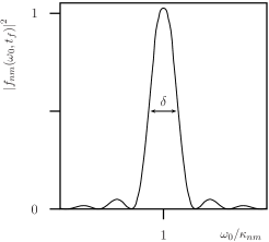
Figure 1: $|f_{nm}(\omega_{0};t_{f})|^{2}$ as a function of $\omega_{0}/\kappa_{nm}$ for $\omega_{0}t_{f}\gg 1$.

The fact that $\kappa_{mn}$ is given by a sum of 2 terms means that particles are created in pairs. The set of values of $\kappa_{mn}$ are called the resonances of the problem. Note that, for each value of the Robin parameter, $\gamma$, we have a different set of resonances. Figure 2 shows how the resonances vary with $\gamma$. Since $\gamma$ varies from $0$ (Dirichlet BC) to $\infty$ (Neumann BC), it is convenient to make the plot against $log_{10}(\gamma/q_{0})$, instead of $\gamma$.

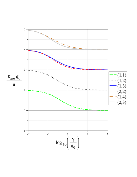
Figure 2: Resonances (in units of $\pi/q_{0}$) as functions of $\log_{10}(\gamma/q_{0})$.

For a given value of $\gamma$, the resonances are obtained by tracing a vertical line and looking at the intersections in Figure 2. The values obtained this way for $\log_{10}(\gamma/q_{0})=-2$ (extreme left on the graph) are, approximately, the resonances for Dirichlet-Dirichlet BC since, for this case, $\gamma\ll q_{0}$. By the same token, the values obtained this way for $\log_{10}(\gamma/q_{0})=2$ (extreme right on the graph) are, approximately, the resonances for Neumann-Dirichlet BC since, for this case, $\gamma\gg q_{0}$. Adjacent resonances are equally spaced only for D-D and N-D cases. For these cases we have degeneracies, which are broken in the Robin-Dirichlet case. For instance, for this last case, $\kappa_{13}=k_{1}+k_{3}\neq k_{2}+k_{2}=\kappa_{22}$, as can be seen in Figure 2 near $\log_{10}(\gamma/q_{0})=0$. Note, also, the monotonic behavior of the curves with $\gamma/q_{0}$.

Figure 3 shows the number of created particles with energy $k_{1}$ for different resonant values of the mechanical frequency as a function of $\log_{10}(\gamma/q_{0})$ (since particles are created in pairs, there are many ways of creating particles with energy $k_{1}$, namely, $\omega_{0}=\kappa_{11}$, $\omega_{0}=\kappa_{12}$, etc.). For the resonance $\omega_{0}=\kappa_{1m}$, we have $N_{1m}=\mathcal{C}^{2}_{1m}(\gamma)\left(\epsilon\kappa_{1m}t_{f}\right)^{2}$.

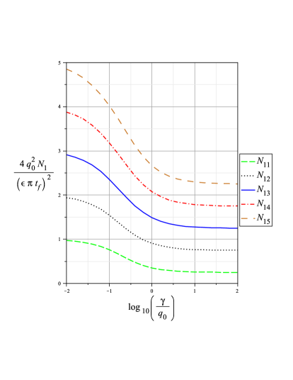
Figure 3: Number of created particles with energy $k_{1}(0)$ (in units of $\left(\frac{\epsilon\pi t_{f}}{2q_{0}}\right)^{2}$ for the first five resonant values of $\omega_{0}$p as a function of $\log_{10}(\gamma/q_{0})$.

It is worth saying a few words about how the curves in Figure 3 are traced. For each value of $\gamma$, we compute numerically the set of corresponding resonances. Then, we compute $N_{11}$, $N_{12}$, $N_{13}$, …, for that value of $\gamma$. We, then, take another value of $\gamma$ and compute the new values of the resonances. Taking $\omega_{0}$ equal to the new values of resonances we compute again $N_{11}$, $N_{12}$, $N_{13}$, and so on. Hence, distinct points of a given curve, for instance $N_{1}$, are computed with distinct values of $\omega_{0}$, but with $\omega_{0}$ always equal to the first resonance ($\kappa_{11}$, which depends on $\gamma$). Note, also, the monotonic behavior of curves in Figure 3.

Let us check some particular cases. For $\omega_{0}=\frac{2\pi}{q_{0}}$ and $\gamma=0$, which corresponds to the D-D case with $\omega_{0}=2k_{1}$ (parametric resonance with the lowest level of the static cavity), we have $\mathcal{N}_{1}\simeq\left(\frac{\epsilon\pi t_{f}}{2q_{0}}\right)^{2}$ and $\mathcal{E}_{1}\simeq\frac{\pi}{q_{0}}\left(\frac{\epsilon\pi t_{f}}{2q_{0}}\right)^{2}$ in agreement with Dodonov and Klimov Dodonov-Klimov-1996 . For $\omega=\frac{\pi}{q_{0}}$ and $\gamma\rightarrow\infty$, which corresponds to the N-D case with $\omega_{0}=2k_{1}$ (parametric resonance with the lowest level of the static cavity, which is $\frac{1}{2}$ the value for the D-D case), we have $\mathcal{N}_{1}\simeq\left(\frac{\epsilon\pi t_{f}}{4q_{0}}\right)^{2}$ and $\mathcal{E}_{1}\simeq\frac{\pi}{2q_{0}}\left(\frac{\epsilon\pi t_{f}}{4q_{0}}\right)^{2},$ in agreement with Alves et al AlvesEtAl-2006 .

III Parallel plates in 3+1 dimensions with Robin BC

Here, we shall generalize some of the previous results to 3+1 dimensions. We, then, consider a fixed plate at $z=0$, which imposes on a massless scalar field a RBC and a moving plate, parallel to the first one, which imposes on the field a DBC. Let $q(t)$ be the position of the moving plate at instant $t$. Operators $\hat{\phi}\left(\mathbf{x};t\right)$ and $\hat{\pi}\left(\mathbf{x};t\right)$ are given, in terms of instantaneous basis, by

$$\hat{\phi}\left(\mathbf{x};t\right)\! = \!\sum_{n=1}^{\infty}\int\frac{\mbox{d}^{2}\mathbf{k}_{\|}}{\sqrt{2\omega_{n}\left(k_{\|},t\right)}}~{}u_{n}\left(x;t\right)\left[\frac{\mbox{e}^{i\mathbf{k}_{\|}\cdot\mathbf{x}}}{2\pi}\hat{a}_{n}\left(\mathbf{k}_{\|},t\right)+\mbox{h.c.}\right],$$ (21)

$$\hat{\pi}\left(\mathbf{x};t\right)\!\! = \!\!-i\sum_{n=1}^{\infty}\!\!\int\!\!\mbox{d}^{2}\mathbf{k}_{\|}~{}\!\!\sqrt{\frac{\omega_{n}\left(k_{\|},t\right)}{2}}~{}\!\!u_{n}\left(x;t\right)\!\!\left[\frac{\mbox{e}^{i\mathbf{k}_{\|}\cdot\mathbf{x}}}{2\pi}\hat{a}_{n}\left(\mathbf{k}_{\|},t\right)-\mbox{h.c.}\!\right]$$ (22)

where $\omega_{n}^{2}\left(k_{\|},t\right)\!=\!k_{\|}^{2}+k_{n}^{2}(t)$ and $u_{n}\left(x,t\right)\!=\!\!\sqrt{\frac{2}{q(t)}}{A_{n}(t)}\sin\bigl{[}{k_{n}(t)}\left(x-q(t)\right)\bigr{]},$ with $A_{n}(t)$ and $k_{n}(t)$ defined as in the 1+1 case. We shall consider the same motion as in the 1+1 case. The Bogoliubov coefficients are now defined by

$$\hat{a}_{n}\left(\mathbf{k}_{\|},t\right)=\sum_{m=0}^{\infty}\left[\alpha_{nm}\left(k_{\|},t\right)\hat{a}_{m}\left(\mathbf{k}_{\|},0\right)+\beta_{nm}\left(k_{\|},t\right)\hat{a}_{m}^{{\dagger}}\left(-\mathbf{k}_{\|},0\right)\right].$$ (23)

A perturbative solution, up to first order in $\epsilon$, leads to

$$\beta_{nm}\left(k_{\|},t\right)\mbox{e}^{i\omega_{n}\left(k_{\|}\right)t}=-\epsilon\,C_{nm}\left(k_{\|}\right)f_{nm}\left(k_{\|},t\right),$$ (24)

where we defined

$$C_{nm}\left(k_{\|}\right) = \frac{A_{n}(0)A_{m}(0)}{\sqrt{\omega_{m}\left(k_{\|}\right)\omega_{n}\left(k_{\|}\right)}}\frac{k_{n}(0)k_{m}(0)}{\omega_{n}\left(k_{\|}\right)+\omega_{m}\left(k_{\|}\right)},$$ (25)

$$f_{nm}\left(k_{\|},t\right) = \int_{0}^{t}\mbox{d}t^{\prime}\dot{\xi}(t^{\prime})\mbox{e}^{i\left[\omega_{m}\left(k_{\|}\right)+\omega_{n}\left(k_{\|}\right)\right]t^{\prime}}$$ (26)

with $\omega_{n}^{2}\left(k_{\|}\right)=\omega_{n}^{2}\left(k_{\|},0\right)$. The number of created particles in a given mode with $k_{z}=k_{n}$ and with a parallel moment between $\mathbf{k}_{\|}$ and $\mathbf{k}_{\|}+$d${}^{2}\mathbf{k}_{\|}$ is

$$\mathcal{N}_{n}\left(\mathbf{k}_{\|},t_{f}\right)\mbox{d}^{2}\mathbf{k}_{\|}=\epsilon^{2}\frac{L^{2}}{\left(2\pi\right)^{2}}\sum_{m=1}^{\infty}\left|C_{nm}\left(k_{\|}\right)f_{nm}\left(k_{\|},t_{f}\right)\right|^{2}\mbox{d}^{2}\mathbf{k}_{\|}.$$ (27)

The total number of created particles inside the cavity takes the form

$$\mathcal{N}\left(t_{f}\right)=\epsilon^{2}\frac{L^{2}}{2\pi}\sum_{n,m=1}^{\infty}\int_{0}^{\infty}\mbox{d}k_{\|}~{}k_{\|}\left|C_{nm}\left(k_{\|}\right)f_{nm}\left(k_{\|},t_{f}\right)\right|^{2},$$ (28)

and the total energy is given by

$$\mathcal{E}\left(t_{f}\right)=\epsilon^{2}\frac{L^{2}}{2\pi}\sum_{n,m=1}^{\infty}\int_{0}^{\infty}\mbox{d}k_{\|}~{}k_{\|}\omega_{m}\left(k_{\|}\right)\left|C_{nm}\left(k_{\|}\right)f_{nm}\left(k_{\|},t_{f}\right)\right|^{2}.$$ (29)

For the harmonic motion considered before, with $\omega t_{f}\gg 1$), we get

$$\left|f_{nm}\left(k_{\|},t_{f}\right)\right|^{2} = \frac{\pi\omega^{2}t_{f}}{4k_{\|}}\left(\frac{\omega_{n}\left(k_{\|}\right)\omega_{m}\left(k_{\|}\right)}{\omega_{n}\left(k_{\|}\right)+\omega_{m}\left(k_{\|}\right)}\right)\delta\left(k_{nm}(\omega)-k_{\|}\right),$$ (30)

where $\sqrt{k_{nm}^{2}(\omega)+k_{n}^{2}}+\sqrt{k_{nm}^{2}(\omega)+k_{m}^{2}}-\omega=0.$ Using last result for $\left|f_{nm}\left(k_{\|},t_{f}\right)\right|^{2}$, we obtain

$$\mathcal{N}\left(t_{f}\right)=\epsilon^{2}\frac{L^{2}t_{f}}{8\omega}\sum_{n,m=1}^{\infty}\left(A_{n}A_{m}k_{n}k_{m}\right)^{2}\Theta\left(\omega-k_{n}-k_{m}\right)$$ (31)

and $\mathcal{E}\left(t_{f}\right)=\mathcal{N}\left(t_{f}\right)\omega/2$. Figure 4 shows the behavior of the total number of created particles inside the plates in terms of the frequency $\omega$ of the moving plate. We plot $\mathcal{N}\left(t_{f}\right)$ divided by $\epsilon^{2}\omega^{3}L^{2}t_{f}$ in terms of $\omega a_{0}/\pi$.

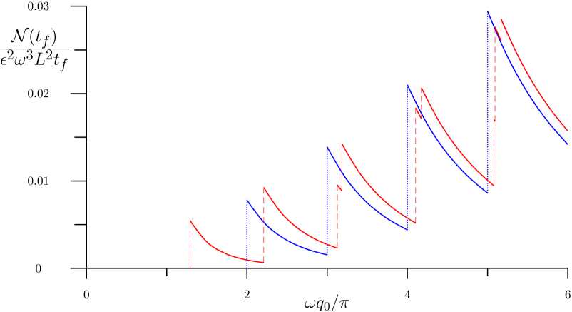
Figure 4: Total number of created particles for an open three-dimensional cavity formed by two parallel plates as a function of the frequency of the moving plate.

Solid lines connected by dotted lines correspond to the DD case, while solid lines connected by dashed lines, to a RD case. The discontinuities occur at the resonant values ($\omega=k_{n}+k_{m}$). The main difference between DD and RD cases consists in the fact that the resonances for the former are equally spaced, while for the latter they are not equally spaced, as can be seen from Figure 4. Note the presence of small solid lines for the RD case, a direct consequence of the degeneracy breaking that happens when we use RBC, as discussed previously. It is worth noting the similarity of the graph for the D-D case with that for the electromagnetic field inside two parallel and perfectly conducting plates discussed by Mundarain and Maia NetoMundarain-PAMN-1998 .

IV Final comments

In this work we considered RBC in one-dimensional cavities and in a three-dimensional open cavity formed by two parallel plates. Using the instantaneous basis method Law-1994 we computed the number of created particles when the frequency of the oscillating plate was at resonance. As we showed, for one-dimensional cavities, there are more resonances for the RD case than for the DD or ND cases, due to the degeneracy breaking discussed in the text. For the same reason, there are more discontinuities in Figure 4 when a RBC is involved than for the case where both plates impose a DBC on the field. An important difference between the 1+1 and 3+1 cases treated here is that in the former the total number of created particles, $\mathcal{N}\left(t_{f}\right)$, is proportional to $t_{f}^{2}$, while in the latter, $\mathcal{N}\left(t_{f}\right)$ is proportional to $t_{f}$, as shown in equations (18) and (31). This occurs because in the 1+1 case we have a closed cavity, while the system formed by two parallel plates correspond, in fact, to an open cavity.

The possibility of suppression of the DCE Bruno-1 ; Bruno-2 was not investigated, since we considered here always resonant cavities. It would be interesting to study a massless scalar field in 3+1 dimensions submitted to a RBC at one moving plate and check if suppression of the DCE still occurs. We think that RBC, as well as more realistic BC, should be more investigated in the DCE, whose experimental verification seems imminent BraggioEtAl-2005 (see also the recent proposal of experiment Squid-2009 ). In this work we were concerned only with the regions inside the cavities, but an analysis involving also the outside regions, including a discussion of the dissipative force on the moving plate and the energy balance, can be made and will appear elsewhere.

Acknowledgments: C.F. would like to thank CNPq and Faperj for a partial financial support.

References

• (1) GT Moore, J. Math. Phys. 11 (1970) 2679
• (2) VV Dodonov, Modern Nonlinear Optics, Advances in Chem. Phys. Series 119, 309, ed. MW Evans (Wiley, New York, 2001)
• (3) Special Issue on the Non-stationary Casimir effect and quantum systems with moving boundaries, J. Opt. B: Quantum Semiclass. Opt. 7 S3 (2005)
• (4) A Romeo and AA Saharian, J. Phys. A35 (2002) 1297
• (5) B Mintz, C Farina, PA Maia Neto and R Rodrigues, J. Phys. A39 (2006) 6559
• (6) B Mintz, C Farina, PA Maia Neto and R Rodrigues, J. Phys. A39 (2006) 11325
• (7) VM Mostepanenko and NN Trunov, Sov. J. Nucl. Phys. 45 (1985) 818
• (8) G Chen and J Zhou, Vibration and Damping in Distributed Systems, ol. 1 (Boca Raton, FL:CRC, 1992), pg 15
• (9) LH Ford and A Vilenkin, Phys. Rev. D25 (1982) 2569
• (10) A Lambrecht, MT Jaekel and S Reynaud, Phys. Rev. Let. 77 (1996) 615
• (11) CK Law, Phys. Rev. A49 (1994) 433
• (12) VV Dodonov and AB Klimov, Phys. Rev. A53 (1996) 2664
• (13) DT Alves, ER Granhem and C Farina, Phys. Rev. A73 (2006) 063818
• (14) D F Mundarain and P A Maia Neto, Phys. Rev. A57 (1998) 1379
• (15) C Braggio, G Bressi, G Carugno, C Del Noce, G Galeazzi, A Lombardi A Palmieri, G Ruoso and D Zanello, Europhys. Lett. 70 (2005) 754
• (16) JR Johansson, G Johansson, CM Wilson and Franco Nori, Phys. Rev. Lett. 103 (2009) 147003