Analytical shape determination of fiber-like objects with Virtual Image Correlation

Abstract

This paper reports a method allowing for the determination of the shape of deformed fiber-like objects. Compared to existing methods, it provides analytical results including the local slope and curvature which are of first importance, for instance, in beam mechanics. The presented VIC (Virtual Image Correlation) method consists in looking for the best correlation between the image of the fiber-like object and a virtual beam image, using an algorithm close to the Digital Image Correlation method developed in experimental solid mechanics. The computation only involves the part of the image in the vicinity of the fiber: the method is thus insensitive to the picture background and the computational cost remains low. Two examples are reported: the first proves the precision of the method, the second its ability to identify a complex shape with multiple loops.

Lab. FAST, Univ. Paris-Sud 11, Bat. 502, Orsay F-91405, France

* Corresponding author - email: marc.francois@u-psud.fr

keywords : analytical shape, curve detection, virtual image correlation, fiber, filament, loop

1 Introduction

The determination of the shape and position of elongated objects such as hair [1], pulp fibers [2], needles [3], biological filaments [4, 5] or abiological objects [6, 7] is of interest in various fields of research. These objects may be bent by internal or external forces induced, for instance, by their own weight, by flowing fluids or by the interaction with solid surfaces. Image processing offers a set of techniques and algorithms that may be used for the detection of such features. The basic technique consists in thresholding the image and skeletonizing it. An other possibility is to follow the line of maximal intensity (called ”ridge”) using the eigenvector corresponding to the highest eigenvalue of the Hessian of the (smoothed) image [8] or by using the minimal path method [9, 10]. Among the various families of techniques, a class of method is based on the Hough or the Radon Transform [11, 12, 13] which consist in transforming the images in such a way that segments become points, easily detected by image thresholding. Finally, the level set method also provides an efficient measurement of contours [14]. Yet, while these methods allow one to determine the shape of a curvilinear object, they do not allow one to estimate precisely its local curvature: this is however a key parameter which may be directly related to its mechanical state by the beam theory [15].

In the present method, the fiber shape is given by the optimal correlation between its physical image and a virtual beam. The latter has a mean line defined from a series expansion and a gray level which smoothly decreases from the mean line to the borders. The correlation only involves the definition domain of the virtual beam (close to the physical one) that represents in general a much smaller number of pixels than the complete image. The correlation algorithm uses recent developments of the Digital Image Correlation techniques (DIC) and its application to mechanics [16]. This operation does not require any light intensity thresholding.

The characteristics of the virtual beam are introduced in Sec. 2. The mathematical technique used for correlating the virtual beam onto the raw experimental image is proposed in Sec. 3. Sec. 4 details the determination of the initial parameters required by the method. Two practical applications of the Virtual Image Correlation (VIC) technique are reported in Sec. 5.1 and 5.2. The first one consists of a straight cantilever elastic beam bending under its own weight: it is shown that the measurement is consistent with the theoretical result given by the beam theory. The second uses an experimental low resolution and noisy picture of a fiber transported (and curved) by a flow in a fracture. The complex shape is recovered, demonstrating the robustness of the method with regards to loops, noise, luminance and contrast variations. Further developments of the VIC method are finally discussed in Sec. 6.

2 Parameterization of the virtual image

The virtual image G consists of the virtual beam (in the sense of a plane curvilinear object in mechanics) with a length $L$ and a width $2R$. Any point X of the beam is parameterized by its curvilinear abscissa $s\in[0,L]$ along the mean line and its transverse distance $r\in[-R,R]$ from it (see Fig. 1); the image G is not defined outside the beam’s definition domain $D_{g}$. The local curvature is $\gamma(s)$, the angle is $\theta(s)$, with $\theta_{0}=\theta(s=0)$.

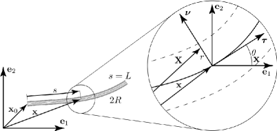
Figure 1: The virtual beam image and its coordinates system

The cartesian reference frame is $(\mathrm{\textbf{e}}_{1},\mathrm{\textbf{e}}_{2})$, the tangent and normal vectors are respectively $(\bm{\tau},\bm{\nu})$ and a point of the mean line is referred to as x (Eq. 1 and 2). There is no overlap, i.e. the points X are uniquely defined, since the local radius of curvature $1/|\gamma|$ is greater than the beam thickness R.

X $$= \mathrm{\textbf{x}}+r\bm{\nu}$$ (1)

x $$= \mathrm{\textbf{x}}_{0}+\int_{0}^{s}\bm{\tau}(\xi)\mathrm{d}\xi$$ (2)

In order to give a finite dimension to the problem, the curvature $\gamma(s)$ is described by a truncated series:

$$\gamma(s)=\sum_{n=0}^{N}A_{n}\tilde{\gamma}_{n}(\tilde{s}),$$ (3)

where $A_{n}$ are the coefficients of the series, $N$ its order, $\tilde{\gamma}_{n}(\tilde{s})$ the dimensionless basis functions and $\tilde{s}=s/L\in[0,1]$ the reduced curvilinear abscissa. By integration, the angles are given by:

$$\theta(s)=\theta_{0}+L\sum_{n=0}^{N}A_{n}\tilde{\theta}_{n}(\tilde{s})$$ (4)

in which

$$\tilde{\theta}_{n}(\tilde{s})=\int_{0}^{\tilde{s}}\tilde{\gamma}_{n}(\tilde{\xi})\mathrm{d}\tilde{\xi}.$$ (5)

Both $\tilde{\gamma}_{n}$ and $\tilde{\theta}_{n}$ depend only upon the choice of the series. They are estimated and stored prior to any computation. The set of parameters which must be determined are the magnitudes $A_{n}$ and $(\mathrm{\textbf{x}}_{0},\theta_{0}$).

The value of the gray levels $g(\mathrm{\textbf{X}})$ in the virtual image is chosen to be similar to that in the physical objects; it consists of a symmetrical function of the radius $g(\mathrm{\textbf{X}})=l(r)$ that continuously decreases from the mean line to the border:

$$2l(r)=1+\cos\left(\frac{\pi r}{R}\right).$$ (6)

The present method does not require that the virtual image be closely similar to the physical one. Both the width and the gray levels of the virtual beam may be very different from the physical ones; this will be illustrated by the examples.

3 Adjustment of the virtual beam to the physical picture

As shown in the previous section, for a given set of function $\tilde{\gamma}_{n}$, the shape of the virtual image G is fully described by the set of parameters $\mathbf{V}=\{\mathrm{\textbf{x}}_{0},\theta_{0},A_{n}\}$ (a pseudo-vector of dimension $N+4$ whose components are referred as $V_{k}$ hereafter in this section). In this section, we describe the method developed to find the optimal set $\mathbf{V}^{f}$, such that the beam image G falls best onto the image of the physical object that is contained in image F. Following [16], this is achieved by the minimization of the function $\Phi(V_{k})$:

$$\Phi=\iint_{D_{g}}\left(f-g\right)^{2}\mathrm{d}S$$ (7)

in which $f$ is the luminance of the physical image F and $\mathrm{d}S=(1-\gamma r)\mathrm{d}r\mathrm{d}s$ is the surface element. The domain $D_{g}$ is fully contained inside F so that $f$ is defined at any points. The optimal set $\mathbf{V}^{f}$ corresponds to the minimum of $\Phi$ then the condition $\mathrm{d}\Phi=(\partial\Phi/\partial V_{k})\mathrm{d}V_{k}=0$ must be fulfilled for any variation $\mathrm{d}V_{k}$ around $V_{k}^{f}$. Using Eq. (7) together with $\partial g/\partial V_{k}=\mathbf{grad}(g).\partial\mathrm{\textbf{X}}/\partial V_{k}$, this condition leads to:

$$\oint_{\partial D_{g}}\left((f-g)^{2}\,\mathrm{\textbf{n}}.\frac{\partial\mathrm{\textbf{X}}}{\partial V_{k}}\mathrm{d}V_{k}\right)\mathrm{d}l-2\iint_{D_{g}}\left(f-g\right)\left(\mathbf{grad}(g).\frac{\partial\mathrm{\textbf{X}}}{\partial V_{k}}\mathrm{d}V_{k}\right)\mathrm{d}S=0,$$ (8)

where $\partial D_{g}$ is the boundary of the domain $D_{g}$ i.e. the external boundary of the virtual beam, $\mathrm{d}l$ a differential line element and n a vector normal to the boundary and pointing outwards. Supposing that the iterative process is close to the solution, and that $R$ is slightly greater than the width of the physical object, this boundary $\partial D_{g}$ is located in the background of the physical image (we neglect the boundary sides at $s=0$ and $s=L$ as $R<<L$). Then, assuming that the background is uniform, $f|_{\partial D_{g}}$ (which represents the value of $f$ along the boundary $\partial D_{g}$) is constant. Furthermore, with the retained definition of $g$ (Eq. 6), $g|_{\partial D_{g}}=0$. Using the divergence theorem, we have:

$$\oint_{\partial D_{g}}(f-g)^{2}\,\mathrm{\textbf{n}}.\frac{\partial\mathrm{\textbf{X}}}{\partial V_{k}}\mathrm{d}V_{k}\quad\mathrm{d}l=(f|_{\partial D_{g}})^{2}\frac{\partial}{\partial V_{k}}\left(\iint_{D_{g}}\mathrm{div}(\mathrm{\textbf{X}})\mathrm{d}S\right)\mathrm{d}V_{k}$$ (9)

As $\mathrm{div}(\mathrm{\textbf{X}})=2$, the surface integral in Eq. (9) is constant (as $S=2RL$) and its derivative with respect to $V_{k}$ equals zero. Thus, assuming henceforth that the virtual beam boundary encloses the physical one and that the background of $f$ is uniform, Eq. 8 reduces to:

$$\iint_{D_{g}}\left(f-g\right)\left(\mathbf{grad}(g).\frac{\partial\mathrm{\textbf{X}}}{\partial V_{k}}\right)\mathrm{d}S=0.$$ (10)

The next step consists in considering the Taylor expansion of $g$ up to the first order:

$$g(V_{k}+\Delta V_{k})=g(V_{k})+\mathbf{grad}(g).\frac{\partial\mathrm{\textbf{X}}}{\partial V_{p}}\Delta V_{p}$$ (11)

which, when introduced in Eq. (10), gives:

$$\Delta V_{p}\iint_{D_{g}}\left(\mathbf{grad}(g).\frac{\partial\mathrm{\textbf{X}}}{\partial V_{k}}\right)\left(\mathbf{grad}(g).\frac{\partial\mathrm{\textbf{X}}}{\partial V_{p}}\right)\mathrm{d}S$$ (12)

$$= \iint_{D_{g}}\left(\mathbf{grad}(g).\frac{\partial\mathrm{\textbf{X}}}{\partial V_{k}}\right)(f-g)\mathrm{d}S,$$

This can be written as a matrix equation:

$$M_{kp}\Delta V_{p}=L_{k},$$ (13)

This equation represents a simple linear square matrix problem ($N+4$ dimension); its solution $\Delta V_{p}$ is used to update the shape of the virtual beam. The iterative process is repeated until the value of $\Phi$ decreases by less than a prescribed amount ($10^{-6}$) between two steps.

The term $\mathbf{grad}(g).\partial\mathrm{\textbf{X}}/\partial V_{k}$ is involved in both the expressions of $M_{kp}$ and $L_{k}$. From Eq. (6) and the beam geometry follows:

$$\mathbf{grad}(g)=l^{\prime}(r)\bm{\nu},$$ (14)

and, from Eq. (1):

$$\frac{\partial\mathrm{\textbf{X}}}{\partial V_{k}}=\frac{\partial\mathrm{\textbf{x}}}{\partial V_{k}}-r\frac{\partial\theta}{\partial V_{k}}\bm{\tau}.$$ (15)

The second term, collinear to $\bm{\tau}$, does not need to be computed as it is orthogonal to $\mathbf{grad}(g)$. The derivatives of $\partial\mathrm{\textbf{x}}/\partial V_{k}$ are obtained using Eq. (2) and (4):

$$\frac{\partial\mathrm{\textbf{x}}}{\partial x_{0,1}}=\mathrm{\textbf{e}}_{1},\frac{\partial\mathrm{\textbf{x}}}{\partial x_{0,2}}=\mathrm{\textbf{e}}_{2},\frac{\partial\mathrm{\textbf{x}}}{\partial\theta_{0}}=\int_{0}^{s}\bm{\nu}\mathrm{d}\xi,\frac{\partial\mathrm{\textbf{x}}}{\partial A_{n}}=L\int_{0}^{s}\tilde{\theta}_{n}\bm{\nu}\mathrm{d}\xi.$$ (16)

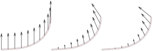
Figure 2: Examples of unitary displacement fields. From left to right: $\partial\mathrm{\textbf{x}}/\partial x_{0,2}$ (vertical translation), $\partial\mathrm{\textbf{x}}/\partial\theta_{0}$ (rotation) and $\partial\mathrm{\textbf{x}}/\partial A_{0}$ (uniform increase of the curvature).

The displacement of the virtual beam between two steps is close to $(\partial\mathrm{\textbf{X}}/\partial V_{k})\Delta V_{k}$ where the fields $\partial\mathrm{\textbf{X}}/\partial V_{k}$ represent unitary kinematic fields. Figure 2 shows an example of such fields (for clarity the fields are only represented at the mean line location, i.e. $\partial\mathrm{\textbf{x}}/\partial V_{k}$). They play the same role as the unitary displacement fields used in the DIC method [16, 17, 18].

The virtual image G is naturally discretized over the curvilinear frame $(s,r)$ that does not correspond to the square grid of image F. To avoid any loss of information, the mesh size of the virtual image is much smaller. The computation of the second member of Eq. (12) requires one to project the luminance field $f$ onto the mesh of G using, here, a cubic interpolation.

The overall length $L$ of the beam is currently not straightforwardly obtained by the VIC method. The end of the fiber is detected from the sharp variation of $\partial\Phi/\partial s$ which occurs at the point where the virtual beam exceeds the end of the fiber.

4 Determination of the initial conditions

It has been shown that the VIC method, detailed in the previous section, requires that the boundary of the virtual beam initially surrounds the image of the physical fiber. This section briefly describes the method used to determine these initial conditions.

The beam is first approximated by a sequence of straight segments. Their positions are given by a simplified VIC method in which the kinematic field is a single rotation around the first point of the segment. Finally the approximate shape is defined upon a collection of equally spaced points $\hat{\mathrm{\textbf{x}}}_{q}$ (with $0\leqslant q\leqslant Q$). This gives the segments angles $\hat{\theta}(\hat{s}_{q})$ where $\hat{s}_{q}$ are the curvilinear abscissae of points $\hat{\mathrm{\textbf{x}}}_{q}$. These data are used to define the set of initial parameters $V_{k}^{0}=\{\hat{\mathrm{\textbf{x}}}_{0},\hat{\theta}_{0},\hat{A}_{n}\}$ that will be used in the first step of the VIC computation. The first term, $\hat{\mathrm{\textbf{x}}}_{0}$, corresponds to the user-defined position of the initial point. The other terms are obtained by setting $A_{-1}=\theta_{0}/L$ and $\tilde{\theta}_{-1}(\tilde{s})=1$ in Eq. (4) which becomes:

$$\frac{\theta(s)}{L}=\sum_{n=-1}^{N}A_{n}\tilde{\theta}_{n}(\tilde{s}).$$ (17)

In particular, this equation applies to each value $\hat{\theta}(\hat{s}_{q})$ obtained from the previous approximative analysis, leading to:

$$\frac{\hat{\theta}(\hat{s}_{q})}{\hat{L}}=\sum_{n=-1}^{N}\hat{A}_{n}\tilde{\theta}_{n}\left(\frac{\hat{s}_{q}}{\hat{L}}\right),$$ (18)

where $\hat{L}=\hat{s}_{Q+1}$. From Eq. 5, the functions $\tilde{\theta}_{n}$ depend only on the series functions $\tilde{\gamma}_{n}$. Setting the order $N$ of the series such as $N+2=Q+1$ (the number of points $\hat{\mathrm{\textbf{x}}}_{q}$), this equation represents a linear square matrix system whose resolution gives the terms $\hat{A}_{n}$ (where $\hat{A}_{-1}=\hat{\theta}_{0}/\hat{L}$). This defines $V_{k}^{0}$ and the VIC computation may start at this order $(Q-1)$, or at a lower one if $V_{k}^{0}$ is truncated.

5 Example of applications of the VIC method

This section describes two examples especially chosen to illustrate, from a practical point of view, the different steps involved in the technique. The first example (Sec. 5.1) validates the accuracy of the method for a simple geometry; the second (Sec. 5.2) demonstrates its robustness in the case of a curled shape and a low quality image.

5.1 The cantilever beam

We proceeded to a simple experiment of a cantilever (clamped at one end) straight bar, bent under its own weight (Fig. 3a).

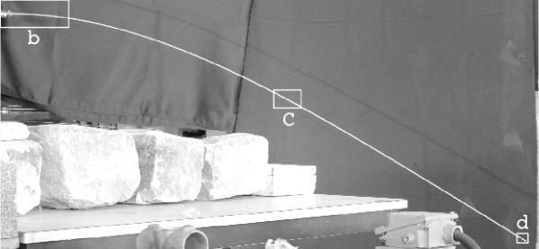
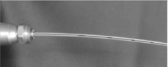
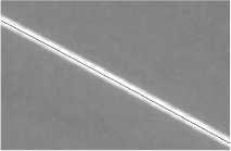
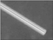
(a) (b) (c) (d)

Figure 3: (a) Aluminium bar bending under its own weight and identified mean line (white). (b-d) Magnified views of regions (b) close to the chuck, (c) midway along the bar and (d) at the tip. Solid black line: mean line obtained by the VIC method for a Legendre series of order 3.

The 2017-T4 aluminium bar has a length of $2459$ mm and a radius of $4.95$ mm. It is left free to bend under its own weight with one of its ends clamped in an horizontal chuck (Fig. 3b). A black curtain was placed in the back of the device in order to obtain a good intensity contrast and an uniform background (the latter condition is detailed in Sec. 3). A single light has been positioned close to the camera in order to illuminate equally both sides of the rod (in order to have a symmetrical luminance function $f(r)$). Once the bar is at rest (this may take a few minutes) an high resolution picture is captured using a Nikon D300 digital camera. This image (cropped from the original one) has $3897\times 1841$ pixels. The field of view represents $2.33\times 1.09$ m² in the focal plane.

For this image, we used Legendre series for the functions $\tilde{\gamma}_{n}$ in Eq. (3). The Fourier series used in Sec. 5.2 provides similar results, but an higher order is needed. The Legendre series, in their shifted version ($\tilde{s}\in[0..1]$), can be written as:

$$\tilde{\gamma}_{n}=P_{nk}\tilde{s}^{k},$$ (19)

where $k\in[0,N]$ and with [19]:

$$P_{nk}=(-1)^{(n+k)}\left(\begin{array}[]{c}n\\ k\end{array}\right)\left(\begin{array}[]{c}n+k\\ k\end{array}\right),$$ (20)

in which the parenthesis refers to combination formulas. Yet, for our particular example, because of the small contrast between the chuck maintaining the bar and the bar itself (see Fig. 3b), the abscissa $x_{0,1}$ was fixed so as to avoid any unwanted inclusion of the clamping device onto the virtual beam. The set of shape parameters (introduced in Sec. 3) reduces to $V_{k}=\{x_{0,2},\theta_{0},A_{n}\}$.

Fig. 3 shows the result of the identification for an order $N=3$: the mean line of the virtual beam perfectly follows the middle of the aluminium bar along its full length. Due to its structure, the VIC method is not influenced by large and illuminated objects present in the foreground of the picture (like the stones on the bottom left of Fig. 3a). The virtual beam diameter was set at $20$ pixels (the physical bar diameter is around 10 pixels). The virtual beam mesh has $61\times 8634$ points (approximatively three times thinner than the image grid). The total time required for the computation was about $3$ seconds per iteration using a 2.8 GHz dual-core computer and an algorithm implemented on Matlab.

We now compare these results to the prediction of the elastic beam theory [15]. According to it, the flexural moment $M(s)$, given by static equilibrium, is proportional to the local curvature:

$$M(s) = \int_{s}^{L}\rho\left(x_{1}(\xi)-x_{1}(s)\right)\mathrm{d}\xi,$$ (21)

$$M(s) = E\frac{\pi R^{4}}{4}\gamma(s),$$ (22)

$$\theta(0) = 0,$$ (23)

where the abscissa $x_{1}$ is measured along the horizontal axis. This system is solved using a numerical iterative method and the physical properties $\rho=2700$ g/cm³ and $E=72$ GPa [20]. The Young modulus was confirmed by a three-point bending test performed on the actual specimen, leading to $72.6$ GPa.

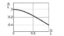
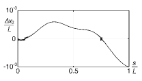
(a)                                                      (b)

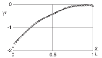
(c)                                                      (d)

Figure 4: Comparison between the beam theory (solid line) and the VIC method (circles). (a) Displacement. (b) Discrepancy between the two determinations of the vertical displacement. (c) Angle (radians). (d) Curvatures.

Fig. 4a shows that the results given by the beam theory match very well the measurements from the VIC method, in term of displacement in the $x_{1}$ (horizontal) $x_{2}$ (vertical) plane. Fig. 4b presents a magnified view of the same result and only small differences are observed: the mean quadratic vertical distance between the two solutions is approximatively of $2$ pixels (i.e. $1.2$ mm). A similar discrepancy has been observed in a second experiment in which the chuck was rotated by an half turn. Figs. 4c and 4d demonstrate that the VIC method determines correctly the slopes and curvatures. In particular, both the initial slope $\theta(s=0)=0$ and the final curvature $\gamma(s=L)=0$ are correctly determined (note that their value were not imposed by the Legendre polynomial sequence used).

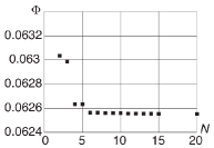
Figure 5: Dependence of the final value of the correlation function $\Phi$ on the order $N$.

The choice of the order $N$ results from a classical compromise between simplicity and accuracy. An order too low (here $N=1$) may lead to a loss of correlation between F and G (the boundary $\partial D_{g}$ does not enclose anymore the image of the object). Increasing the order monotonically decreases the value of the correlation function (Fig. 5). When the order becomes too high (for $N>12$ in this example) the matrix $M_{kp}$ in Eq. (13) becomes ill-defined while the level of $\Phi$ asymptotically reaches a minimum value.

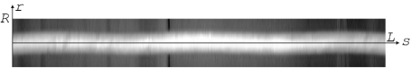
(a)

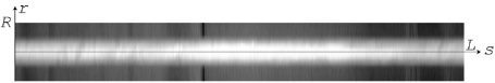
(b)

Figure 6: a) and b) : the physical beam image in the unwrapped coordinates of the virtual beam for $N=3$ and $N=8$.

A visual comparison of the results obtained for two different values of $N$ is displayed in Figs. 6a and 6b. They represent the physical image in the reference frame $(s,r)$ of the virtual beam (represented unwrapped for clarity). In the case of an ideal correlation, whatever the shape of the fiber, this figure should be symmetrical with respect to the (straight) mean line. Because of the magnification along the $r$ axis, one can see that the image in Fig. 6a obtained for a low order $N=3$ is slightly wavy while the image in Fig. 6b obtained for $N=8$ is perfectly symmetrical. The inhomogeneities of the illumination and of the background are visible but do not influence the final result.

5.2 The fiber transported by a fluid flow in a fracture

This second example illustrates the robustness of the technique with regard to the quality of the physical image F and to the complex shape of the object.

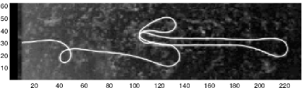
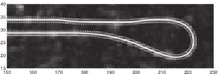
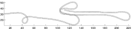
(a) (b) (c) (d)

Figure 7: Fiber transported by a fluid flow in a fracture (units are in pixels). (a) Physical image. (b) Same image and identified mean line (white line). (c) Detailed view: identified mean line (white line) and border of the virtual image (white dots). (d) Virtual beam.

This example deals with the transport of a fiber by a flow fluid in a transparent fracture made of two rough surfaces [21] (Fig. 7). Because of the fracture roughness, the free space has a complex geometry leading to a disordered flow velocity field. As a result, when a fiber of diameter (0.3 mm) close to the fracture aperture (0.75 mm) is inserted into the fracture, it is subject to spatially variable forces from the fluid resulting in strong deformations of the thread. Fiber transport is only possible at large fluid velocities so that images need to be captured at high rates with a poor light intensity contrast.

Several attempts using thresholding operations and spline interpolations were made to extract the center line of the fiber but none of them gave a solution well fitted to the whole profile of the fiber at a given time. This was especially obvious in situations of large deformation with buckling. The noise level of the picture was a major problem for thresholding methods (the light intensity of spots in the background is close to that of the pixels corresponding to the fiber).

The experimental pictures were them reanalyzed using the VIC method. A Fourier series containing $N=100$ terms was necessary to describe this complex shape (the previously used Legendre series lead to numerical problems due to large values of $P_{nk}$ in Eq. 20). Fig. 7c shows that the fiber diameter is close to one pixel then a slightly larger width, $R=1$ pixel, has been selected for the virtual beam. Similarly to previous example, the abscissa $x_{0,1}$ of the first point (on the left of Fig. 7a) has been fixed in order to avoid unwanted edge effects.

The Fig. 7 clearly shows that the VIC method gives an accurate estimation for the central line of the fiber. Despite the small radius of the object and the high noise level, the central line collapses everywhere onto the fiber. Wide meanders as well as small deviations from a straight line are perfectly followed. Moreover, even the loops of the fiber can be extracted by this method.

6 Conclusion and discussion

The Virtual Image Correlation method allows one to identify precisely the shape of a fiber from its image. The virtual beam fully encloses the physical image of the fiber so that all the information contained in it is used (and not only its brightest pixels); this feature contributes to the precision of the method. Furthermore, pixels outside of the definition domain are not used: this speeds up the computation and makes it insensitive to possible artefacts in the background. The method can deal with noisy images and strongly curved fibers; it can already be used in various domains, from biology to mechanical engineering. The analytical identification of the curvatures given by the VIC provides informations on the mechanical state of the fiber: it is possible to identify its flexural properties from the knowledge of external forces. Conversely, if the mechanical parameters are known, one can compute (using an inverse problem approach), the external forces acting on the fiber.

From a theoretical point of view, it would be interesting to include the length of the fiber in the optimization process. The examples provided in the present paper use either Fourier or Legendre series decompositions for the representation of the mean line. Other series such as the Chebyshev polynomials or other functions used for Computed Aided Design (Bézier curves, splines…) may also be used. Following [22, 16], if the method is used for identifying the mechanical properties of the fiber, one should define the main term of the series from the theoretical beam equation.

Time sequences will also be considered: the variation of images with time allow one to increase the precision of the analysis and to study the dynamic of the buckling process. Three-dimensional analysis is also envisaged and will use at least two pictures taken from different angles of view.

The VIC method can also be applied to images of other curvilinear shapes (non fiber objects) in various scientific domains in which the curvature has a major role, for example thermal or diffusion fronts in fluid mechanics, chemistry… It may also be useful in the ”pure” image processing field in some case of line or pattern recognition. With a slight modification of the virtual beam luminance definition (a step shape), the method may also be applied to edge detection problems.

References

- [1] Clarence R. Robbins. Chemical and Physical Behavior of Human Hair. Springer Verlag, Berlin, fourth edition, 2002.
- [2] O L Forgacs and S G Mason. Particle motions in sheared suspensions: X. Orbits of flexible threadlike particles. Journal of Colloid Science, 14:473–491, 1959.
- [3] S H Okazawa, R Ebrahimi, J Chuang, R N Rohling, and S E Salcudean. Methods for segmenting curved needles in ultrasound images. Medical Image Analysis, 10(3):330–342, 2006.
- [4] JH Shin, L Mahadevan, PT So, and P Matsudaira. Bending stiffness of a crystalline actin bundle. Journal of Molecular Biology, 337(2):255–261, 2004.
- [5] W R DiLuzio, L Turner, M Mayer, P Garstecki, D B Weibel, H C Berg, and G M Whitesides. Escherichia coli swim on the right-hand side. Nature, 435:1271–1274, 2005.
- [6] R Dreyfus, J Baudry, ML Roper, M Fermigier, H A Stone, and J Bibette. Microscopic artificial swimmers. Nature, 437:862–865, 2005.
- [7] P Garstecki, P Tierno, D B Weibel, F Sagués, and G M Whitesides. Propulsion of flexible polymer structures in a rotating magnetic field. Journal of Physics: Condensed Matter, 21, 2009.
- [8] Stephen R. Aylward and Elizabeth Bulitt. Initialisation, noise, singularities, and scale in height ridge traversal for tubular object. IEEE Transactions on Medical Imaging, 21(2):61–75, 2002.
- [9] Thomas Deschamps and Laurent D. Cohen. Fast extraction of minimal paths in 3D images and application to virtual endoscopy. Medical Image Analysis, 5(4):281–299, 2001.
- [10] Daniel Mueller and Anthony Maeder. Robust semi-automated path extraction for visualising stenosis of the coronary arteries. Computerized Medical Imaging and Graphics, 32(6):463–475, 2008.
- [11] L Xu, E Oja, and P Kultanen. A new curve detection method: randomized Hough transform (RHT). Pattern Recognition Letters, 11(5):331–338, 1990.
- [12] Wilson C.Y. Lam, Kelvin S.Y. Yuen, and Dennis N.K. Leung. Fourier parameterization provide uniform bounded Hough Space, volume 719 of Lecture Notes in Computer Science, pages 183–190. Springer Verlag, Berlin, 1993.
- [13] Peter A Toft. Using the generalized radon transform for detection of curves in noisy images. Proceedings of the IEEE ICASSP-96 Conference, 4:2219–2222, 1996.
- [14] Vicent Caselles, Ron Kimmel, and Guillermo Sapiro. Geodesic active contours. International Journal of Computer Vision, 22(1):61–79, 1997.
- [15] S Timoschenko. Schwingungsprobleme der technik. Springer Verlag, Berlin, 1932.
- [16] François Hild and Stéphane Roux. Digital image correlation: from displacement measurement to identification of elastic properties - a review. Strain, 42(2):69–80, 2006.
- [17] François Hild and Stéphane Roux. Measuring stress intensity factors with a camera: integrated digital image correlation (I-DIC). Comptes Rendus de Mécanique, 334:8–12, 2006.
- [18] Julien Rethore, Stéphane Roux, and François Hild. From pictures to extended finite elements: extended digital image correlation (X-DIC). Comptes Rendus de Mécanique, 335(3):131–137, 2007.
- [19] Murray R. Spiegel, John Liu, and Seymour Lipschutz. Mathematical Handbbok of Formulas and Tables. McGraw-Hill, 1999.
- [20] J. Lemaitre and J L Chaboche. Mécanique des matériaux solides. Dunod, Paris, 1988.
- [21] M V D’Angelo, B Semin, G Picard, M Poitzsch, J P Hulin, and H Auradou. Single fiber transport in a fracture slit: influence of the wall roughness and of the fiber flexibility. Submitted to Transport in Porous Media, 2009.
- [22] Michel Grédiac, Evelyne Toussaint, and Fabrice Pierron. Special virtual fields for the direct determination of material parameters with the virtual fields method. 1-Principle and definition. International Journal of Solids and Structures, 39(10):2691–2705, 2002.