Theoretical values of convective turnover times and Rossby numbers for solar-like, pre-main sequence stars

Abstract

Context. Magnetic fields are at the heart of the observed stellar activity in late-type stars, and they are presumably generated by a dynamo mechanism at the interface layer (tachocline) between the radiative core and the base of the convective envelope.

Aims. Since dynamo models are based on the interaction between differential rotation and convective motions, the introduction of rotation in the ATON 2.3 stellar evolutionary code allows for explorations regarding a physically consistent treatment of magnetic effects in stellar structure and evolution, even though there are formidable mathematical and numerical challenges involved.

Methods. As examples of such explorations, we present theoretical estimates for both the local convective turnover time ($\tau_{\rm c}$), and global convective times ($\tau_{\rm g}$) for rotating pre-main sequence solar-type stars, based on up-to-date input physics for stellar models. Our theoretical predictions are compared with the previous ones available in the literature. In addition, we investigate the dependence of the convective turnover time on convection regimes, the presence of rotation and atmospheric treatment.

Results. Those estimates, as opposed to the use of empirically derived values of $\tau_{\rm c}$ for such matters, can be used to calculate the Rossby number $Ro$, which is related to the magnetic activity strength in dynamo theories and, at least for main-sequence stars, shows an observational correlation with stellar activity. More important, they can also contribute for testing stellar models against observations.

Conclusions. Our theoretical values of $\tau_{\rm c}$, $\tau_{\rm g}$ and $Ro$ qualitatively agree with those published by Kim & Demarque (1996). By increasing the convection efficiency, $\tau_{\rm g}$ decreases for a given mass. FST models show still lower values. The presence of rotation shifts $\tau_{\rm g}$ towards slightly higher values when compared with non-rotating models. The use of non-gray boundary conditions in the models yields values of $\tau_{\rm g}$ smaller than in the gray approximation.

1 Introduction

Magnetic activity in solar-type stars encompasses a variety of phenomena, such as star spots, activity cycles, heated outer atmospheres, X-ray emission, and many others. The driving mechanism for this activity is generally attributed to a dynamo that results from the interaction between rotation and convective motions in the star’s outer envelope. Theoretical work by a number of researchers indicates that for main-sequence, solar-type stars the field is generated and amplified at the tachocline, the thin layer of differential rotation between the convection zone and the nearly rigidly rotating radiative interior. For stars of a spectral type ranging from mid-F to early-M dwarfs, rotation and activity are thought to be controlled by this process, also called an $\alpha$$-$$\Omega$ dynamo (Mohanty & Basri,, 2003). Its efficiency is strongly dependent on the rotation rate and convective timescales. Young and rapidly rotating stars are, in general, very active. Specific models of dynamo theory, such as the $\alpha$$-$$\Omega$ type, have been successful in explaining the qualitative features of solar activity (Weiss & Tobias,, 2000).

Activity is strongly correlated with rotation velocity in the mid-F to mid-M dwarfs; it increases rapidly with the projected velocity, $v\sin i$, then saturates above some threshold velocity ($\sim$ 10 km/s). This relationship is evident only down to K types; as we go from M to M6 types the rotation-activity connection becomes less clear. Mohanty & Basri, (2003) analyzed rotation velocities and chromospheric H${\alpha}$ activity, derived from high-resolution spectra, in a sample of mid-M to L field dwarfs. They found that, in the spectral type range M4-M8.5, the saturation-type rotation-activity relation is similar to that in earlier types, but the activity saturates at a significantly higher velocity in the M5.5-M8.5 dwarfs than in the M4-M5 ones; this may result from a change in the dynamo behavior in later spectral types.

For fully convective stars, such as pre-main sequence late-type stars, this theory cannot be readily applied, as they miss the tachocline. However, since magnetic indicators such as active regions and strong flaring have also been reported for those stars, dynamo mechanisms operating on the full convection region have also been proposed (e.g. Durney et al.,, 1993).

On the other hand, observations of stellar activity in solar-type stars have shown a very tight relationship between chromospheric Ca II H-K flux and the Rossby number $Ro=P_{\rm rot}/\tau_{\rm c}$, where $P_{\rm rot}$ is the rotation period and $\tau_{\rm c}$ is the local convective turnover time. The Rossby number plays an important role in dynamo models, being related to the dynamo number $D=Ro^{-2}$ which, in turn, is related to the growth rate of the field. For solar-type stars, since $\tau_{\rm c}$ cannot be directly measured, $Ro$ is generally computed through a polynomial fit of $\tau_{\rm c}$ to the B$-$V color index. For example, Noyes et al., (1984) give $\tau_{\rm c}{\rm(B-V)}$ as a theoretically-derived convective overturn time, calculated assuming a mixing length to scale height ratio $\alpha\sim 2$.

For pre-main sequence stars, Rossby numbers have been used to study the relationship between the X-ray emission and magnetic fields (e.g. Flaccomio et al.,, 2003; Feigelson et al.,, 2003). In this case, however, no clear relationship between activity and rotation is seen, as in the case of main-sequence stars, and one has to resort to evolutionary models for estimating Rossby numbers.

Though current stellar evolutionary codes are not yet able to deal with magnetic fields, a first step towards this direction is the introduction of rotation on the models, as it is a key component of stellar dynamos. This is the case of the ATON 2.3 evolutionary code, in which both rotation and internal angular momentum redistribution have been introduced. Such capabilities allow us to make some exploratory work towards a future version that can handle magnetic field generation from first principles.

In this work we computed convective turnover times and Rossby numbers for a range of rotating low-mass stellar models, and discuss their behavior with time from the pre-main sequence to the zero-age main sequence. Our results are mainly compared with those found by Kim & Demarque, (1996), who provided the first self-consistent local and global convective turnover times and purely theoretical Rossby numbers (but see also Jung & Kim, 2007).

In Sect. 2 we describe the stellar evolutionary code used in this work (ATON code) as well as the specific inputs adopted for the present calculations. Results on Rossby number calculations are discussed in Sect. 3. The impact of other physical phenomena (like convection, rotation and atmospheric boundary conditions) is analyzed in Sect. 4. In Sect. 5 we present a simple application of our calculations to stars from the IC 2602 open cluster. Our conclusions are given in Sect. 6.

2 Input physics

The ATON 2.3 code has many updated and modern features regarding the physics of stellar interiors, of which a full account can be found in Ventura et al., 1998b . Some of its most important features are: most up-to-date OPAL (Iglesias & Rogers,, 1993) opacities, supplemented by those of Alexander & Ferguson, (1994) for lower (T $<6000K$) temperatures; diffusive mixing and overshooting; and convection treatment under either the mixing length theory (MLT) or the Full Spectrum of Turbulence (FST) from Canuto & Mazzitelli, (1991, 1992) and Canuto et al., (1996). In addition to the standard gray atmosphere boundary conditions, the ATON code can also handle non-gray atmospheric integration based on the models by Heiter et al., (2002); Hauschildt et al., (1999); Allard et al., (2000) as described in Landin et al., (2006).

The structural effects of rotation were implemented in the ATON code according to the Kippenhahn & Thomas, (1970) method, as improved by Endal & Sofia, (1976). Although the ATON code can handle the chemical mixing of species by using a diffusive approach (microscopic diffusion), the models presented here use instantaneous mixing, which is a good approximation for pre-main sequence stars (Ventura & Zeppieri, 1998a, ). We account also for the mixing caused by rotational instabilities (Endal & Sofia,, 1978), including dynamical instabilities (Solberg-Høiland and dynamical shear) and secular instabilities (secular shear, Goldreich-Schybert-Fricke and meridional circulation). Angular momentum redistribution in radiative regions was modeled through an advection-diffusion equation based on the framework of Chaboyer & Zahn, (1992) and Zahn, (1992). Angular momentum losses in the star’s external layers due to magnetized stellar winds are also taken into account in the form of a boundary condition at the surface. We adopted the prescription used in Chaboyer et al., (1995) with a “wind index” $n=1.5$, which reproduces well the Skumanich, (1972) law $v\propto t^{-1/2}$:

$${{\partial J}\over{\partial t}}\!=\!K\!\left(\!{R\over R_{\odot}}\!\right)^{\!2-n}\!\!\left(\!{M\over M_{\odot}}\!\right)^{\!-\frac{n}{3}}\!\!\left(\!{\dot{M}\over 10^{-14}}\!\right)^{\!1-\frac{2n}{3}}\!\!\!\omega^{1+\frac{4n}{3}},\hskip 8.5359pt\omega<\omega_{\rm crit},$$ (1)

$${{\partial J}\over{\partial t}}\!=\!K\!\left(\!{R\over R_{\odot}}\!\right)^{\!2-n}\left(\!{M\over M_{\odot}}\!\right)^{\!-\frac{n}{3}}\left(\!{\dot{M}\over 10^{-14}}\!\right)^{\!1-\frac{2n}{3}}\!\!\!\omega\omega_{\rm crit}^{\!\frac{4n}{3}},\hskip 8.5359pt\omega\geq\omega_{\rm crit},$$ (2)

where $\omega_{\rm crit}$ introduces a critical rotation level at which the angular momentum loss saturates (set to $5\,\Omega_{\odot}$ in our models, where $\Omega_{\odot}$ is the current solar surface rotation rate). The constant $K$ in our models was calibrated by adjusting a 1 M_⊙ model so that its surface velocity matches the current solar rotation rate at the equator. $\dot{M}$ is the mass loss rate, which enters in Eqs. (1) and (2) in units of $10^{-14}M_{\odot}\,yr^{-1}$, and which we set to 1.0.

For the initial rotation rates, we adopt the relation between initial angular momentum (J_in) and stellar mass obtained from the corresponding mass-radius and mass-moment of inertia relations from Kawaler, (1987):

$$J_{\rm in}=1.566\times 10^{50}\left({M\over M_{\odot}}\right)^{0.985}\quad{\rm g}\,{\rm cm}^{2}\,{\rm s}^{-1}.$$ (3)

For more details about the treatment given to rotation in the ATON code, see Mendes, (1999) and Mendes et al., (1999, 2003).

3 Rossby number calculations

Convective turnover times and Rossby numbers were computed for models ranging from 0.6 to 1.2 M_⊙ (in 0.1 M_⊙ increments) with solar chemical composition. For ease of comparison with a previous work by Kim & Demarque, (1996), who provided theoretical calculations of Rossby numbers for pre-main sequence stars, convection was treated according to the MLT, with the free parameter $\alpha$ set to 1.5 (which fits the solar radius at the solar age for a gray atmosphere, non-rotating model). Convection treatment and boundary conditions considerably affect the calculations of global convective turnover times and, consequently, the Rossby numbers (see Sect. 4.1). Rotation was modeled according to rigid body law in convective zones and local conservation of angular momentum in radiative regions (Mendes et al.,, 2003).

We followed the evolution of local and global convective turnover times (to be defined shortly) and Rossby numbers during the pre-main sequence for 0.6-1.2 M_⊙ stars and tabulated them together with the corresponding evolutionary tracks. Table 1 presents the 1 M_⊙ models as an example of such tables. Column 1 gives the logarithm of stellar age (in years); Col. 2 the logarithm of stellar luminosity (in solar units); Col. 3 the logarithm of effective temperature (in K); Col. 4 the logarithm of effective gravity (in cgs); Col. 5 the logarithm of local convective turnover time (in seconds); Col. 6 the global convective turnover time (in days); and Col. 7 the Rossby number.

Table 1: Pre-main sequence evolutionary tracks (including $\log\tau_{c}$, $\log\tau_{g}$ and $Ro$) for 1 M_⊙ star^a.

${\log Age\atop{\rm(years)}}$	$\log\frac{L}{L_{\odot}}$	${\log T_{\rm eff}\atop{\rm(K)}}$	$\log g\atop{\rm(cgs)}$	$\log\tau_{c}\atop{\rm(seconds)}$	$\tau_{g}\atop\rm{(days)}$	$Ro$
6.2324	0.1468	3.6524	3.855	6.3275	766.6288	0.1436
6.4053	0.0217	3.6513	3.976	7.1018	488.2106	0.0183
6.5840	$-$0.1029	3.6499	3.095	7.0810	369.1187	0.0146
6.7666	$-$0.2172	3.6494	4.207	7.0074	291.4590	0.0131
6.9324	$-$0.2965	3.6522	4.297	6.9087	227.1363	0.0129
7.0786	$-$0.3278	3.6606	4.362	6.7949	179.1020	0.0135
7.2016	$-$0.2987	3.6775	4.401	6.6878	134.8216	0.0145
7.2978	$-$0.2231	3.6999	4.415	6.5727	99.6126	0.0165
7.3740	$-$0.1262	3.7232	4.411	6.4301	72.7130	0.0204
7.4394	$-$0.0387	3.7445	4.409	6.2546	53.4192	0.0269
7.5214	$-$0.0924	3.7525	4.494	6.1771	41.6650	0.0232
7.9918	$-$0.1590	3.7461	4.536	6.1942	46.0585	0.0212
9.0247	$-$0.1138	3.7531	4.518	6.1821	42.4793	0.2593
9.3023	$-$0.0862	3.7553	4.499	6.1523	41.0925	0.7916
9.4669	$-$0.0580	3.7572	4.479	6.1598	39.4493	1.0789
9.5829	$-$0.0288	3.7591	4.457	6.1303	38.1493	1.4206
9.6573	$-$0.0040	3.7605	4.438	6.1369	38.0850	1.5989
9.6980	0.0119	3.7612	4.425	6.1409	37.5359	1.7020
9.7644	0.0428	3.7624	4.399	6.1102	36.8616	2.0771
9.8211	0.0754	3.7634	4.370	6.1166	36.2118	2.3108
aThe complete version of the table, including seven tracks for all the masses of Table 2, will be available in electronic form.

Figure 1 depicts the rotation period as a function of age for all models, and shows the typical spin-up during contraction followed by the longer phase of continuous spin-down.

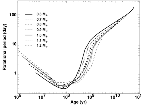
Figure 1: Rotation period plotted against age, for each model mass.

For the 1 M_⊙ model, this results in an initial velocity of nearly 3 km s^-1 at the beginning of the Hayashy phase; this is about one order of magnitude below the value used by Kim & Demarque, (1996). When calculating convective overturn times, one must make an arbitrary assumption about where in the convection zone the dynamo is operating. This assumption significantly affects the value of $\tau_{\rm c}$, since it is strongly dependent on the depth. In this work, we follow Gilliland, (1986) and calculate the “local” convective turnover time $\tau_{\rm c}$ at a distance of one-half the mixing length, $\alpha\,H_{\rm P}/2$, above the base of the convection zone. Its value is computed through the equation $\tau_{\rm c}=\alpha\,H_{\rm P}/v$, where $v$ is the convective velocity. It should be noted, however, that there is no agreement in the literature regarding the precise location where $\tau_{\rm c}$ should be computed; Montesinos et al., (2001), for example, calculate it at distance of $0.95\,H_{\rm P}$ above the base of convective zone, with $H_{\rm P}$ taken as its value at the base of the convection zone.

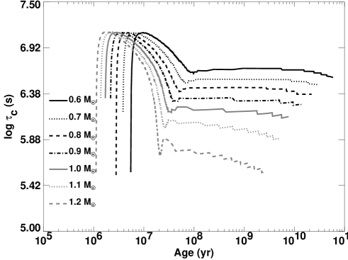
Figure 2: “Local” convective turnover time as a function of age for all models.

Figure 2 shows the time evolution of the local convective turnover time (in seconds). For a given mass, it decreases during the Hayashy contraction and reaches its minimum when the contraction stops. After that, $\tau_{\rm c}$ remains constant until the stars reach a main sequence configuration.

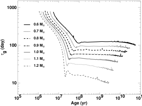
Figure 3: “Global” convective turnover time as a function of age for each model mass.

However, most relevant for our purposes are Figs. 3 and 4, which show the profiles of the “global” convective turnover time and the “dynamo number”, $Ro^{-2}$, respectively, as functions of age. The global convective turnover time ($\tau_{\rm g}$) is defined as

$$\tau_{\rm g}=\int_{R_{b}}^{R_{\star}}{dr\over v},$$ (4)

where $R_{b}$ is the radius at the bottom of the convective zone, $R_{\star}$ is the stellar radius and $v$ is convective velocity.

Figure 3 shows that $\tau_{\rm g}$ follows the same behavior as the local convective turnover time, also decreasing substantially during contraction to the zero-age main sequence and, after that, remaining nearly constant and depending only on the mass. As in Kim & Demarque, (1996), the local convective turnover time behaves like $\tau_{\rm g}$ except for a scaling factor, because the convective turnover timescale is weighted towards the deepest part of the convection zone, where the shortcomings of the mixing length approximation are less important. With regard to $Ro^{-2}$, it is seen from Fig. 4 that it follows $\tau_{\rm c}$ during contraction but, after that, decreases as expected since the rotation period also increases.

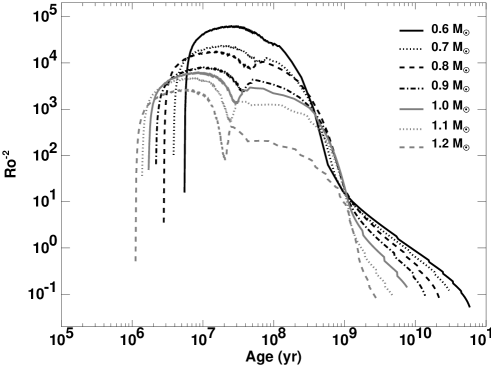
Figure 4: The dynamo number as a function of age for each model mass.

By using the evolutionary tracks, we constructed a set of isochrones for the ages of 0.2, 0.5, 0.7, 1.0, 2.0, 4.55 (solar age), 10 and 15 Gyr. In Table 2 we list their characteristics such as stellar mass in solar masses (Col. 1); logarithm of the effective temperature, in Kelvin (Col. 2); logarithm of the stellar luminosity, in cgs (Col. 3); global convective turnover time, in days (Col. 4); dynamo number (Col. 5); and the rotation period, in days (Col. 6).

In Fig. 5 we show a plot of the global and local convective turnover times versus $\log(T_{\rm eff})$ for each age. Isochrones for the global convective turnover time versus period are shown in Fig. 6. The highest point of each curve corresponds to the lowest mass. For a given mass, $\tau_{\rm g}$ varies slightly with the period. For a given period and age, the global convective turnover time depends on stellar mass.

Table 2: Isochrones for all models.

Mass			$\tau_{\rm g}$		Rotation
(M⊙)	$\log$ (Teff)	$\log$ (L/L⊙)	(days )	$Ro^{-2}$	Period (d)
0.2 Gyr
0.60	3.6148	$-$1.13663	121.1802	8627.8177	0.5581
0.70	3.6508	$-$0.85884	93.8181	4711.2816	0.5913
0.80	3.6878	$-$0.60171	77.0336	4601.9900	0.4777
0.90	3.7218	$-$0.36391	57.9367	2093.6635	0.5387
1.00	3.7480	$-$0.14791	43.8863	1643.1720	0.4534
1.10	3.7695	0.05200	30.5734	875.9235	0.4187
1.20	3.7908	0.23895	14.8697	136.2882	0.5509
0.5 Gyr
0.60	3.6148	$-$1.12952	121.9241	365.2809	3.3443
0.70	3.6511	$-$0.85206	94.4531	364.8090	2.2956
0.80	3.6898	$-$0.59006	73.5144	569.3372	1.3836
0.90	3.7241	$-$0.35056	57.1289	426.6247	1.2034
1.00	3.7511	$-$0.13146	42.1241	365.2252	0.9081
1.10	3.7734	0.07207	28.4896	268.6685	0.7299
1.20	3.7938	0.26043	13.4697	42.9852	0.8630
0.7 Gyr
0.60	3.6146	$-$1.12785	122.7990	45.4688	8.1315
0.70	3.6512	$-$0.84948	93.9007	69.1059	5.3534
0.80	3.6903	$-$0.58622	73.8996	130.3651	2.8620
0.90	3.7248	$-$0.34541	56.8609	115.0898	2.1514
1.00	3.7521	$-$0.12448	42.0428	122.1356	1.5846
1.10	3.7748	0.08167	26.7088	92.5457	1.1571
1.20	3.7950	0.27275	12.7590	23.7916	1.0832
1 Gyr
0.60	3.6145	$-$1.12602	123.9869	15.6947	13.7087
0.70	3.6514	$-$0.84667	93.3632	15.1359	10.3630
0.80	3.6908	$-$0.58179	74.2237	20.3958	7.2070
0.90	3.7255	$-$0.33908	56.5470	19.0868	5.2591
1.00	3.7530	$-$0.11547	41.4909	21.0411	3.8355
1.10	3.7760	0.09436	25.8848	15.9412	2.8429
1.20	3.7962	0.28993	11.7507	9.2329	1.6338
2 Gyr
0.60	3.6149	$-$1.11995	124.0207	5.5953	22.8118
0.70	3.6523	$-$0.83796	93.6465	4.6988	18.5225
0.80	3.6925	$-$0.56838	74.4090	4.3392	15.5263
0.90	3.7275	$-$0.31932	56.1457	2.8531	13.6315
1.00	3.7553	$-$0.08640	41.0063	1.6047	12.9745
1.10	3.7783	0.13614	24.9018	0.6022	12.7151
1.20	3.7979	0.34593	10.3207	0.2400	9.0570
4.55 Gyr
0.60	3.6163	$-$1.10689	123.5031	2.1587	36.6458
0.70	3.6548	$-$0.81720	93.2665	1.7031	30.6947
0.80	3.6970	$-$0.53436	71.9753	1.3278	27.0554
0.90	3.7327	$-$0.26633	56.5844	0.8790	24.8868
1.00	3.7605	$-$0.00376	38.2314	0.3903	25.3930
1.10	3.7807	0.25629	21.7054	0.1036	27.8899
10 Gyr
0.60	3.6196	-1.08068	121.1537	0.8633	55.7920
0.70	3.6610	-0.77093	90.9166	0.6376	47.6948
0.80	3.7070	-0.45253	69.9406	0.4504	43.8041
0.90	3.7428	-0.12491	51.0290	0.2126	44.6414
15 Gyr
0.60	3.6228	$-$1.05579	119.3184	0.5619	69.1454
0.70	3.6674	$-$0.72295	89.8339	0.3972	60.0909
0.80	3.7163	$-$0.35931	66.2647	0.2143	58.7162

Figure 5: The global and local convective turnover times as a function of effective temperature and age.

Figure 6: The global convective turnover time as a function of rotation period and age.

Figure 7 shows the rotation period versus $\log(T_{\rm eff})$. In that figure the rightmost points (those with the lowest temperatures) correspond to the lowest mass considered, namely 0.6 M_⊙. We recall that in our rotating models convective regions are modeled by assuming rigid body rotation, while radiative regions rotate according to local conservation of angular momentum.

In Fig. 8 we plotted the inverse square of the Rossby number versus the rotation period. The lowest point of each line represents the highest mass.

Figure 7: Rotation period as a function of effective temperature and age.

Figure 8: The dynamo number as a function of rotation period and age.

Figure 9 shows the dynamo number $Ro^{-2}$ as a function of effective temperature and age. After establishing an empirical relation between $Ro^{-2}$ and magnetic activity indices, one can use Fig. 9 to estimate the stellar mass and age from the effective temperature and an activity index.

We believe that this set of results can be useful to support observational studies of active pre-main sequence stars as well as for testing stellar models against observations. Of course, these determinations are model-dependent and subjected to the assumptions made in each model.

When compared to the work of Kim & Demarque, (1996), our results concerning both the global and local convective turnover times agree well with theirs; but our Rossby number values are in general lower by one order of magnitude. Since $Ro=P_{\rm rot}/\tau_{\rm c}$, this difference can be mainly attributed to the different initial angular momentum of the models: while we use values of $J_{\rm in}$ from Eq. 3, which are different for each stellar mass, Kim & Demarque, (1996) adopted an initial rotation velocity of 30 km s^-1 for all their models, which results in higher initial rotation rates (for example, the initial rotation velocity for a 1 M_⊙ model corresponds to near 3 km s^-1 in our case). Some other factors can also contribute to the observed differences in $Ro$; for example, although convection is treated according to MLT approximation in both models, the convection efficiency is slightly different: while we adopt $\alpha_{\rm MLT}$=1.5, Kim & Demarque, (1996) use $\alpha_{\rm MLT}$=1.86315; these values correspond to the $\alpha$ which reproduce the solar radius at the solar age in each model. In addition, the opacities used in our models (Iglesias & Rogers,, 1993; Alexander & Ferguson,, 1994) are more up-to-date than those used by Kim & Demarque, (1996), namely those by Iglesias & Rogers, (1991) and Kurucz, (1991). However, their atmospheric boundary conditions (Kurucz,, 1992) are more realistic than the gray atmosphere approximation used in our work. Finally, the details concerning the internal redistribution of angular momentum can also be a source of such differences.

Stellar activity is a complex phenomena rooted on the intricate interactions between magnetic fields, convection and differential rotation. In the case of the Sun and low-mass stars, it is generally accepted that magnetic fields are produced by a dynamo process inside the stars.

Though stellar models that include rotation, such as the ATON 2.3 and the one from Kim & Demarque, (1996), can indeed compute purely theoretical Rossby numbers, it is clear that a more consistent scenario could be obtained if magnetic field generation was included in the models. For example, since the Rossby number $Ro$ is closely related to the so-called “dynamo number” which plays a central role in the $\alpha\Omega$-dynamos, stellar models that include a dynamo process would allow a cross-check between these two values. This is however a difficult task, though some initiatives have been reported in the literature (e.g. Lydon & Sofia, 1995, Li et al., 2006). As a matter of fact, work is in progress to include the effects of magnetic fields in the ATON 2.3 code itself, which we plan to address in a forthcoming paper.

Asteroseismological data, which now are increasingly available through missions such as CoRoT and Kepler, are obviously of great importance to impose additional constraints on rotating stellar models, such as convective zone depth, rotation rate and differential rotation (see e.g. Dupret et al., 2004, Christensen-Dalsgaard, 2008, and Tang et al., 2008).

Figure 9: Dynamo number versus $\log(T_{\rm eff})$ and age for isochrones of 0.2, 0.5, 0.7, 1.0, 2.0, 4.55 (solar age), 10 and 15 Gyr.

4 The impact of some physical phenomena on convective turnover times

4.1 Convection

In principle, a correct calculation of convective turnover times depends on a good knowledge about stellar convection. Unfortunately, our poor understanding of this subject limits all determinations of such time scales.

Presently, there are three main ways of computing convection in stellar envelopes: i) the traditional Mixing Length Theory (MLT, Böhm-Vitense,, 1958); ii) the Full Spectrum of Turbulence (FST, Canuto et al.,, 1996); and iii) MLT, in which the $\alpha$ value for each gravity and $T_{\rm eff}$ is calibrated upon 2D or 3D hydrodynamical simulations (Ludwig et al.,, 1999, 2002).

Since convective turnover times are strongly affected by the convection treatment, we analyze their dependence with different convection models and different convection efficiencies. With our version of ATON, we can compute convective turnover times by using two different convection regimes, the classical MLT and the FST. The other physical parameters which do not concern convection, remain as described in Sect. 2.

In Fig. 10 we show $\log\tau_{\rm g}$ as a function of stellar age for 0.5, 0.7, 1.0 and 1.2 M_⊙ models computed with FST or MLT, with $\alpha$=1.0, 1.5 and 2.0 for the latter case. After the radiative core is formed, the global convective turnover time decreases until the pre-main sequence contraction is over; the decrease of $\tau_{\rm g}$ gets sharper as the stellar mass increases, reflecting the receding size of the convective region. During the first stages of main sequence evolution $\tau_{\rm g}$ remains nearly constant. For MLT models, the higher the convection efficiency (larger $\alpha$ parameter), the lower $\tau_{\rm g}$ and hence a higher Rossby number; however, for masses above 1 M_⊙, the situation is reversed as the star enters the main sequence. The FST models show still lower values of $\tau_{\rm g}$, as it describes the whole spectrum of convective eddies and consequently convective velocities are computed in an intrinsically different way.

The results obtained for the rotating, pre-main sequence models show the same behavior obtained elsewhere for non-rotating, main sequence stars (e.g. Pizzolato et al.,, 2001) regarding the chosen convection model.

Figure 10: Global convective turnover time as a function of age for selected models, for different masses and convective regimes.

4.2 Rotation

According to Durney & Spruit, (1979), rotation has a stabilizing effect on convection since it reduces the growth rate of instability. Even in the Sun, which has a low surface angular velocity, rotation can indeed influence convection.

In Fig. 11 we show the global convective turnover time for 0.5, 0.7, 1.0 and 1.2 M_⊙, calculated with non-rotating models (solid lines), with solid body rotation throughout the whole star (SB, dotted lines) and with a combination of solid body rotation in convective regions and differential rotation in radiative zones (SB+Diff, dashed lines). Parameters related to other physical inputs remain as in Sect. 2. In the case of SB rotation, the whole star rotates with the same angular velocity during the evolution, while in the SB+Diff case our models take into account the surface angular momentum loss from stellar winds and the internal redistribution of angular momentum. Since our models correspond to slowly rotating stars (for example, our 1 M_⊙ models have an initial velocity of $\sim$3 km/s at the beginning of the Hayashy phase), the influence of rotation on the global convective turnover time becomes smaller for lower masses, being more evident at the end of the Hayashy phase and for stars with masses larger than 1 M_⊙. The values of $\tau_{\rm g}$ obtained with models considering SB rotation are higher than those resulting from non-rotating models and models with SB+Diff rotation. Higher values of $\tau_{\rm g}$ in the presence of rotation are indeed expected, since one of the main effects of rotation is to mimic a lower mass star with a larger convective envelope. In addition, when comparing values of $\tau_{\rm g}$ for SB rotation and for SB+Diff rotation, one would also expect lower values for the latter since in this case the angular velocity at the convection zone is lower due to the loss of angular momentum by winds and the redistribution of angular momentum.

During the main-sequence evolution, the values of $\tau_{\rm g}$ for SB+Diff rotation approaches the non-rotating ones as the rotation rate decreases, as can be seen in Fig. 11 (dashed and solid curves). It is worth noting that these results consider the same initial angular momentum for SB and SB+Diff rotation, as given by Eq.  (3). Some tests made with 1 M_⊙ models reveal that $\tau_{\rm g}$ increases with the initial angular velocity (and so the initial angular momentum).

Figure 11: Global convective turnover time as a function of age for selected models, for different masses and rotation regimes.

4.3 Non-gray atmosphere

There is a good agreement in the literature that the use of non-gray atmosphere models as boundary conditions for stellar structure and evolution codes produces evolutionary tracks shifted toward lower effective temperatures in HR diagram. The non-gray models include the treatment of atmospheric convection, which cannot be neglected at low T_eff’s. The use of frequency-dependent opacities may also modify the onset of convection within the atmosphere, so that the T_eff of the evolutionary tracks can be strongly affected. Non-gray models produce stars with larger and deeper convective envelopes when compared with gray models, though their stellar radius is smaller.

Here we report values of $\tau_{\rm g}$ calculated with non-rotating models which use either gray or non-gray atmosphere boundary conditions. The other input physics are as in Sect. 3. In the first case the match between the interior and the external layers is made at the optical depth $\tau$=2/3, while in the non-gray treatment the boundary conditions are provided by atmosphere models from Allard et al., (2000), and a self-consistent integration is performed down to an optical depth $\tau$=10.

The convective velocities $v$ of non-gray models for the mass range considered show an interesting behavior when compared to the corresponding ones of gray models, they are lower during the pre-main sequence but are becoming higher as soon as they reach the zero-age main sequence (Fig. 12). This can be easily understood if one takes in account that, as shown by Harris et al., (2006, 2007) and now confirmed by our own models, the use of non-gray atmospheres results in effectively larger opacities and lower effective temperatures during the pre-main sequence evolution of low-mass stars. Since a larger opacity favors higher convective velocities (see e.g. Maeder, 2009) but a lower temperature does the opposite, our models shows that this latter effect prevails over the former during the pre-main sequence. From the zero-age main sequence on the situation reverses, as the temperatures become nearly the same for both non-gray and gray atmosphere models, but the opacity remains larger for the non-gray models, and so results in higher convective velocities.

Figure 12: Time evolution of the convective velocity $v$ for selected models of 1.0, 0.8, 0.6 and 0.4 M_⊙ (from top to bottom) with non-gray and gray atmosphere boundary conditions.

These general effects on the convective turnover time can be seen in Fig. 13, where $\tau_{\rm g}$ is plotted against the stellar age for 0.5, 0.7, 1.0 and 1.2 M_⊙ models computed with gray (solid lines) and non-gray (dotted lines) atmosphere boundary conditions. Curves at the top of the figure correspond to the 0.5 M_⊙, and the global convective turnover time decreases as the stellar mass increases.

Figure 13: Global convective turnover time as a function of age for 0.5, 0.7 1.0 an 1.2 M_⊙ models (from top to bottom) and for different atmospheric treatment.

5 Applications and comparisons with observations

Star cluster data have particular importance in testing evolutionary models with rotation. The spin-down of young cluster stars places a lower limit to the time scale for the angular momentum redistribution at the base of the surface convection zone. Transport of the angular momentum leads to rotationally induced mixing which reproduces the observed Li depletion in the Sun and solar analogs in open clusters (Pinsonneault et al.,, 1989). Observations of rotation rates of stars in clusters of different ages help us to draw a scenario for the stellar angular momentum evolution. The broad period distribution of zero-age main-sequence stars and the existence of slow rotators can only be explained if during early phases of their evolution some stars lose a significant fraction of their angular momentum which in addition must be different for each star (Lamm et al., 2005). A number of studies have been published in the literature showing how observational data from open clusters can impose constraints on stellar models as for example Landin et al., (2006) and Rodriguez-Ledesma et al., (2009) for the Orion nebula cloud or Meibom et al., (2009) for M35.

In this context, and to give a simple application to our results, we used the ATON code to calculate Rossby numbers for a representative sample of solar-type stars in the young (30 Myr) open cluster IC 2602, located at the southern hemisphere at a distance of about 150 pc.

As can be recalled from the introduction, the Rossby number is not a quantity directly obtained from observations, since it is the ratio of the local convective turnover time $\tau_{c}$ to the rotation period $P_{\rm rot}$. While $\tau_{c}$ can be derived from evolutionary models or through a polynomial fit to B$-$V (Noyes et al.,, 1984), $P_{\rm rot}$ can be obtained observationally or computed through rotating evolutionary models, though this last method is obviously model-dependent. In this section, we computed $Ro$ for IC 2602 stars in two ways: (i) by using $\tau_{c}$ from our models and $P_{\rm rot}$ from observations and (ii) by using both $\tau_{c}$ and $P_{\rm rot}$ calculated through our models. We designate the $Ro$ calculated as described in case (i) as “semi-theoretical” Rossby numbers and those computed as in case (ii) as “purely theoretical” Rossby numbers.

The semi-theoretical values of $Ro$ were obtained by using the observed rotation periods of IC 2602 stars (Barnes et al.,, 1999), which are given in the range from 0.2 days to $\sim$10 days as a function of the B$-$V color index, and $\tau_{c}$ calculated by our models at the age of IC 2602. Since our models provide the local convective turnover time as a function of effective temperature and gravity, we used the Bessel et al., (1998) relations, which provide B$-$V for a grid of T_eff and $\log g$, to obtain $\tau_{c}$ as a function of B$-$V. In this way, by using $\tau_{c}(B-V)$ from the models and $P_{\rm rot}(B-V)$ from observations, we calculated $Ro(B-V)$. The purely theoretical Rossby numbers, in turn, were obtained from rotating models (SB+Diff) with gray atmosphere boundary conditions, MLT convection treatment ($\alpha$=1.5) and internal angular momentum redistribution with surface angular momentum loss, for the mass range of 0.2-1.4 M_⊙ at the age of IC 2602. Those models provide us with $\tau_{c}$ and $P_{\rm rot}$ as a function of $T_{\rm eff}$ and gravity, and, again by means of Bessel et al., (1998) relations, we obtained the purely theoretical Rossby numbers corresponding to the observed B$-$V of IC 2602 stars. In Fig. 14 we present our purely theoretical Rossby numbers (circles) and semi-theoretical ones (triangles) for the IC 2602 star sample. Crosses in Fig. 14 represent the Rossby numbers presented by Barnes et al., (1999) and were plotted here for comparison purposes. These $Ro$ values were computed with the use of models from Kim & Demarque, (1996) and are also designated as “semi-theoretical”, since their way of computing $Ro$ is similar to ours.

For a better comprehension of differences in these $Ro$ calculations, we also display the corresponding values in Table 3, in which Col. 1 gives the identification of each star of the IC 2602 sample; Col. 2 the color index B$-$V; Col. 3 the purely theoretical Rossby number; Col. 4 the semi-theoretical Rossby number; and Col. 5 the semi-theoretical Rossby number presented by Barnes et al., (1999).

When comparing our semi-theoretical Rossby numbers to those from Barnes et al., (1999), the differences are obviously due only to the corresponding local convective turnover times, since the rotation periods are the same. As discussed in Sect. 3, these discrepancies in $\tau_{\rm c}$ can be attributed to differences in the convection efficiency, atmospheric boundary conditions, opacities and treatment of transport of angular momentum. Besides, although the distributions of our semi-theoretical Rossby numbers and those from Barnes et al., (1999) are quite similar in Fig. 14 despite the differences of $\tau_{\rm c}$ presented in Table 3, one must be cautious when interpreting those distributions. Barnes et al., (1999) only mentioned that they used the $\tau_{\rm c}$ values from the models of Kim & Demarque, (1996) to calculate $Ro$ for the individual stars of their sample, but they do not disclose how they obtained their values of $\tau_{\rm c}$ as a function of B$-$V.

Our purely theoretical $Ro$ values, in turn, behave very differently from the semi-theoretical ones due to the different way in which rotation periods are obtained in these two cases. In the first case the rotation periods start from an initial value of the angular momentum given by Eq. (3) and evolve according to local conservation of angular momentum in radiative zones and rigid body rotation in convective ones; this initial value depends on the stellar mass, i.e. also on B$-$V. On the other hand in IC 2602, as in most young open clusters, there exist simultaneously ultrafast, intermediate and slow rotators independently of the stellar mass; in order to cover this broader period distribution we need to consider some disk regulation mechanism to describe the magnetic coupling of the central star to its circumstellar disk. The role played by this disk regulation in the rotational evolution of young clusters and its effects on Rossby numbers will be discussed in a forthcoming paper.

Figure 14: Rossby number versus B$-$V color index for IC 2602 stars. Open circles represent purely theoretical $Ro$, triangles stand for semi-theoretical ones and crosses are $Ro$ presented by Barnes et al., (1999).

Table 3: Rossby numbers and B$-$V for IC 2602 stars.

Name$\,{}^{\rm a}$	B$-$V$\,{}^{\rm a}$	$Ro$	$Ro$	$Ro\,^{\rm a}$
		(Pur. Theor.)	(Semi-Theor.)
B134	0.95	0.0132	0.1767	0.110
W79	0.83	0.0176	0.2107	0.117
R15	0.93	0.0136	0.0967	0.059
R24A	1.43	0.0039	0.0127	0.013
R27	1.50	0.0023	0.0328	0.045
R29	1.11	0.0097	0.0440	0.031
R43	0.95	0.0132	0.0203	0.013
R52	1.07	0.0105	0.0084	0.006
R56	1.43	0.0039	0.0418	0.043
R58	0.65	0.0281	0.0355	0.015
R66	0.68	0.0261	0.1748	0.082
R70	0.69	0.0255	0.2212	0.107
R72	0.64	0.0288	0.0691	0.029
R77	1.47	0.0030	0.0855	0.104
R83	0.62	0.0303	0.1226	0.049
R88A	1.20	0.0080	0.0035	0.003
R89	1.24	0.0073	0.0757	0.059
R92	0.67	0.0267	0.1117	0.050
R93	1.37	0.0050	0.0802	0.075
R94	1.39	0.0047	0.0295	0.028
R95A	0.87	0.0154	0.0362	0.021
R96	1.25	0.0071	0.0282	0.022
a Barnes et al., (1999)

6 Conclusions

Our results show the same trends for the Rossby number $Ro$ and the local convective turnover time $\tau_{\rm c}$ found in the work by Kim & Demarque, (1996) as, for example, the decrease of $\tau_{\rm c}$ during the pre-main sequence phase and its nearly constant value from that point on. Despite this, our values of $Ro$ are in general lower by one order of magnitude, mainly due to differences in the initial rotation rates.

As already expected, $\tau_{\rm g}$, the global convective time, decreases as convection efficiency increases, and consequently $Ro$ increases; the opposite situation occurs when stars with masses larger than 1 M_⊙ enter the main sequence. We also found that the values of $\tau_{\rm g}$ obtained for FST models are lower than those obtained with MLT ($\alpha$=1.0, 1.5 and 2.2), since the former compute the convective velocities in an intrinsically different way, which describes the whole spectrum of convective eddies.

The effect of rotation on $\tau_{\rm g}$ is less important for masses lower than 1 M_⊙, but for masses larger than this threshold the influence of rotation on $\tau_{\rm g}$ is more evident. Solid body (SB) rotation produces stonger deviations on $\tau_{\rm g}$ relative to the non-rotating value than the SB+Diff case. By increasing the initial angular momentum, $\tau_{\rm g}$ tends to increase as well.

Among the effects analyzed here, the ones yielded by atmosphere boundary conditions are those that have the most influence on the values of $\tau_{\rm g}$. Models which use non-gray boundary conditions produce values of $\tau_{\rm g}$ which are lower than those of the gray ones.

Our models were applied to calculate Rossby numbers as a function of the B$-$V color index for a sample of stars from the IC 2602 open cluster. Semi-theoretical values of $Ro$ calculated with our $\tau_{c}$ are, on average, higher than those presented by Barnes et al., (1999). Purely theoretical and semi-theoretical Rossby numbers have a different behavior due to the different origin of the rotation period which composes $Ro$ in each case.