Dynamics of tournaments: the soccer case

Abstract

A random walk-like model is considered to discuss statistical aspects of tournaments. The model is applied to soccer leagues with emphasis on the scores. This competitive system was computationally simulated and the results are compared with empirical data from the English, the German and the Spanish leagues and showed a good agreement with them. The present approach enabled us to characterize a diffusion where the scores are not normally distributed, having a short and asymmetric tail extending towards more positive values. We argue that this non-Gaussian behavior is related with the difference between the teams and with the asymmetry of the scores system. In addition, we compared two tournament systems: the all-play-all and the elimination tournaments.

1 Introduction

In recent years, scientists have become increasingly interested in the behaviors of complex systems Auyang ; Jensen ; Barabasi ; Haken . FinanceVandewalle , geneticsPeng and religionPicoli are just a few examples of areas recently addressed by statistical physicists. However, many of the systems in such contexts are not isolated and are sometimes very difficult to describe quantitatively. Hence, it is common in these studies to try to capture important features, i.e., universal behaviors. In this scenery, simple models whose retaining only the main relevant ingredients of the original systems have been shown to give useful information regarding the underlying processes responsible for the observed behavior. For instance, random walk based models have been used to study aspects from physics and astronomyChandrasekhar to biologyBerg and economyStanley .

In this work, concepts of random walks are considered in order to investigate the dynamics of tournaments with emphasis on the most popular of them: the soccer tournaments. In this direction, there is an increasing interest to study the dynamics of soccer. For instance, Ref. Hirotsu proposes a model to evaluate the characteristics of soccer teams such as offensive and defensive strengths. Other works are focused in predicting the outcome of sporting contests Glickman ; Ruud ; Goddard . There are also investigations of the soccer goal distributionDyte ; Malacarne ; Greenhough ; Bittner ; Bittner2 , the existence of a home advantageClarke , the persistence in sequences of match resultsDobson , the temporal sequence of ball movementsMendes2 and the network of Brazilian soccer playersOnody . As we can see, the focus of these works is not to investigate the supposedly universal features of soccer tournaments. Our present study attempt to fill this hiatus by using a random walk-like model which reproduces some of these important features. We basically employ the statistical framework based on random walk interpretation of soccer leagues used by Heuer and RubnerHeuer (see also Ref. Ribeiro ). In particular, they argue that the team fitness is better described by goals difference than number of points. Here, we do not attain to this difference because we focus only on wins, draws and defeats (i.e. the number of points). Thus, in this degree of detail our model does not take into account any other aspects such as match scores or dynamic of ball movements that have been related with Poissonian processesRuud ; Mendes2 .

The organization of this paper is as follows. In Section 2 we present our observational data and some statistical analysis. In Section 3 we present our model for the scores and compare it with the observational data. We also explore the model to characterize the soccer leagues. In Section 4 we look for other observational quantities: the number of wins, draws and defeats. In section 5, by using the model, we compare two kinds of tournament system: the all-play-all system and the elimination tournaments. Finally, in Section 6, we present a summary and some concluding comments.

2 Data analysis

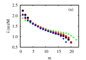
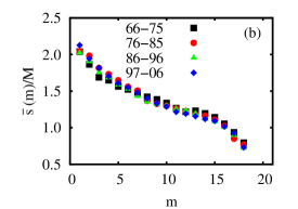
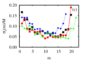
Figure 1: (a) $\bar{s}(m)$ and (c) $\sigma_{s}(m)$ for German Bundesliga (diamonds), English League (squares), Spanish League A (circles) and Spanish League A (triangles). (b) $\bar{s}(m)$ for several periods of German Bundesliga.

As database we have taken the results from the German BundesligaFedAlema in the period from 1965 to 2007 (41 seasons, except the season 1991/92 because it contained more than 18 teams), from the English LeagueFedIngles (12 seasons, 1995-2007), from the Spanish League AFedEspanha (11 seasons, 1996-2007) and from the Spanish League BFedEspanha (9 seasons, 1998-2007).

In every tournament every team plays against all the others twice in each season, once at home and once away, totaling $M$ matches. The standard score system used in many sports leagues, especially in soccer tournaments, states 3 points for a win, one point for a draw and no points for a defeat. However, the score system we found was different: in the past it stated 2 points for a win, rather than 3. The year when the “3 points for a win” was adopted is different for each league. In our data set, only the results from the German Bundesliga mix the two score systems. This league adopted the current system in 1995, the year when FIFA (Fédération Internationale de Football Association) formally adopted the new system, which became standard in international tournaments, as well as most national soccer leagues. Hence, to ensure that our data have a unique score system, we recalculate the scores from German Bundesliga using the actual scheme.

We will represent the score of the rank $m$ in the season $i$ in the round number $r$ as $s_{i}(m,r)$. This quantity is like a microscopic measurement, and therefore is subject to fluctuations. In order to minimize the fluctuations, we start investigating the average of this quantity over the seasons in the final round $r_{f}$, i.e.,

$$\bar{s}(m)=\frac{1}{N}\sum_{i=1}^{N}s_{i}(m,r_{f}),$$ (1)

where $N$ is the number of seasons. Figure 1a shows $\bar{s}(m)$ for all the empirical data set. We can see that $\bar{s}(m)$ presents a similar shape for all leagues, even though the number of teams is different. Someone could argue about a possible time-dependent behavior of this shape. In order to verify it we calculated $\bar{s}(m)$ over four distinct periods of Germany Bundesliga and, as shown in Figure 1b, the shape does not change significantly.

Next, we investigate the standard-deviation of the variable $s_{i}(m,r_{f})$ as a rank function:

$$\sigma^{2}_{s}(m)=\frac{1}{N-1}\sum_{i=1}^{N}[s_{i}(m,r_{f})-\bar{s}(m)]^{2}.$$ (2)

Figure 1c shows this quantity for all empirical data. Again, we found a similar shape for all leagues. Note that these fluctuations are larger for both extremal ranks. A similar result has been recently reported for the average win fraction of baseballSire .

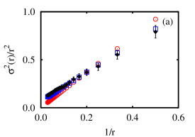
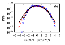
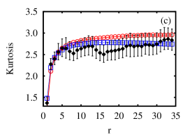
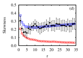
Figure 2: Statistical analysis of Germany Bundesliga; observational data (diamonds), minimalist model (circles) and non-identical team model (squares). (a) Variance $\sigma^{2}(r)$. (b) Probability distribution of scores (PDF) compared with a Gaussian (continuous line). The coefficient of (c) kurtosis and (d) skewness versus $r$. The error bars are calculated via bootstrap resampling method Efron .

This analysis can be extended to a microscopic point of view if we consider the soccer or any other leagues as set of erratic trajectories. A possible manner to establish this correspondence is supposing that the teams are like particles and the scores are the positions. The “motion” is governed by the match result. At each round (time) a team (particle) can jump three units of length to the right (if the team wins) or one unit of length to the right (if the team draws) or stay in the same position (if the team loses). We have, therefore, a random walk-like process: for each team, at the first round, there are only 3 allowed “positions” ($0,1,3$), at the second round there are 6 ($0,1,2,3,4,6$), and so on.

This type of analysis needs a larger number of data. Thus, we will use the results from Germany Bundesliga, because it has more data. We start investigating the standard-deviation over all seasons as a function of the round number $r$, given by

$$\sigma^{2}(r)=\frac{1}{NT-1}\sum_{i=1}^{N}\sum_{m=1}^{T}(s_{i}(m,r)-\mu(r))^{2}\,,$$ (3)

where

$$\mu(r)=\frac{1}{NT}\sum_{i=1}^{N}\sum_{m=1}^{T}s_{i}(m,r)$$

and $T$ is the number of teams. Figure 2a shows $\sigma^{2}/r^{2}$ versus $1/r$. In this representation, the diffusive process can be interpreted as usual random walk with a drift, i.e.,

$$\frac{\sigma^{2}(r)}{r^{2}}=a+\frac{b}{r}$$ (4)

where $a$ and $b$ are essentially variances related with the teams’ fitness and statistical fluctuationsHeuer . Here we have $a\approx 0.075$ and $b\approx 1.55$.

We also evaluate the probability distribution function (PDF) of the scores (for the collapsed data, i.e., all seasons of the Germany Bundesliga with all rounds together) and compare it with a Gaussian distribution as shown in Figure 2b. This result indicates that the scores are not normally distributed, having a short and asymmetric tail extending towards more positive values. This feature becomes more evident when we look for the kurtosis (Figure 2c) and skewness (Figure 2d) coefficientsStatistics . The asymmetric tail reflects the asymmetry in the score system, i.e., the 3 points for a win. We will see that (from our simulations results) if the winner sums 2 points rather than 3 the skewness tends to zero.

3 Modelling

In the previous session, we presented some observational features of the soccer leagues. Now, we will firstly present a minimalist model and subsequently another one which reproduces these observational behaviors very well.

3.1 A minimalist model

As a first attempt to model the previous results, we can use a mean-field-like approximation. In this approach, we consider that all teams are identical and that the match results are obtained from a simulation algorithm. The procedure to simulate a match between two teams $i$ and $j$ starts drawing two uniform random numbers, $x_{i}$ and $x_{j}$, in the interval [0,1]. Thus, we use them in the following algorithm:

IF $$|x_{i}-x_{j}|\leq\delta x_{i}>x_{j} i j$$        the game ends in a draw; ELSE        IF             the winner is the team ;        ELSE             the winner is the team ; (12)

of which the outcome of the game emerges. If we were considered other tournaments (for instance, basketball) where there are no draws, the first step of this algorithm would have to be eliminated.

Employing this procedure, we simulated an entire season $10^{5}$ times. This minimalist model has only one parameter $\delta$ associated with the draws. We incrementally update the values of $\delta$ to minimize, via the method of least squares, the difference between the simulated values of $\bar{s}(m)$ and the observational ones. The best values for this parameter are close together: $\delta=0.11$ for German Bundesliga and the Spanish League A; $\delta=0.15$ for the Spanish League B and $\delta=0.10$ for the English League.

A comparison between simulated and observational data is shown in Figure 3 and, as we can see, this minimalist model can not explain the behavior of $\bar{s}(m)$ found in the empirical data. The discrepancy between model and simulation is larger in the English League and smaller in the Spanish League B. We will see that these discrepancies are related with the difference between the teams, which are greater in the English League than in the Spanish League B. We also evaluate $\sigma^{2}_{s}(m)$ from this model and, as shown in Figure 4, it only describes the data behaviour qualitatively.

For completeness, we also evaluate the standard-deviation $\sigma(r)$, the PDF and the coefficients of kurtosis and skewness shown in Figure 2. Since this model is a mean-field-like approximation, we do not expect it to reproduce the non-Gaussian behavior present in the data. In fact, for this case, the central limit theorem states that the PDF of the sum of many independent random variables tends to a normal distribution. This fact becomes evident if we note that kurtosis and the skewness tend to the normal values (see Figures 2c and 2d).

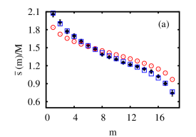
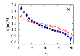
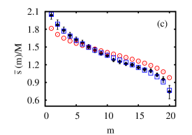
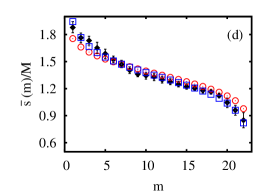
Figure 3: Average rank score: a comparison between observational data (diamonds), minimalist model (circles) and non-identical team model (squares) for (a) German Bundesliga, (b) English League, (c) Spanish League A and (d) Spanish League B.

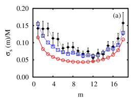
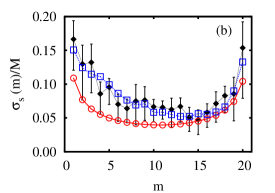
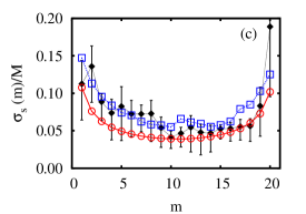
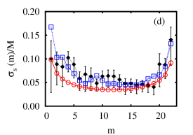
Figure 4: Standard-deviation of the rank scores: a comparison between observational data (diamonds), minimalist model (circles) and non-identical team model (squares) for (a) German Bundesliga, (b) English League, (c) Spanish League A and (d) Spanish League B.

3.2 A non-identical team model

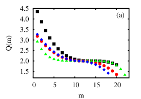
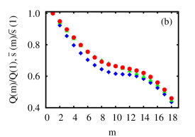
Figure 5: (a) The quality factors $Q(m)$ that emerge from non-identical team model for German Bundesliga (diamonds), English League (squares), Spanish League A (circles) and Spanish League B (triangles). (b) A comparative presentation of $Q(m)$ (diamonds) and rank average for 10 rounds (triangles) and 100 rounds (circles).

Now, we need some additional ingredients to describe the discrepancies previously indicated. Evidently, in a soccer match, the final result is governed by many unforeseen effects which are generally very difficult to model. Thus, we effectively focus our attention on the difference between the teams. It is common sense that the teams are non-identical; for example, they have different offensive and defensive strengths. But how to model these differences? For instance, one soccer report could suggest that the teams are divided into two groups: the small and the big teams.

In this work, as a first approximation, we suppose that each team is fully characterized by only one parameter $Q$, i.e., a single quality factor. Recently, by considering the Bundesliga, a careful investigation pointed that the quality of a team is better described by goal difference than the number of points and that it is constant over each seasonHeuer . However, due to minimalist approach desired in this work, our model does not take some particular ingredients into account, such as, temporal variations over the seasons, home advantage, team-specific characterization, and specific details about the quality factor (e.g., goals difference instead of number of points). Moreover, we emphasize that $Q$ refers to an average behavior of several championships, therefore $Q$ is not related with a specific team nor with its rank within a particular tournament.

It is desirable to employ a functional form of $Q$ with few parameters in contrast with the many parameters (the number of teams) necessary to fully specify $Q$. In this direction, we note that our data (see Figures 1a and 1c) remember the shape of $f(x)\sim-|x|^{\alpha}$ shifted. Thus, in order to take these aspects into account and to overcome possible divergences, our guess is to assume that $Q$ versus rank ($m$) has the very adjustable functional form

$$Q(m) = 2+\frac{T-2m-\epsilon-\beta/2}{T}$$ (13)

$$\times \left|\left({\frac{T-2m-\epsilon-\beta/2}{T}}\right)^{\alpha-1}\right|\,,$$

where $\epsilon$ is a very small number ($\epsilon\ll 1$), $\alpha\geq 0$ and $\beta$ are parameters that dictate the $Q(m)$ form. When $\alpha$ is zero the teams are distributed into two groups ($Q_{1}=1$ and $Q_{2}=3$). The increasing of $\alpha$ begins to distinguish the teams in a continuum. The curve translates to the right if $\beta<0$ or to the left if $\beta>0$ and, when $\beta=0$, the function $Q(m)-2$ is odd with respect to $m=T/2$.

In the direction of a simple model, we would like to emphasize that the choice of $Q(m)$ via eq. (13) is an attempt, motivated by the data, to promote a good adjustment of the model by using a minimal number of parameters. Of course, other forms for $Q(m)$ may be employed, for instance, we could also consider it based on a normal distribution, log-normal distributionJames or linear combination of two normal distributionsHeuer . When considering our data, these possibilities do not give a significant improvement in the results.

In order to use this quality factor, we make a change in the previous simulation algorithm (12). The two random numbers $x_{i}$ and $x_{j}$ are now respectively distributed in the interval $[0,Q(i)]$ and $[0,Q(j)]$, where $Q(i)$ is the quality factor of the team $i$ and $Q(j)$ is the same for the team $j$, in addition, to relativize the parameter $\delta$ we replaced it for $\delta^{\prime}=\delta\frac{Q(i)}{Q(j)}$ with $i>j$. Thus, we are working with the constrained random walk

$$s(i,r+1)=s(i,r)+\xi_{i}\,,$$ (14)

where $\xi_{i}=3$ (1 or 0) if the team $i$ wins (draws or defeats) at $(r+1)$th round and for the team $j$ we have $\xi_{j}=0$ (1 or 3) due to the constraint.

We performed the simulation varying the model parameters ($\alpha$, $\beta$ and $\delta$) to minimize, via the method of least squares, the difference between the simulated values of $\bar{s}(m)$ and the data set ones. The best values for the parameters are shown in Table 1. Note that, besides the changes of statistical properties of German Bundesliga during more than 40 years, the parameters $\alpha$ and $\delta$ corresponding to the last decade (1997-2007) are similar. This model not only reproduces $\bar{s}(m)$ very well (see Figure 3), but it also correctly describes the behavior of the standard-deviation $\sigma^{2}_{s}$ (see Figure 4).

Table 1: The best values for the parameters.

League	Period	$\alpha$	$\beta$	$\delta$
German Bundesliga	1965-2007	2,10	-8,29	0,40
German Bundesliga	1997-2007	2,08	-12,00	0,42
English League	1995-2007	2,99	-17,29	0,45
Spanish League A	1996-2007	2,33	-6,94	0,41
Spanish League B	1998-2007	5,18	-3,30	0,40

Further aspects of the random walk-like process described in Section 2 are in very good agreement with the present model. In fact, as shown in Figure 2, the present model explains the behavior of the variance $\sigma^{2}(r)$, kurtosis, skewness and the PDF.

From our fit, we have obtained the functional form of $Q(m)$ shown in Figure 5a. This function gives us some information about the championship competitiveness. In the previous section, we saw that the minimalist model gives a better agreement for the Spanish League B data. Now, we can note that the shape of $Q(m)$ for this case has more teams in the same baseline than all others. This result indicates that the Spanish League B is the most balanced league from all the empirical data set. On the other hand, the English League presents the most different shape. Note that the quality factors of the first ranks are substantially greater than the others. Therefore, the minimalist model gives poor agreement for this league. This result suggests that in this league there are some teams which are very strong. In fact, from 1995 to 2007, only three teams won this championship, unlike there are eleven different champions in the same period of the Spanish League B.

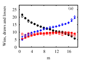
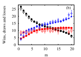
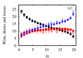
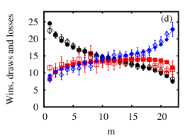
Figure 6: Number of wins (circles), draws (squares) and losses (diamonds) versus rank from observational data (not filled markers) and non-identical team model (filled markers) for (a) German Bundesliga, (b) English League, (c) Spanish League A and (d) Spanish League B.

Finally, we remark some aspects about the quality factor $Q(m)$ and mean number of points $\bar{s}(m)$. Note that $\bar{s}(m)$ is the mean obtained from a very large number of tournaments, which does not coincide with the mean of a tournament with a very large number of rounds. For instance, in a hypothetical tournament with two (identical or not) teams playing only one game without draw we always have $\bar{s}(1)=3$ and $\bar{s}(2)=0$; in contrast, we obtain $\bar{s}(1)=1.5$ and $\bar{s}(2)=1.5$ when the number of matches goes to infinity for identical teamsRibeiro .

Notice also that the result of a match depends on the quality of the involved teams, thus each $\bar{s}(m)$ would be function of all quality factors. Therefore, each $Q(m)$ is a function of all $\bar{s}(m)$. Unfortunately, is not an easy task to obtain a close form of $Q(m)$ in terms of $\bar{s}(m)$ due the non-linearity of the system of equations to be inverted. However, their shapes are in general similar, for example, Figure 5b shows this fact for the German Bunsdesliga when $r\rightarrow\infty$. We also do not have a direct expression for the parameters $a$ and $b$ in eq. (4) in terms of $Q(m)$.

4 Number of wins, draws and losses.

Until now, we have analyzed only the teams’ scores. Another perspective is to analyze the number of wins, draws and defeats. In order to do this, we evaluate the mean value of these quantities over all the empirical data set and the emerging results from the non-identical team model. These results were obtained through simulations of an entire season using the best fit parameters (Table 1). In each simulation we counted (at the final round) the number of wins, draws and defeats of the rank $m$ and them we took an average over $10^{5}$ simulated seasons. A comparison between these two data can be found in Figure 6. Although the model is based on the scores, it gives a good agreement with the observational data. However, we observe that these variables fluctuate more than the scores. This behavior is plausible, since the scores are constructed as a linear combination of this three variables.

We can see that the numbers of wins and defeats have a well defined hierarchical form. For instance, in the case of the number of wins, it is greater for the first ranks and small for the last ones. However, this hierarchical form is not clear when we look at the number of draws. The data behavior suggested that the number of draws is almost constant over the rank positions.

5 Comparison between tournament systems: an application

When dealing with sports tournaments, one can ask about what kind of tournament system is better: the all-play-all or the elimination tournaments? Here, we make an application of our model and compare these tournament systems from a quantitative point of view.

In this context, we take the 16 best teams’ quality factors which emerge from model after the adjustment. Then, we use them to simulate an entire season $10^{5}$ times from both tournament systems. Here, an entire season of the elimination tournaments consists of 4 rounds: the eight-finals, quarter-finals, semi-finals and the final. In this kind of tournaments the loser of each match is immediately eliminated from the championship, for this reason, it is also referred to as “sudden death” tournament.

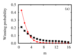
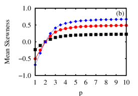
Figure 7: (a) Winning probability of a team with quality factor $Q(m)$ in an all-play-all (diamonds) tournament and in an elimination (squares) tournament. We used the model parameters that emerge from the German Bundesliga data. (b) Mean skewness versus number of points for a win, $p$, for $\delta=0.2$ (squares), $\delta=0.4$ (circles) and $\delta=0.4$ (diamonds).

Employing this procedure and counting how many times a given team won the championship, we get the probability of winning $P(Q(m))$ in the two tournament systems. Figure 7a shows this probability as a function of the rank position by considering the German Bungesliga. Note that the teams with great quality factors are considerably more likely to win in an all-play-all system than in an elimination one. On the other hand, teams with small quality factor are more likely to win in an elimination tournament. This result indicates that an elimination tournament has more randomness which enables less prepared teams to win. Unlike it, the all-play-all system has more games and the randomness decreases which makes it less likely for a team with small quality factor to win.

We also investigated the asymmetric tail characterized by positive skewness. More specifically, we evaluated the mean value of the skewness over $10^{5}$ simulated seasons for several numbers of points for a win, $p$ (as already pointed, $p=3$ corresponds to the current system). In this simulation we use the identical team approach and some values of $\delta$, as shown in Figure 7b. These results indicate that the asymmetric tail is caused by the different score intervals between all possible results. In the most symmetric way, i.e., no points for a defeat, $1$ point for a draw and $2$ for a win, the skewness is approximately $0$ for all values of $\delta$. As $p$ increases, skewness also increases. However, for large values of $p$ the mean skewness is approximately constant. When $p$ is large compared with $1$ (point for a draw), it dominates the score results and consequently the mean skewness saturates. We can note that this plateau depends on the values of the parameter $\delta$, i.e., the plateau is larger for larger values of $\delta$.

6 Summary

In this work we investigated statistical aspects of soccer tournaments. The dynamics of these competitive systems was simulated by a simple probabilistic model, which retains relevant aspects of the leagues, such as the average rank score and the standard-deviations. Our results were compared with data from the German, the English and the Spanish soccer leagues and showed to be in good agreement with them. Also, from these known data, the time evolution of the scores was studied as a random walk-like process. These results indicated that the scores are not normally distributed, due to the difference between the teams and the asymmetry of the scores system. In addition, by using our model, we compared two tournament systems: the all-play-all and the elimination tournaments. This comparison indicated that the eliminatory systems have more randomness, which enables less prepared teams to win the tournament. In the all-play-all systems, the randomness is smaller making the victory of the best teams more likely. In a more general context, due to a high degree of agreement between empirical data and the model, we expect that the random walk-like model employed here may be useful to discuss other kind of tournaments.

- (1) S.Y. Auyang, Foundations of Complex-Systems (Cambridge University Press, Cambridge, 1998).
- (2) H.J. Jensen, Self-Organized Criticality (Cambridge University Press, Cambridge, 1998).
- (3) R. Albert, A.-L. Barabási, Rev. Mod. Phys. 74, 47 (2002).
- (4) H. Haken, Information and Self-Organization (Springer, Berlin, 2006).
- (5) N. Vandewalle, M. Ausloos, P. Boveroux, A. Minguet, Eur. Phys. J. B 4, 139 (1998).
- (6) C.K. Peng, S.V. Buldyrev, A.L. Goldberger, S. Havlin, F. Sciortino, M. Simons, H.E. Stanley, Nature 356, 168 (1992).
- (7) S. Picoli, R.S. Mendes, Phys. Rev. E 77, 036105 (2008).
- (8) S. Chandrasekhar, Rev. Mod. Phys. 15, 1 (1943).
- (9) H.C. Berg, Random Walks in Biology (Princetom University Press, Princetom, 1993).
- (10) R.N. Mantegna, H.E. Stanley, An Introduction to Econophysics (Cambridge University Press, Cambridge, 1999).
- (11) N. Hirotsu, M. Wright, The Statistician 52, 591 (2003).
- (12) M.E. Glickman, H.S. Stern, J. Am. Stat. Ass. 93, 441 (1998).
- (13) R.H. Koning, M. Koolhaas, G. Renes, G. Ridder, Eur. J. Oper. Res. 148, 268 (2003).
- (14) J. Goddard, I. Asimakopoulos, J. Forecast 23, 51 (2004).
- (15) D. Dyte, S.R. Clarke, J. Op. Res. Soc. 51, 993 (2000).
- (16) L.C. Malacarne, R.S. Mendes, Physica A 286, 391 (2000).
- (17) J. Greenhough, P.C. Birch, S.C Chapman, G. Rowlands, Physica A 316, 615 (2001).
- (18) E. Bittner, A. Nußbaumer, W. Janke, M. Weigel, Europhys. Lett. 78, 58002 (2007).
- (19) E. Bittner, A. Nußbaumer, W. Janke, M. Weigel, Eur. Phys. J. B 67, 459 (2009).
- (20) S.R. Clarke, J.M. Norman, The Statistician 44, 509 (1995).
- (21) S. Dobson, J. Goddard, Eur. J. Oper. Res. 148, 247 (2003).
- (22) R.S. Mendes, L.C. Malacarne, C. Anteneodo, Eur. Phys. J. B 57, 357 (2007).
- (23) R.N. Onody, P.A. de Castro, Phys. Rev. E 70, 037103 (2004).
- (24) A. Heuer, O. Rubner, Eur. Phys. J. B 67, 445 (2009).
- (25) H. V. Ribeiro, Undergraduate Monograph, Universidade Estadual de Maringá, (2008).
- (26) http://www.dfb.de/
- (27) http://www.premierleague.com/
- (28) http://www.lfp.es/
- (29) C. Sire, S. Redner, Eur. Phys. J. B 67, 473 (2009).
- (30) B. Efron, R. Tibshirani, An Introduction to the Bootstrap (Chapman & Hall, 1993).
- (31) R.V. Hogg, A. Craig, 5th edn. Introduction to Mathematical Statistics (Prentice Hall, New York, 1995).
- (32) B. James, J. Albert, H.S. Stern, Chance 6, 17 (1993).