Earthquake Forecast via Neutrino Tomography

Abstract

We discuss the possibility of forecasting earthquakes by means of (anti)neutrino tomography. Antineutrinos emitted from reactors are used as a probe. As the antineutrinos traverse through a region prone to earthquakes, observable variations in the matter effect on the antineutrino oscillation would provide a tomography of the vicinity of the region. In this preliminary work, we adopt a simplified model for the geometrical profile and matter density in a fault zone. We calculate the survival probability of electron antineutrinos for cases without and with an anomalous accumulation of electrons which can be considered as a clear signal of the coming earthquake, at the geological region with a fault zone, and find that the variation may reach as much as 3% for $\bar{\nu}_{e}$ emitted from a reactor. The case for a $\nu_{e}$ beam from a neutrino factory is also investigated, and it is noted that, because of the typically high energy associated with such neutrinos, the oscillation length is too large and the resultant variation is not practically observable. Our conclusion is that with the present reactor facilities and detection techniques, it is still a difficult task to make an earthquake forecast using such a scheme, though it seems to be possible from a theoretical point of view while ignoring some uncertainties. However, with the development of the geology, especially the knowledge about the fault zone, and with the improvement of the detection techniques, etc., there is hope that a medium-term earthquake forecast would be feasible.

Introduction.—Earthquakes and tsunamis are natural catastrophes. They occur on our globe so frequently and cost thousands of lives and immense loss of property. We lack an efficient way to forecast earthquakes at present. We believe that our knowledge of modern physics and sophisticated detection techniques and facilities may help. It has been proposed that we could explore oil storage with neutrino beams oil-Glashow ; oil-Smirnov ; oil-Winter , which also find applications in various other fields B-L.Young ; various-applications . These creative ideas motivate us to investigate the possibility of forecasting earthquakes and tsunamis in terms of matter effects on (anti)neutrino oscillations.

Various neutrino experiments are, or will soon be, in operation. With great effort, most neutrino parameters have been determined with certain accuracy. However, the complex phase $\delta_{\rm CP}$ and the sign of $\Delta{m}^{2}_{31}$ are still unknown. Moreover, so far we only have the upper bound of $\theta_{13}$, which is manifestly smaller compared with the other two mixing angles. Precise measurement of $\theta_{13}$ will be valuable for searches for CP violation in the lepton sector. Two reactor neutrino experiments, Daya Bay Daya-Bay in China and Double Chooz Double-Chooz in France, aiming to measure $\theta_{13}$ are expected to reach very high precision at the percent level.

Matter effects on the neutrino oscillation are crucial in some cases, for example, to explain the solar neutrino flux deficit. Wolfenstein Wolfenstein formulated the matter effect on neutrino oscillation and then Mikheev and Smirnov MS applied and developed the theory to successfully solve the solar neutrino problem. The newest experimental data confirm the MSW model.

As a neutrino traverses through matter, its oscillation length is no longer the same as in vacuum. Electron neutrinos acquire an extra potential $V(x)=\sqrt{2}G_{F}n_{e}(x)$ in the Hamiltonian due to their interaction with electrons, which exist in ordinary matter, where $G_{F}$ is the Fermi coupling constant and $n_{e}$ is the number density of electrons in matter. In a simplified version with only two generations, the expression of the survival probability in uniform matter is similar to the vacuum case, but the vacuum mixing angle $\theta_{0}$ and mass-squared difference $\Delta m^{2}=|m_{2}^{2}-m_{1}^{2}|$ should be replaced by the corresponding quantities in matter. That is

$$\ P_{\nu_{e}\rightarrow\nu_{e}}=1-\sin^{2}{2\theta_{M}}\sin^{2}\left({\Delta m_{M}^{2}\over 4E_{\nu}}L\right),$$ (1)

where $\theta_{M}$ and $\Delta m^{2}_{M}$ are the mixing angle and mass-squared difference in matter, respectively. $E_{\nu}$ and $L$ are, respectively, the energy of the neutrino and the length of the baseline. For $\theta_{M}$ we have

$$\tan{2\theta_{M}}=\tan{2\theta_{0}}\left({1-{2\sqrt{2}E_{\nu}G_{F}n_{e}\over\Delta m^{2}\cos 2\theta_{0}}}\right)^{-1}.$$ (2)

For antineutrinos, the minus sign in Eq. (2) should be replaced by a plus sign, which implies that unlike the case of neutrino oscillation in the sun, no resonant stage exists, but an enhancement of the survival probability for antineutrinos, as discussed in neutri-phys .

In analogy to the X-ray tomography, the possibility that (anti)neutrinos could be treated as a probe to detect the inner structure of the earth has been discussed by several authors. Two approaches tomography have been suggested for different (anti)neutrino energies.

Our simplified model for an earthquake fault zone.—Earthquakes are caused by rapid slippage along faults and release of energy stored in the seismic zone. Generally, a seismic zone does not consist of one single fault. The term ” fault zone” implies that the zone is composed of several inner faults and undergoes tremendous deformation caused by severe shear and strain.

On May 12 of 2008, an $M_{S}$= 8.0 earthquake occurred in Wenchuan, Sichuan Province, China. It was caused by the fracture of faults in the Longmenshan fault zone. This fault zone is composed of three parallel faults. The Wenchuan-Maoxian fault is the west most one. According to geological studies, the Longmenshan fault zone is stressed by the west Bayan Har Block and Sichuan Basin yanxing-li , and a 300 km long and 50 km wide deformation zone was formed horizontally.

The simplified geometric structure of the fault zone, which we are going to use in this work, is a cuboid with length $l$ = 300 km, width $w$ = 50 km and depth $d$ = 10 km, and with an upper edge parallel to the earth’s surface. In general, a crust extends to a depth of 30 km crust-depth , and this cuboid is just located at its middle layer. The main shock of the Wenchuan earthquake has a hypocenter depth of about 14 km, and

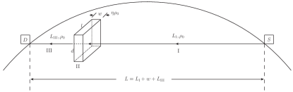
Figure 1: The configuration of the trajectory of the (anti)neutrino beam which is produced in the source $S$, propagates through slabs $\rm{I}$, $\rm{II}$ and $\rm{III}$, and reaches the detector $D$. The baseline length $L$=$L$_I+$w$+$L$_III. The geometry of the fault zone is described by three parameters, length $l$, depth $d$ and width $w$. The matter density of each slab is also marked in the figure.

this hypocenter is inside the cuboid. A schematic of the cuboid is shown in Fig. 1.

The geological structure with a fault zone is not stable and sometimes varies actively. The drastic variations within the region of such geological structure can induce severe earthquakes. Before an earthquake takes place, the variation in the matter density, or more exactly, the electron density of the fault zone is the most significant factor. The relevant effects are categorized into four aspects:

• Strain. Strain can change the matter density directly. During the Wenchuan earthquake, the Longmenshan fault zone is strained by the west and east geological blocks. The map of strain intensity drawn by a professional research group zuan-chen shows that the eastern edge of the Qinghai-Xizang Plateau is close to the region where strain intensity changes steeply. The Longmenshan fault zone undergoes the steepest change. The strain intensity on the west side is four times larger than that on the east side.

• Shear. Shear plays an important role in the slippage of the fault. It can either increase or decrease the matter density. From the maximum shear strain rate map of the Bayan Har Block and Sichuan Basin yanxing-li , one can observe that the maximum shear strain rate of the east of the Longmenshan fault zone is 5$\times 10^{-9}/a$, whereas on the west side, Bayan Har Block, it is 15 $\sim$ 50$\times 10^{-9}/a$. The picture indicates that the shear contrast of both sides is 3 $\sim$ 10.

• Anomalous electric field. The total electron content (TEC) anomaly, as one of the precursors of an earthquake, has been observed from the TEC map using the GPS satellites. The authors of Ref. TEC30-90 point out that, for strong mid-latitudinal earthquakes, the seismo-ionospheric anomalies are manifested as a local TEC increase or decrease in the vicinity of the forthcoming earthquake epicenter, and this phenomenon appears several days prior to the main shock and the TEC modification can be as large as 30 $\sim$ 90 % of the normal value. The physical mechanism for such ionospheric anomalies is that an anomalous electric field is produced near the epicenter. Prior to an earthquake, intensive gas discharges occurring at the crust in the earthquake preparation zone lead to an anomalously strong vertical electric field TAO . The TEC disturbances are the vertical drift of the ionospheric plasma under the influence of the anomalous electric field. On the other hand, if the anomalous vertical electric field definitely exerts influence on the earthquake preparation zone, it can also change the distribution of free electrons in the fault zone. In particular, the research into conductivity characteristics indicates that a low resistance thrust fault zone in the middle layer of the Longmenshan fault zone was observed low-resistance .

• Rock dehydration. Under the influence of tremendous strain and shear, rock would undergo a dehydration process, which also contributes to the density shift in the fault zone dehydration .

The first two aspects concern the geometrical deformation, which contributes an accumulation of mechanical energy. When the shear exceeded the friction strength, the faults in the fault zone were unlocked and slipped suddenly shoubiao-zhu .

Density shift and estimation of fault zone width.— As antineutrinos travel inside the medium, the matter potential $V(x)$ is linearly proportional to the electron density. For the medium in the crust, it is reasonable to assume that $N_{e}$ $\approx$ $N_{p}$ $\approx$ $N_{n}$, i.e. the electron fraction number $Y_{e}$ = $N_{e}/(N_{p}+N_{n})$ $\approx$ 0.5, where $N_{e}$, $N_{p}$ and $N_{n}$ correspond to electron, proton and neutron numbers in the crust layer, and write the electron density in the normal crust matter as

$$n_{e}^{0}(x)={\rho_{0}(x)\over 2m_{N}},$$ (3)

where $\rho_{0}$ is the matter density of the normal medium and $m_{N}$ is the mass of nucleon. As discussed above, the electron density is shifted in the fault zone as

$$n_{e}^{f}=\eta n_{e}^{0}.$$ (4)

As pre-earthquake activities in the fault zone are taken into account, $\rho$ varies from $\rho_{0}$ into an effective matter density $\rho_{f}^{\prime}$

$$\rho_{f}^{\prime}=\eta\rho_{0},$$ (5)

which means that in the fault zone the effective matter density shortly before an earthquake, $\rho_{f}^{\prime}$, is $\eta$ times larger than the normal matter density $\rho_{0}$. In fact, because the existence of the anomalous electric field does not directly influence the real matter density, but only contributes to the electron density of the fault zone, the real matter density of the fault zone $\rho_{f}$ would be smaller than $\eta\rho_{0}$, i.e.

$$2m_{N}n_{e}^{f}=\rho_{f}^{\prime}=\eta\rho_{0},$$

$$2m_{N}n_{p}^{f}=\rho_{f}<\eta\rho_{0},$$ (6)

where $n_{p}^{f}$ is the number density of protons in the fault zone cuboid. The experimental observation indicates that there is a definite relation between $\rho_{f}^{\prime}$ and $\rho_{f}$, namely as $\rho_{f}^{\prime}$ increases, $\rho_{f}$ increases too. The antineutrino oscillation determines $\rho_{f}^{\prime}$, and with the data on $\rho_{f}^{\prime}$, we would obtain unambiguous information about $\rho_{f}$ which causes an earthquake.

The study of geology focuses on a single fault or single fracture. Instead, we consider a zone that consists of several faults and has a relatively large width. The fault zone is treated as a slab with a uniform effective matter density $\rho_{f}^{\prime}$.

The width $w$ of the fault zone can also be estimated from an empirical formula TAO

$$w=2\times 10^{0.414M_{S}-1.696}\ \rm{km},$$ (7)

where $M_{S}$ is the magnitude of the earthquake. For the Wenchuan earthquake, $M_{S}$ = 8.0, the width $w$ is about 80 km from Eq. (7), which is the fault zone width we use in our numerical computations.

Configuration and result for the reactor antineutrinos.— The Daya Bay reactor located in Shenzhen is an example and we shall use its corresponding data as the inputs of our numerical computations. The fault zone cuboid in Wenchuan is about 1418 km to Daya Bay. As is shown in the configuration figure, the $\bar{\nu}_{e}$ first traverses the normal medium with a matter density $\rho_{0}$ = 2.8 $g/cm^{3}$ and then enters the fault zone, which has a width $w$ = 50 km.

Since fault zones are not accessible for direct observation, all information concerning details of the zones is still coarse and sparse. Obviously, more concrete and precise information is needed very badly to forecast disasters. Along with the geologic study, theoretical work and new ideas are also necessary. Certainly, abundant geological data and development in seismology are helpful for the improvement of our fault zone picture and further research. In this work, we set $\eta=3$ as a simple demonstration of our scheme.

We suppose that the beam would be detected at the Qinghai-Xizang Plateau, which is 200 km away from the fault zone. This description of the total configuration of the trajectory is shown in Fig. 1.

Under the approximation of $\theta_{13}\sim 0$ the vacuum oscillation probability $P_{\bar{\nu}_{e}\rightarrow\bar{\nu}_{e}}$ within the three-generation scenario can be reduced into the two-generation case. When taking the matter effect into account and considering the normal hierarchy $\bigtriangleup m^{2}_{21}\ll\bigtriangleup m^{2}_{31}\simeq\bigtriangleup m^{2}_{32}$, the small mass-squared difference $\bigtriangleup m^{2}_{21}$ dominates the oscillation as the effect induced by the larger mass-squared difference $\bigtriangleup m^{2}_{31}$ is averaged out for the long propagation neutri-phys . Then the evolution equation is

$$i{{d}\over{dx}}(\hat{\psi}_{\alpha 1},\hat{\psi}_{\alpha 2},\hat{\psi}_{\alpha 3})^{T}={{1}\over{2E_{\nu}}}\hat{\mathbb{M}}(\hat{\psi}_{\alpha 1},\hat{\psi}_{\alpha 2},\hat{\psi}_{\alpha 3})^{T},$$ (8)

where $\hat{\psi}_{\alpha k}(\alpha=e,\mu,\tau;k=1,2,3)$ is the $\nu_{\alpha}\rightarrow\nu_{k}$ effective evolution amplitude and $\hat{\mathbb{M}}$ is given as neutri-phys

$$\left(\begin{array}[]{rrr}s^{2}_{12}\triangle m^{2}_{21}+c^{2}_{13}A_{cc}&c_{12}s_{12}\triangle m^{2}_{21}&-c_{13}s_{13}e^{-i\delta}A_{cc}\\ c_{12}s_{12}\triangle m^{2}_{21}&c^{2}_{21}\triangle m^{2}_{21}&0\\ -c_{13}s_{13}e^{i\delta}A_{cc}&0&\triangle m^{2}_{31}+s^{2}_{13}A_{cc}\end{array}\right),$$ (12)

where $s_{ij}\equiv\sin\theta_{ij}$, $c_{ij}\equiv\cos\theta_{ij}$ and $A_{cc}=2E_{\nu}V(x)$.

Under the approximation $\theta_{13}\sim 0$, the amplitude $\hat{\psi}_{\alpha 3}$ is decoupled from the evolution equations for $\hat{\psi}_{\alpha 1}$ and $\hat{\psi}_{\alpha 2}$, and the effective survival probability $P^{(3)}_{\bar{\nu}_{e}\rightarrow\bar{\nu}_{e}}$ within the three-generation scenario just reduces into $P^{(2)}_{\bar{\nu}_{e}\rightarrow\bar{\nu}_{e}}$ which is the expression in the two-generation case as

$$P^{(3)}_{\bar{\nu}_{e}\rightarrow\bar{\nu}_{e}}=(1-\sin^{2}\theta_{13})^{2}P^{(2)}_{\bar{\nu}_{e}\rightarrow\bar{\nu}_{e}}+\sin^{4}\theta_{13}.$$ (13)

It is noted that the mixing angle $\theta_{23}$ does not explicitly show up in the survival probability of $\bar{\nu}_{e}\to\bar{\nu}_{e}$. Since $\sin^{2}\theta_{13}<5\times 10^{-2}$ (99.73% CL) sin-theta13 , with the assumption $\theta_{13}\sim 0$, the two-generation analysis involving two parameters $\bigtriangleup m^{2}_{21}$ and $\theta_{12}$ would be a good approximation for the realistic case. In fact, the mixing between $\nu_{\mu}$ and $\nu_{\tau}$ is sizable Xingzz , therefore for the long-distance propagation, the oscillation between $\nu_{\mu}$ and $\nu_{\tau}$ is almost complete, i.e. $\sin^{2}2\theta_{23}\approx 1$.

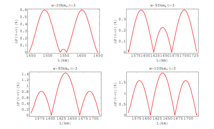
Figure 2: The differences (in percent) in survival probabilities of the reactor electron antineutrino between cases without and with an anomalous accumulation of electrons whose $\eta$ =3 and width $w$ = 20, 50, 80 and 100 km, respectively.

Thus for the practical mixing between $\bar{\nu}_{e}$ and $\bar{\nu}_{x}$, $\bar{\nu}_{x}$ really is the superpositions of $\bar{\nu}_{\mu}$ and $\bar{\nu}_{\tau}$. In the study of the solar neutrino flux missing where only two generations are considered, the updated values of the input parameters are determined as $\sin^{2}2\theta_{0}$ = 0.86 and $\Delta m^{2}$ = 8$\times 10^{-5}$ $\rm{eV}^{2}$. The energy of the reactor electron-antineutrino of $E_{\nu}$ = 3.6 MeV neutri-phys is another input parameter for our numerical computation. The complete formulation involving three generations would make the whole picture very complicated and does not change our qualitative conclusion.

In this configuration, there are three slabs, I, II and III. Each of them is assumed to possess a uniform matter density and can be treated with an $R$-matrix nicolaidis .

$$\left(\begin{array}[]{c}\bar{\nu}_{e}^{\rm{III}}\\ \bar{\nu}_{x}^{\rm{III}}\end{array}\right) = R^{\rm{III}}R^{\rm{II}}R^{\rm{I}}\left(\begin{array}[]{c}\bar{\nu}_{e}^{0}\\ \bar{\nu}_{x}^{0}\end{array}\right).$$ (18)

The elements of the $R$-matrix are determined by the mass-squared difference $\Delta m^{2}_{M}$, neutrino energy $E_{\nu}$ and antineutrino path length in the slab. In a uniform slab, the elements of the $R$-matrices are

$$R_{11} =\exp{\left(i{\Delta m^{2}_{M}\over{2E_{\nu}}}x\right)}+\sin^{2}{\theta_{M}}\left[1-\exp{\left(i{\Delta m^{2}_{M}\over{2E_{\nu}}}x\right)}\right],$$

$$R_{22} =\exp{\left(i{\Delta m^{2}_{M}\over{2E_{\nu}}}x\right)}+\cos^{2}{\theta_{M}}\left[1-\exp{\left(i{\Delta m^{2}_{M}\over{2E_{\nu}}}x\right)}\right],$$

$$R_{12} =R_{21}={1\over 2}\sin^{2}{2\theta_{M}}\left[1-\exp{\left(i{\Delta m_{M}^{2}\over{2E_{\nu}}}x\right)}\right],$$

where $x$ is the antineutrino path length in the slab. we calculate the survival probabilities without

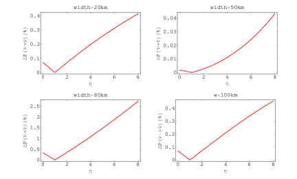
Figure 3: The dependence of the differences (in percent) in survival probabilities between cases without and with an anomalous accumulation of electrons on the $\eta$ value for reactor antineutrinos whose width $w$ = 20, 50, 80 and 100 km, respectively.

and with the anomalous accumulation of electrons at the fault zone. In Fig. 2 we present the differences in survival probabilities of the reactor electron antineutrino between cases without and with an anomalous accumulation of electrons for $\eta$ =3 and different widths. For oscillations in medium with and without the anomalous electron accumulation, the maximal difference in $P_{\bar{\nu}_{e}\rightarrow\bar{\nu}_{e}}$ is up to 2% when the width $w$ = 100 km.

Among all of the fault zone parameters, the width and the $\eta$ value play important roles in antineutrino oscillations. For reactor electron antineutrinos, the dependence of the differences of survival probabilities on $\eta$ is plotted in Fig. 3 with antineutrino energy $E_{\nu}$ = 3.6 MeV for different width values. Fig. 3 indicates that for $\eta<1$, the effect is tiny, and for $\eta$ is larger than one, the predicted probability difference undergoes a relatively larger change with the increase in $\eta$.

Neutrino factory.— Neutrino beams from a neutrino factory neutrino-factory can also be employed in the neutrino oscillation tomography. In our configuration, we choose an electron neutrino beam with energy $E_{\nu}$ = 7 GeV. Our calculation indicates that the difference in survival probabilities corresponding to the cases with and without the anomalous electron accumulation is not obvious. Indeed, an observable difference of about 0.01% may be detected if the detector is 6000 km away from the source. However, such a length of baseline is much beyond the maximal distance in the crust layer and such a small difference may not be detected with the

Parameter	Reactor
Slab	I	II	III
$L$ (km)	1418	$w$	200
$\rho$ $(g/\rm{cm}^{3})$	2.8	$2.8\times 3$	2.8
$\Delta m^{2}_{\rm M}$ $(10^{-5}\rm{eV}^{2})$	$8.02$	$8.09$	$8.02$
$\tan 2\theta_{M}$	2.42	2.30	2.42
$L^{M}_{osc}$ $(\rm{km})$	111.18	110.36	111.18
Parameter	Neutrino Factory
Slab	I	II	III
$L$ (km)	1418	$w$	200
$\rho$ $(g/\rm{cm}^{3})$	2.8	$2.8\times 3$	2.8
$\Delta m^{2}_{\rm M}$ $(10^{-3}\rm{eV}^{2})$	$1.46$	$4.42$	$1.46$
$\tan 2\theta_{M}(10^{-2})$	$-5.10$	$-1.68$	$-5.10$
$L^{M}_{osc}$ $(10^{3}\rm{km})$	$11.92$	$3.92$	$11.92$

Table 1: The parameters of neutrino oscillation in matter for beams produced in a reactor and in a neutrino factory. For reactor electron antineutrinos $E_{\nu}$ = 3.6 MeV and for neutrino factory electron neutrinos $E_{\nu}$ = 7 GeV.

accuracy of the present neutrino facilities in our configuration. The reason is obvious that the accelerator neutrinos have much larger energy than the reactor antineutrinos, thus the oscillation length $L_{osc}^{M}$ for neutrinos from a neutrino factory is much longer than that for the reactor ones as shown in Table 1.

Result from perturbation method.— In a low matter density medium, $V\ll{\Delta m^{2}}/{2E_{\nu}}$, Ioannisian and Smirnov perturbation developed a perturbation method where $\epsilon=2VE_{\nu}/\Delta m^{2}$ is taken as the expansion parameter for calculating the oscillation probability. For the maximal matter density $\eta\rho_{0}$ in our case, one can determine

$$\frac{2E_{\nu}V}{\Delta m^{2}}\approx 0.029\ll 1,$$ (20)

for $E_{\nu}$ = 3.6 MeV and $\eta$ = 3. With the perturbation method, the exact adiabatic phase shift in matter is obtained as

$$\phi^{m}_{a\rightarrow b}=\frac{1}{2E_{\nu}}\int_{a}^{b}dx \biggl{[} \left(\Delta\cos{2\theta_{0}}\pm\sqrt{2}E_{\nu}G_{F}\frac{\rho\left(x\right)}{m_{N}}\right)^{2}$$ (21)

$$+\left(\Delta\sin{2\theta_{0}}\right)^{2}\biggr{]}^{1\over 2}$$

and the plus and minus signs correspond to antineutrinos and neutrinos, respectively. By the formula for flavor-to-flavor transition, we obtain the survival probability of the electron antineutrino originating from the initial spot $x_{0}$ and ending at the final spot

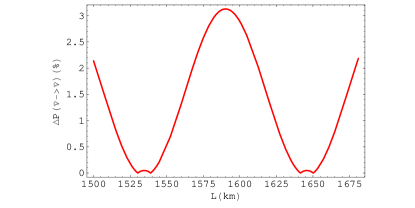
Figure 4: The difference (in percent) of survival probabilities between cases without and with an anomalous accumulation of electrons evaluated in the perturbation theory Eq. (LABEL:P-pertur).

$x_{f}$. Up to the leading order of $V(x)$, we have

$$P_{\bar{\nu}_{e}\rightarrow\bar{\nu}_{e}}= 1 -\sin^{2}{2\theta_{0}}\biggl{[}\sin^{2}{\frac{1}{2}\phi^{m}_{x_{0}\rightarrow x_{f}}}-\frac{\sqrt{2}}{4}\cos{2\theta_{0}}$$

$$\times \int_{x_{0}}^{x_{f}}dx\frac{G_{F}\rho\left(x\right)}{m_{N}}\left(\sin{\phi_{x_{0}\rightarrow x}^{m}+\sin{\phi_{x\rightarrow x_{f}}^{m}}}\right)\biggr{]}.$$

In this scheme, we calculate the survival probability for reactor electron antineutrinos. The result is shown in Fig. 4. The difference in survival probabilities for the cases with and without the anomalous electron accumulation can be as large as 3$\%$, which is larger than the results obtained with the $R$-matrix method.

Discussion.— We note that there is a sharp controversy about the $\eta$ value among geologists. Some think that this value should be rather small, whereas others advocate that, before a severe earthquake, the $\eta$ might reach a sizable value. Taking the advice of the more conservative geologists, we adopt a relatively small value in this work. Indeed, we only investigate the physics and provide a possible way to forecast the earthquake in terms of neutrino medium effects in this work, but we will leave the detailed study of the $\eta$ value to the geologists.

In fact, the other neutrino sources, such as the cosmic muon, would contaminate our detection circumstance. However, we may set some shielding and veto facilities to reduce the uncertainty caused by other neutrino sources. The detailed technical difficulties would be left for our experimental colleagues.

Foreseeing earthquakes in a certain region within ten years, two years and one or two months corresponds to long-, medium- and short-term earthquake forecast, while an impending earthquake forecast should be made a few days before the outbreak. For the long-term and medium-term forecast, there is quite a long duration for the detector to collect sufficient data even though the flux is suppressed by the small solid angle spanned by the detector. For short-term and impending forecasting, the electron density changes drastically as the earthquake is coming, and the overall effect results in a large shift in the oscillation probability in a short time interval, so that observing clear signals might be feasible if the flux from the source is sufficiently strong. As mentioned previously, the geometrical deformation caused by strain and shear would last for a long period, say, hundreds of years in some cases and the deformation would eventually reach its maximum before the outbreak. However, the strong anomalous electric field appears only several days, e.g. about a week before the earthquake, so that the week before the outbreak is crucial for detectors to collect data and reach a conclusion about the upcoming disaster.

Now let us make a rough numerical evaluation of the event rates based on the Daya Bay Monte-Carlo simulation. In the Daya Bay case, the detector is set at 1 km away from the neutrino source, and the detection rate is about a few hundred per day ($\sim$400/day, as estimated). Supposing a shortened baseline in our case is 200km, the suppression factor for the flux would be $1/(200)^{2}\sim 3\times 10^{-5}$. Considering an exposure time of 100 days and assuming that the detection efficiency is 100 times larger than that employed in Daya Bay experiment, the expected events would be at least $\mathcal{O}$(100), which is suitable for a medium-term forecast. For example, in a period of one year, one can compare the events observed in the first half of the year with that in the second half. If these data show an explicit difference in survival probabilities during the two periods, they would imply a geological deformation that may result in an earthquake in the forthcoming period. The closer the earthquake is, the larger the difference.

Indeed, in our present work, we consider idealized beam characteristics while ignoring many details. The uncertainty caused by other neutrino sources such as other reactors and geoneutrinos, is also ignored, which may be one of the main challenges in the implementation of this scheme. Thus we reach our conclusion that with the present reactor facilities and detection techniques, it is still a difficult task to make an earthquake forecast using such a scheme, though it seems to be possible from a theoretical point of view while ignoring some uncertainties. However, there is hope that with the great improvement in detection and innovation of facilities, the sensitivity and efficiency would be greatly improved and the size of the detector may be much larger with sufficient fund support, and with the development of the geology and seismology, the pictures of the fault zone will be clearer and its parameters more accurate, thus a medium-term earthquake forecast would be feasible.

A scheme might remedy the shortcoming of remarkably losing neutrino flux due to the small solid angle. Namely, one may use a low energy beta beam beta-beam as a source. Such a neutrino beam could be directly oriented to the fault zone. Without the $10^{-5}$ suppression factor, the requirement for the size and sensitivity of the detectors would be greatly alleviated. However, in order to obtain intense and collimated neutrino beams from the traditional source for the beta beam, e.g., ${}^{6}_{2}\rm{He}^{++}{\rightarrow}^{6}_{3}\rm{Li}^{+++}+\rm{e}^{-}+\bar{\nu}_{e}$ beta-beam , the high intensity of the ${}^{6}_{2}\rm{He}^{++}$ source and a large Lorentz boost factor are necessary. We suggest alternative schemes. One is that in the process $e^{-}+\rm{p}\rightarrow\rm{n}+\nu_{e}$ we can employ the very collimated electron beam to bombard the protons at rest. Another is that we can use the lowly accelerated pion beam for $\pi^{\pm}\rightarrow e^{\pm}+\bar{\nu}_{e}(\nu_{e})$. Even though in the second proposal, the decay rate is suppressed by the helicity rule, the branching ratio is still of the order of $10^{-4}$ Data , so with a large number of pions, it is still plausible. Moreover, a large Lorentz boost factor $|{\bf p}|/m_{e}$ which determines the spreading solid angle, is easy to obtain and the energy for the pion accelerator needs to be just at $\mathcal{O}(\rm{GeV})$. Thus the size of such facilities can be small and the corresponding technique would be relatively simple.

- (1) Rujula A De, Glashow S L, Wilson R R et al. Phys. Rept., 1983, 99: 341-396
- (2) Ioannisian A N, Smirnov A Y. 2002, arXiv:hep-ph/0201012
- (3) Ohlsson T, Winter W. Europhys. Lett., 2002, 60(1): 34-39
- (4) Young B L, in the proceedings for the conference on the advanced topics in the interdiscipilinary fields of particle physics, nuclear physics and cosmology, Tengchong, China, Aug., 2008
- (5) Wilson T L. Nature, 1984, 309: 38-42; Gonzalez-Garcia M C, Halzen F, Maltoni M et al. Phys. Rev. Lett., 2008, 100: 061802; Akhmedov E K, Tortola M A, Valle J W.F. JHEP, 2005, 0506: 053; Lindner M, Ohlsson T, Tomas R et al. Astropart. Phys., 2003, 19: 755-770; Ohlsson T, Winter W. Phys. Lett., 2001, B512; 357-364; Jain P, Ralston J P, Frichter G M. Astropart. Phys., 1999, 12: 193-198; Sugawara H, Hagura H, Sanami T. 2003, arXiv:hep-ph/0305062
- (6) CAO Jun. Nucl. Phys. Proc. Suppl., 2006, 155: 229-230; CHEN Shao-Min. J. Phys. Conf. Ser., 2008, 120: 052024; White C. J. Phys. Conf. Ser., 2008, 136: 022012
- (7) Dawson J.V. 2009, arXiv:hep-ex/0905.4843
- (8) Wolfenstein L. Phys. Rev. D, 1978, 17: 2369-2374
- (9) Mikheev S P, Smirnov A Y. Sov. J. Nucl. Phys., 1985, 42: 913-917; Nuovo Cim. C, 1986, 9: 17-26
- (10) Giunti C, Kim C W. Fundamentals of Neutrino Physics and Astrophysics. New York: Oxford, 2007
- (11) Winter W. Earth Moon and Planets, 2006, 99: 285-307
- (12) LI Yan-Xing, ZHANG Jing-Hua, ZHOU Wei et al. Chinese J. Geophys., 2009, 52(2): 519-530(in Chinese)
- (13) Stacey F D. Physics of the Earth. New York: John Wiley & Sons, 1977
- (14) CHEN Zu-An, LIN Bang-Hui, BAI Wu-Ming et al. Chinese J. Geophys., 2009, 52(2): 408-417(in Chinese)
- (15) Namgaladze A A, Zolotov O V, Zakharenkova I E et al. Proc. of MSTU, 2009, 12: 308-315
- (16) Pulinets S. TAO, 2004, 15: 413-435
- (17) WANG Xu-Ben, ZHU Ying-Tang, ZHAO Xi-Kui et al. Chinese J. Geophys., 2009, 52(2): 564-571(in Chinese)
- (18) ZHOU Yong-Sheng, HE Chang-Rong. Chinese J. Geophys., 2009, 52(2): 474-484(in Chinese)
- (19) ZHU Shou-Biao, Zhang Pei-Zhen. Chinese J. Geophys., 2009, 52(2): 418-427(in Chinese)
- (20) Fogli G L, Lettera G, Lisi E et al. Phys. Rev. D, 2002, 66: 093008
- (21) XING Zhi-Zhong. Int. J. Mod. Phys. E, 2007, 16:1361-1372
- (22) Nicolaidis A, Jannane M, Tarantola A. J. Geophys. Res., 1991, 96: 21811-21817
- (23) Geer S. Phys. Rev. D, 1998, 57: 6989-6997
- (24) Ioannisian A N, Smirnov A Y. Phys. Rev. Lett., 2004, 93: 241801
- (25) Zucchelli P. Phys. Lett. B, 2002, 532: 166-172
- (26) Particle Data Group. Phys. Lett. B, 2008, 667: 1-1340