Nearest-neighbor coupling asymmetry in the generation of cluster states

Abstract

We demonstrate that charge-qubit cluster state generation by capacitive coupling is anisotropic. Specifically, horizontal vs vertical nearest-neighbor inter-qubit coupling differs in a rectangular lattice. We show how to ameliorate this anisotropy by applying potential biases to the array of double dots.

I Introduction

One-way quantum computing is a particularly attractive model for quantum circuits because global entanglement is accomplished in a single step, and then all subsequent quantum computation is effected simply by sequential feedback-controlled single-qubit measurements RB01 . The globally entangled state that serves as a universal substrate for quantum computation is known as a cluster state and was originally proposed for optical lattices BR01 and subsequently demonstrated with photons WRR+05 . Efficient quantum circuits for one-way quantum computing was proposed for solid state devices TLHN09 .

Solid-state charge-qubit cluster states offer the exciting prospect of one-way quantum computing with semiconductors TLF+06 ; YWTN07 . Here we show that proposals for periodic generation of charge-qubit cluster states involving double-dot (henceforth ‘ddot’ as this term emphasizes the single-entity nature of the ddot structure) charge qubits are complicated by an overlooked inter-qubit coupling asymmetry in two dimensions. We remedy this complication by showing that the original proposals TLF+06 ; YWTN07 can be recovered simply by applying a potential field bias.

We proceed first by establishing the second-quantized Hamiltonian description for the array of quantum dots and then showing how the Hamiltonian can be simplified to a first-quantized Hamiltonian over ddot charge qubits. In the slow tunneling-rate regime, we show that the first-quantized Hamiltonian is well approximated by the ubiquitous Ising-like Hamiltonian. This Hamiltonian considerably simplifies the dynamical description and shows that the necessary bias of the ddot charge qubits to generate cluster states is determined by the number of ddot neighbors. Thus a global bias of a large structure will lead to periodic evolution of excellent approximations to cluster states. Furthermore, by applying different biases only to the ddots on the boundary (and not to the ddots within), the Hamiltonian induces evolution to the ideal cluster state.

Our aim here is to remedy the deficiency of anisotropies in the evolution of ddot charge-qubits. We show that this problem can be nearly remedied by a global field bias and completely remedied by a global field bias with corrective biases applied to the ddots at the boundary. This method for correcting anisotropy is examined numerically for the case of $40$nm GaAs ddots in a two-dimensional lattice formation with $a$ being the distance between two sites of the ddot, $d_{x}$ and $d_{y}$ the distance between both left and right sites of two nearest-neighbor ddots in $x$ direction and $y$ direction in Fig. 1(a), respectively.

II Charge-qubit cluster state

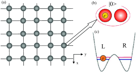
Figure 1: (Color online.) (a) A two-dimensional cluster state. Each grey ball represents a charge qubit, and lines connect nearest neighbors in the horizontal and vertical directions. These lines correspond to coupling by controlled-Z operations. (b) The qubit represented by a grey ball is expanded to a double-dot structure. The logical qubit state $\left|0\right\rangle$ is depicted as the double-dot structure with and extra charge in the left (L) dot. (c) The double-dot structure is modeled as a double-well potential. The blue (lower) pair of lines corresponds to the energy of the symmetric state for the sharing of the excess charge between the two wells, and the red (upper) pair of lines corresponds to the energy of the antisymmetric shared-charge state.

The charge-qubit cluster state (CQCS) in two dimensions is depicted in Fig. 1. The standard depiction of this cluster state is shown in Fig. 1(a) as a periodic rectangular lattice of qubits connected to nearest neighbors by solid lines. Each qubit state is in $\mathcal{H}_{2}={\rm span}\{\left|0\right\rangle,\left|1\right\rangle\}$, with $\left|0\right\rangle$ the logical zero state and $\left|1\right\rangle$ the logical one state. Cluster state generation proceeds first by globally transforming every qubit from the state $\left|0\right\rangle$ to the state $\left|+\right\rangle$ where $\left|\pm\right\rangle:=\left(\left|0\right\rangle\pm\left|1\right\rangle\right)/\sqrt{2}$. We refer to $\{\left|0\right\rangle,\left|1\right\rangle\}$ as the ‘standard basis’ and $\{\left|+\right\rangle,\left|-\right\rangle\}$ as the ‘dual basis’.

After all $N$ qubits in the cluster state are prepared in the $\left|+\right\rangle^{\otimes N}$ state, nearest-neighbor qubits then interact via the two-qubit controlled-$Z$ operations, denoted CZ. Here $Z$ is the Pauli ‘phase’ operator. The other Pauli operators are the ‘flip’ operator $X$, the ‘flip+phase’ operator $Y=XZ$, and the identity operator $\mathds{1}$. This operation is represented in the two-qubit standard basis $\{\left|00\right\rangle,\left|01\right\rangle,\left|10\right\rangle,\left|11\right\rangle\}$ as ${\rm CZ}={\rm diag}\left\{1,1,1,-1\right\}$. The unitary operation CZ is independent of whether the line in Fig. 1(a) is horizontal or vertical.

Fig. 1(b) shows that the horizontal vs vertical symmetry is in fact broken by the coupling axis of the charge qubit, which is represented in Fig. 1(b) as an excess charge in the left or right quantum dot. Although the charge-qubit coupling axis could be aligned independently of the orientation of the overall qubit lattice, we will treat the case that the charge-qubit coupling axis is in the $x$-direction. This is a physically reasonable case, and extending to the case of arbitrary alignment is involved but not difficult.

The charge qubit can be created as a semiconductor ddot structureOo98 . Other alternatives exist such as the superconducting charge qubitDongen94 or a pair of dangling bonds on a surface DB . In any case, the logical states typically correspond either to the left- and right-well occupancy by the excess charge or, alternatively, to the cases of symmetric or antisymmetric charge states between the two dots of a ddot charge qubit.

For coherently evolving charge qubits, Schrödinger’s equation can be used to describe the dynamics, and the potential in Schrödinger’s equation is depicted in Fig. 1(c). Here we treat the standard basis as corresponding to left- and right-occupancy; the dual basis then corresponds to the symmetric and antisymmetric charge-occupancy states.

The quantum dots are engineered so that each potential well has only one bound energy state for the excess electron. Due to the Pauli exclusion principle, the number of electrons in each well is either zero or one or else two electrons with opposite spins. The case of two excess electrons in one double-dot structure should be energetically forbidden by Coulomb repulsion between the two electrons to preserve the integrity of the charge qubit.

III Modeling the dynamics

The goal is to have one excess electron per closely-spaced quantum dot pair, but the general picture is that each quantum dot can have one or two electrons. The restriction of one excess electron must emerge as an energetically favorable configuration rather than be imposed by fiat. The full second-quantized description of the electrons in the array of quantum dots is given by the extended Hubbard model (EHM).

III.1 The extended Hubbard model

The EHM applies to an array of quantum dots whose locations in a two-dimensional array are denoted by lattice coordinates. For $\hat{c}_{ij}$ the annihilation operator at dot site $(i,j)$, $\hat{c}^{\dagger}_{ij}$ the conjugate creation operator, and $\hat{n}_{ij}=\hat{c}^{\dagger}_{ij}\hat{c}_{ij}$ the number operator, the dynamics of the charge-qubit cluster state can conveniently be described by the extended Hubbard Hamiltonian hub (As spin is conserved, we can, without loss of generality, assume fixed spin and ignore this degree of freedom)

$$\hat{H}= \sum_{i,j}E\hat{n}_{ij}+\hat{V}$$ (1)

$$+\sum_{i,j,i^{\prime},j^{\prime}}W_{ij,i^{\prime}j^{\prime}}\hat{n}_{ij}\hat{n}_{i^{\prime}j^{\prime}}-T_{ij,i^{\prime}j^{\prime}}\left(\hat{c}^{\dagger}_{ij}\hat{c}_{i^{\prime}j^{\prime}}+\text{h.c.}\right).$$

Here $E$ is the effective on-site energy for each site $(i,j)$, which can vary due to local field effects. $T_{ij,i^{\prime}j^{\prime}}$ is the coherent tunneling rate between sites $(i,j)$ and $(i^{\prime},j^{\prime})$. $W_{ij,i^{\prime}j^{\prime}}$ is the Coulomb repulsion energy between sites $(i,j)$ and $(i^{\prime},j^{\prime})$. Finally, for $\widehat{\Delta n}_{ij,i^{\prime}j^{\prime}}:=\hat{n}_{ij}-\hat{n}_{i^{\prime}j^{\prime}}$ the number-difference operator between sites $(i,j)$ and $(i^{\prime},j^{\prime})$, the potential bias operator is

$$\hat{V}=\frac{1}{2}\sum_{i,j,i^{\prime},j^{\prime}}V_{ij,i^{\prime}j^{\prime}}\widehat{\Delta n}_{ij,i^{\prime}j^{\prime}}$$ (2)

with $V_{ij,i^{\prime}j^{\prime}}$ the inter-site $(i,j)\leftrightarrow(i^{\prime},j^{\prime})$ potential difference.

In fact Eq. (1) describes not just nearest-neighbor interactions but interactions between all dots with all other dots, where the inter-dot couplings $T_{ij,i^{\prime}j^{\prime}}$ and $W_{ij,i^{\prime}j^{\prime}}$ are suitably chosen. For charge qubits corresponding to closely spaced dot pairs, $T_{ij,i^{\prime}j^{\prime}}$ can be neglected for all but the ddot of a given charge qubit. Also $W_{ij,i^{\prime}j^{\prime}}$ is only significant between charge qubits. The interdot (possibly screened) Coulomb repulsion is neglected for the ddots of a charge qubit because $W_{ij,ij}$ is sufficiently large to prevent both dots from being simultaneously excessively charged.

III.2 Single-qubit gates

Eq. (1) is a second-quantized Hamiltonian. To bridge this Hamiltonian over to the multi-qubit description, we restrict the Hilbert space, upon which the first-quantized version of the Hamiltonian acts, to the case of a single excess electron in each double well. Note here that a dot has lattice coordinates expressed here as $(i_{1},j_{1})$ and dot $2$ is at $(i_{2},j_{2})$.

For an array with close proximity between dots of the ddot pair, the resultant charge-qubit ddot pair can be treated as a point-like object in the quantum computing architecture. This ddot charge qubit has a point-like coordinate designated by  $\mathfrak{(m,n)}$ where the change of font is used to indicate point-like ddot coordinates rather than the coordinates of a particular quantum dot. Thus, we use $(i,j)$ to designate the location of a quantum dot in a two-dimensional array and $\mathfrak{(m,n)}$ to denote the location of a point-like ddot charge qubit.

Assuming two dots of each ddot pair share one electron, the state od ddot pair is a superposition of two basis states: $\{\left|{L}\right\rangle,\left|{R}\right\rangle\}$. Here $L$ ($R$) indicates that the electron is in the left (right) dot. In this basis, $\hat{H}$ in Eq. (1) for one ddot projected onto $\hat{H}_{\mathfrak{mn}}$ is

$$\hat{H}_{\mathfrak{mn}} =E(\left|{L}\right\rangle\left\langle{L}\right|+\left|{R}\right\rangle\left\langle{R}\right|)+V(\left|{L}\right\rangle\left\langle{L}\right|-\left|{R}\right\rangle\left\langle{R}\right|$$

$$+T(\left|{L}\right\rangle\left\langle{R}\right|+\text{h.c.}))=\left(\begin{array}[]{cc}E+V&T\\ T&E-V\\ \end{array}\right)$$ (5)

for $V=V_{L}-V_{R}$ (the relative energy between the left and right dots of a ddot pair), and $T$ is the flip rate corresponding to the tunneling rate between the two dots of a ddot charge qubit.

This Hamiltonian can be conveniently rewritten as a linear combination of three types of quantum gates. These gates are the identity $\openone$, $X=\left|0\right\rangle\left\langle{1}\right|+\left|1\right\rangle\left\langle{0}\right|$, phase gate $Z=\left|0\right\rangle\left\langle{0}\right|-\left|1\right\rangle\left\langle{1}\right|$ with $\left|{0}\right\rangle:=\left|{L}\right\rangle$ and $\left|{1}\right\rangle:=\left|{R}\right\rangle$. With these simplifications, the Hamiltonian (1) can be projected into the qubit space. This projection becomes clear by studying the single-qubit case comprising one ddot pair.

In the standard basis the ddot single-qubit Hamiltonian is $\hat{H}_{\mathfrak{mn}}=E\mathds{1}+TX+VZ$ at site $(\mathfrak{m},\mathfrak{n})$. Here $E$ is an energy term for the qubit. The bias $V$ can be controlled by applying an electric field potential across the ddot pair.

In order to connect our mathematical expressions to a typical experimental setting, we consider a GaAs ddot with a single-dot diameter of $40$nm sci10 . A typical experimental parameter range for tunneling is $T\approx 0-10\mu$eV: here we choose $T=0.1\mu$eV ($160$MHz). By tuning the electric field to $V=0$, the evolution of the Hamiltonian $\hat{H}_{\mathfrak{mn}}$ effectively implements bit flips via the $X$ operator, and the resultant tunneling or flipping rate is $160$MHz. By tuning the electric potential bias to $V\gg T$, e.g. $V=10\mu$eV, the dynamics is dominated by phase flipping at a rate of $16$GHz.

III.3 Two-qubit gates

Now let us consider the two-qubit gate such as the CZ gate, which can be implemented via Coulomb interaction between two nearest-neighbor charge qubits shown below. The Hamiltonian for two nearest-neighbor charge qubits located at $(\mathfrak{m},\mathfrak{n})$ and at $(\mathfrak{m^{\prime}},\mathfrak{n^{\prime}})$ with (possibly screened) Coulomb interaction is

$$\hat{H}_{\mathfrak{mnm^{\prime}n^{\prime}}} =2E\mathds{1}+TX_{\mathfrak{mn}}+V_{\mathfrak{mn}}Z_{\mathfrak{mn}}+TX_{\mathfrak{m^{\prime}n^{\prime}}}$$ (6)

$$+V_{\mathfrak{m^{\prime}n^{\prime}}}Z_{\mathfrak{m^{\prime}n^{\prime}}}+\sum_{l,k=0}^{1}\varsigma_{lk}\left|{lk}\right\rangle_{\mathfrak{mnm^{\prime}n^{\prime}}}\left\langle{lk}\right|.$$

The last term describes the Coulomb interaction energy in the qubit basis between the two nearest-neighbor charge qubits located at $(\mathfrak{m},\mathfrak{n})$ and at $(\mathfrak{m^{\prime}},\mathfrak{n^{\prime}})$ to with sums over $l$ and $k$ representing the two charge qubits are in the state $\left|{l}\right\rangle$ and $\left|{k}\right\rangle$.

The coefficients $\varsigma_{lk}$ are the inter-site Coulomb interaction strengths between the same or opposite sites of the two charge qubits $(\mathfrak{m},\mathfrak{n})$ and $(\mathfrak{m^{\prime}},\mathfrak{n^{\prime}})$. For the case $l=k$, i.e. the two charge qubits are in the same states and both electrons in the left or right dots, we have $\varsigma_{00}=W^{\mathfrak{mnm^{\prime}n^{\prime}}}_{LL}$ and $\varsigma_{11}=W^{\mathfrak{mnm^{\prime}n^{\prime}}}_{RR}$. For the other case $l\neq k$, i.e. the two charge qubits are in different states and the two electrons in different dots, we have $\varsigma_{01}=W^{\mathfrak{mnm^{\prime}n^{\prime}}}_{LR}$ and $\varsigma_{10}=W^{\mathfrak{mnm^{\prime}n^{\prime}}}_{RL}$.

In the 2D lattice shown in Fig. 1(a), for two nearest-neighbor charge qubits there are two cases: both qubits located in the same column (along the $x$ direction) and in the same row (along the $y$ direction). We use the superscripts $x$ and $y$ to distinguish these two cases. For the two nearest-neighbor charge qubits in the same column in which the structure is symmetric, $\varsigma_{00}^{x}=\varsigma_{11}^{x}=V_{\text{Q}}/d_{x}$, and $\varsigma_{01}^{x}=\varsigma_{10}^{x}=V_{\text{Q}}/\sqrt{d_{x}^{2}+a^{2}}$ for $V_{\text{Q}}=e^{2}/(4\pi\epsilon)$ with $\epsilon$ the applicable dielectric constant. In contrast, for the two nearest-neighbor charge qubits in the same row in which the structure is asymmetric, $\varsigma_{00}^{y}=\varsigma_{11}^{y}=V_{\text{Q}}/d_{y}$, $\varsigma_{01}^{y}=V_{\text{Q}}/(d_{y}+a)$, and $\varsigma_{10}^{y}=V_{\text{Q}}/(d_{y}-a)$.

For the GaAs ddot system considered in the previous subsection, we have $V_{\text{Q}}=1.75\times 10^{-29}$N$\cdot$m². With the experimental parameters $a=400$nm, $d_{x}=5.5\mu$m and $d_{y}=5.85\mu$m sci10 , we numerically estimate the coefficients of the interaction terms to obtain $\varsigma_{00}^{x}=\varsigma_{11}^{x}=20.0\mu$eV, $\varsigma_{01}^{x}=\varsigma_{10}^{x}=19.8\mu$eV, $\varsigma_{00}^{y}=\varsigma_{11}^{y}=18.7\mu$eV, $\varsigma_{01}^{y}=17.5\mu$eV and $\varsigma_{10}^{y}=20.1\mu$eV.

IV Generating cluster states

In the one-way quantum computing model, the two-dimensional cluster state is a highly entangled multi-qubit state and processed by performing sequences of adaptive single-qubit measurements, thereby realizing arbitrary quantum computations. The two-dimensional cluster state serves as a universal resource for one-way quantum computing, in the sense that any multi-qubit state can be prepared by performing sequences of local operations on a sufficiently large two-dimensional cluster state NMDB06 .

In previous proposals TLF+06 ; YWTN07 , charge qubits are treated as being symmetrically coupled, which is an appropriate strategy for the one-dimensional case but not at all for the two-dimensional case. Here we show that, by applying local external electric fields, we can generate two-dimensional cluster states without the requirement of symmetry of charge qubits.

In the two-dimensional case shown in Fig. 1(a), we obtain a more general Hamiltonian case with external electric fields $V_{\mathfrak{mn}}$ applied on each qubit $\mathfrak{(m,n)}$ located in the $\mathfrak{m}^{\rm th}$ row and the $\mathfrak{n}^{\rm th}$ column of the ddot charge qubit array:

$$\hat{H}_{\text{2D}}= N^{2}E+\sum_{\mathfrak{m,n}=1}^{N}\Big{[}TX_{\mathfrak{mn}}+V_{\mathfrak{mn}}Z_{\mathfrak{mn}}$$

$$+\frac{1}{2}\varsigma_{+}^{x}\mathds{1}_{\mathfrak{mn}}\otimes\mathds{1}_{\mathfrak{m}+1,\mathfrak{n}}+\frac{1}{2}\varsigma_{-}^{x}Z_{\mathfrak{mn}}\otimes Z_{\mathfrak{m}+1,\mathfrak{n}}$$

$$+\frac{1}{2}(\Delta\varsigma_{+}^{x}+\Delta\varsigma_{-}^{x})Z_{\mathfrak{mn}}+\frac{1}{2}(\Delta\varsigma_{+}^{x}-\Delta\varsigma_{-}^{x})Z_{\mathfrak{m}+1,\mathfrak{n}},$$

$$+\frac{1}{2}\varsigma_{+}^{y}\mathds{1}_{\mathfrak{mn}}\otimes\mathds{1}_{\mathfrak{m,n}+1}+\frac{1}{2}\varsigma_{-}^{y}Z_{\mathfrak{mn}}\otimes Z_{\mathfrak{m,n}+1}$$

$$+\frac{1}{2}(\Delta\varsigma_{+}^{y}+\Delta\varsigma_{-}^{y})Z_{\mathfrak{mn}}$$

$$+\frac{1}{2}(\Delta\varsigma_{+}^{y}-\Delta\varsigma_{-}^{y})Z_{\mathfrak{m,n}+1}\Big{]},$$ (7)

where in order to rewrite the interaction terms in the Pauli operator $Z$, we introduce $2\varsigma_{\pm}^{x(y)}=\varsigma_{00}^{x(y)}+\varsigma_{11}^{x(y)}\pm\varsigma_{01}^{x(y)}+\varsigma_{10}^{x(y)}$, $\Delta\varsigma_{+}^{x(y)}=\varsigma_{00}^{x(y)}-\varsigma_{11}^{x(y)}$, and $\Delta\varsigma_{-}^{x(y)}=\varsigma_{01}^{x(y)}-\varsigma_{10}^{x(y)}$.

For the two nearest-neighbor charge qubits in the same column in which the structure is symmetric, we have $\varsigma_{+}^{x}=V_{\text{Q}}/d_{x}+V_{\text{Q}}/\sqrt{d_{x}^{2}+a^{2}}$, $\varsigma_{-}^{x}=V_{\text{Q}}/d_{x}$ and $\Delta\varsigma_{\pm}^{x}=0$. In contrast, for the two nearest-neighbor charge qubits in the same row in which the structure is asymmetric, we have

$$\varsigma_{\pm}^{y}=\frac{V_{\text{Q}}}{d_{y}}\pm\frac{V_{\text{Q}}}{2(d_{y}+a)}+\frac{V_{\text{Q}}}{2(d_{y}-a)},$$ (8)

$\Delta\varsigma_{+}^{y}=0$, and $\Delta\varsigma_{-}^{y}\equiv\Delta\varsigma=-2V_{\text{Q}}a/(d^{2}_{y}-a^{2})$. By choosing the proper distances $d_{x}$ and $d_{y}$ between the nearest-neighbor charge qubits, we have $\varsigma_{-}^{x}/2=\varsigma_{-}^{y}/2\equiv\varsigma$.

For the GaAs ddot system considered in the previous section, the energy offsets are $\varsigma_{+}^{x}=39.7\mu$eV, $\varsigma_{+}^{y}=37.5\mu$eV, $\Delta\varsigma=-2.6\mu$eV, and $\varsigma=10.0\mu$eV. Note that $\Delta\varsigma$ is comparable to the bias $V_{\mathfrak{mn}}$ hence cannot be neglected.

The Hamiltonian for the two-dimensional array of charge qubits can be simplified as (neglecting identical terms such as $N^{2}E$ and other such terms)

$$\hat{H}^{\prime}_{\text{2D}}= \sum_{\mathfrak{m,n}=1}^{N}\big{[}TX_{\mathfrak{mn}}+V^{\prime}_{\mathfrak{mn}}Z_{\mathfrak{mn}}$$ (9)

$$+\varsigma(Z_{\mathfrak{mn}}\otimes Z_{\mathfrak{m}+1,\mathfrak{n}}+Z_{\mathfrak{mn}}\otimes Z_{\mathfrak{m,n}+1})\big{]},$$

where

$$V^{\prime}_{\mathfrak{mn}}=\left\{\begin{array}[]{ll}V_{\mathfrak{mn}},&\mathfrak{m}=1,\dots,N;\mathfrak{n}=2,\dots,N-1\\ V_{\mathfrak{m}1}-\Delta\varsigma/2,&\mathfrak{m}=1,\dots,N;\mathfrak{n}=1\\ V_{\mathfrak{m}N}+\Delta\varsigma/2,&\mathfrak{m}=1,\dots,N;\mathfrak{n}=N\end{array}\right.$$ (10)

are the modified energy offsets for each ddot pair at site $\mathfrak{(m,n)}$.

For the ddot pairs on the two edge columns, the energy offsets are modified due to the asymmetry of the structure. In contrast, for those in the middle columns, the energy offsets remain and are caused by the applied electric fields because the extra energy offsets are canceled out due to the structure.

V Approximating Ising-like dynamics

We apply a canonical transformation for a global basis change on the Hamiltonian shown in Eq. (9):

$$\hat{H}_{\text{eff}}=\exp\left\{\text{i}\sum_{\mathfrak{m,n}=1}^{N}\frac{T}{2V^{\prime}_{\mathfrak{mn}}}Y_{\mathfrak{mn}}\right\}\hat{H}^{\prime}_{\text{2D}}\exp\left\{-\text{i}\sum_{\mathfrak{m,n}=1}^{N}\frac{T}{2V^{\prime}_{\mathfrak{mn}}}Y_{\mathfrak{mn}}\right\}=\hat{H}_{\text{Is}}+\hat{H}_{\text{und}},$$ (11)

where

$$\hat{H}_{\text{Is}}=\sum_{\mathfrak{m,n}=1}^{N}\big{[}E_{\mathfrak{mn}}Z_{\mathfrak{mn}}+\varsigma(Z_{\mathfrak{mn}}\otimes Z_{\mathfrak{m}+1,\mathfrak{n}}+Z_{\mathfrak{mn}}\otimes Z_{\mathfrak{m,n}+1})\big{]}$$ (12)

for $E_{\mathfrak{mn}}=V^{\prime}_{\mathfrak{mn}}+T^{2}/V^{\prime}_{\mathfrak{mn}}$ an Ising-like Hamiltonian (we need not only the interaction term such as $Z_{\mathfrak{mn}}\otimes Z_{\mathfrak{m}+1,\mathfrak{n}}+Z_{\mathfrak{mn}}\otimes Z_{\mathfrak{m,n}+1}$ but also the term $Z_{\mathfrak{mn}}$ for the generation of the cluster state) and

$$\hat{H}_{\text{und}}=$$ (13)

$$\varsigma\sum_{\mathfrak{mn}=1}^{N}[-\frac{T}{V^{\prime}_{\mathfrak{mn}}}Z_{\mathfrak{m+1,n}}\otimes X_{\mathfrak{mn}}-\frac{T}{V^{\prime}_{\mathfrak{m+1,n}}}Z_{\mathfrak{mn}}\otimes X_{\mathfrak{m+1,n}}$$

$$+\frac{T^{2}}{V^{\prime}_{\mathfrak{mn}}V^{\prime}_{\mathfrak{m+1,n}}}X_{\mathfrak{mn}}\otimes X_{\mathfrak{m+1,n}}+\frac{T}{V^{\prime}_{\mathfrak{mn}}}Z_{\mathfrak{m,n+1}}\otimes X_{\mathfrak{mn}}$$

$$+\frac{T}{V^{\prime}_{\mathfrak{m,n+1}}}Z_{\mathfrak{mn}}\otimes X_{\mathfrak{m,n+1}}-\frac{T^{2}}{V^{\prime}_{\mathfrak{mn}}V^{\prime}_{\mathfrak{m,n+1}}}X_{\mathfrak{mn}}\otimes X_{\mathfrak{m,n+1}}].$$

The Hamiltonian $\hat{H}_{\text{und}}$ is an undesirable interaction for the generation of cluster states. In the slow-tunneling regime

$$T\ll|\varsigma|<|V_{\mathfrak{mn}}|$$ (14)

combined with $T\ll|V^{\prime}_{\mathfrak{mn}}|$ derived from Eqs. (10) and (14), we obtain the approximate Ising-like Hamiltonian $\hat{H}_{\text{Is}}$. If $T\ll|V^{\prime}_{\mathfrak{m,n}}|$ is satisfied, the coefficients of $\hat{H}_{\text{und}}$ are small enough so that the unwanted interaction term $\hat{H}_{\text{und}}$ can be neglected and $E_{\mathfrak{mn}}\approx V^{\prime}_{\mathfrak{mn}}$. Thus, the control term $V$ is now embedded within the term $E$, which incorporates the modified control bias $V^{\prime}$ and the tunneling rate $T$.

V.1 Periodically generating a cluster state

We can periodically generate a large particle cluster state

$$\left|{\tilde{\Psi}}\right\rangle=\exp\left\{\text{i}\sum_{\mathfrak{m,n}=1}^{N}Y_{\mathfrak{mn}}\right\}\left|{\Psi}\right\rangle$$ (15)

in this tilted (i.e. biased) frame by applying the unitary operation $\exp\left\{-\text{i}\hat{H}_{\text{Is}}t\right\}$ on the initial state $\left|{\Psi}\right\rangle_{\text{ini}}$ after a time $t$, if and only if both $\varsigma t=\frac{\pi}{4}+2k\pi$ and $E_{\mathfrak{mn}}t=-\frac{\pi}{4}(\nu_{\mathfrak{mn}}^{x}+\nu_{\mathfrak{mn}}^{y})+2k^{\prime}\pi$ are satisfied for $k$ and $k^{\prime}$ arbitrary integers. Here $\nu_{\mathfrak{mn}}^{x(y)}$ is the number of qubits connected to the qubit $\mathfrak{(m,n)}$ in the $x$ ($y$) axis shown in Fig. 1(a).

The two constraints lead to the relation

$$E_{\mathfrak{mn}}=\varsigma\frac{-(\nu_{\mathfrak{mn}}^{x}+\nu_{\mathfrak{mn}}^{y})+8k^{\prime}}{1+8k}.$$ (16)

Consider a two-dimensional structure shown in Fig. 2(a): we have

$$E_{11}=E_{1N}=E_{N1}=E_{NN}=(8k^{\prime}-2)\varsigma/(8k+1)$$ (17)

and

$$E_{\mathfrak{mn}}=\left\{\begin{array}[]{ll}\frac{8k^{\prime}-4}{8k+1}\varsigma,&\mathfrak{m,n}=2,\dots,N-1,\\ \frac{8k^{\prime}-3}{8k+1}\varsigma,&\mathfrak{m}=1,N;\mathfrak{n}=2,\dots,N-1,\\ \frac{8k^{\prime}-3}{8k+1}\varsigma,&\mathfrak{m}=2,\dots,N-1;\mathfrak{n}=1,N.\end{array}\right.$$ (18)

Equation (17) represents the effective energy offsets of the ddot pairs at the four corners, which have two connections along the $x$ and $y$ axes respectively; i.e. $\nu_{x}+\nu_{y}=2$. The similar principle applies to the first expression of Eq. (18), which shows the effective energy offsets of the charge qubits that interact with a total of four nearest-neighbor qubits: i.e. $\nu_{x}+\nu_{y}=4$. The second and third expressions of Eq. (18) show that the effective potential differences of the ddot pairs on the boundaries with three connections; i.e. $\nu_{x}+\nu_{y}=3$.

From the above reasoning we see that a cluster state can be generated for a potential energy offset $V_{\mathfrak{mn}}$ of the $(\mathfrak{m,n})^{\rm th}$ ddot qubit as

$$V_{\mathfrak{mn}}\approx\left\{\begin{array}[]{ll}E_{\mathfrak{mn}},&\mathfrak{m}=1,\dots,N;\mathfrak{n}=2,\dots,N-1,\\ E_{\mathfrak{m}1}+\Delta\varsigma/2,&\mathfrak{m}=1,\dots,N;\mathfrak{n}=1,\\ E_{\mathfrak{m}N}-\Delta\varsigma/2,&\mathfrak{m}=1,\dots,N;\mathfrak{n}=N.\end{array}\right.$$ (19)

Hence generating two-dimensional cluster states can be achieved by applying local electric fields to set the energy offsets as above. In our structure shown in Figs. 2(a, b), there are six choices of electric field biases in total with different strengths applied to each ddot pair described in Table I.

Table 1: For a ddot system in GaAs, with the choice of $k=k^{\prime}=0$ for simplicity and experimental parameters $V_{\text{Q}}=1.75\times 10^{-29}$N$\cdot$m², $a=400$nm, $d_{x}=5.5\mu$m and $d_{y}=5.85\mu$m, we can estimate the potential energy offset for each ddot as follows.

$\mathfrak{m}$	$\mathfrak{n}$	$V_{\mathfrak{mn}}(\mu\text{eV})$
$1,N$	$1$	$\Delta\varsigma/2-2\varsigma=-21.3$
$1,N$	$N$	$-\Delta\varsigma/2-2\varsigma=-18.7$
$1,N$	$2,...,N-1$	$-3\varsigma=-30.0$
$2,...,N-1$	$1$	$\Delta\varsigma/2-3\varsigma=-31.3$
$2,...,N-1$	$1$	$-\Delta\varsigma/2-3\varsigma=-28.7$
$2,...,N-1$	$2,...,N-1$	$-4\varsigma=-40.0$

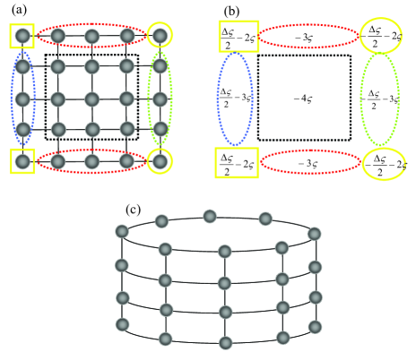
Figure 2: (Color online.) (a) The electric fields with different strengths are applied on the ddot pairs in a periodic structure isolated by the dashed and solid lines with different colors and shapes: $(8k^{\prime}-2)\varsigma/(8k+1)+\Delta\varsigma/2$ (yellow square); $(8k^{\prime}-2)\varsigma/(8k+1)-\Delta\varsigma/2$ (yellow circle); $(8k^{\prime}-4)\varsigma/(8k+1)$ (black dashed box); $(8k^{\prime}-3)\varsigma/(8k+1)$ (red dashed circle); $(8k^{\prime}-3)\varsigma/(8k+1)+\Delta\varsigma/2$ (blue dashed circle); $(8k^{\prime}-3)\varsigma/(8k+1)-\Delta\varsigma/2$ (green dashed circle). (b) By choosing $k=k^{\prime}=0$ for simplicity, we show an example of how to apply electric fields on the ddot pairs for generating a two-dimensional cluster state. (c) The periodic structure of a two-dimensional array of ddot pairs for an alternative method to generate a two-dimensional cluster state by simply applying a global electric field $-3\varsigma$ on the first and last rows, and $-4\varsigma$ for the remaining rows, respectively.

V.2 Cylindrical cluster state

By changing the structure of the array of charge qubits to that shown in Fig. 2(c), we can generate a large two-dimensional cluster state by simply applying global electric fields instead of local electric fields, resulting in an important simplification to the technical challenges of generating cluster states.

From our analysis above we observe that the choice of external electric field strength depends on two factors: the number of connections to nearest neighbors $\nu_{x}+\nu_{y}$ and the extra energy offset due to asymmetry of the two-dimensional structure. The periodic boundary condition $\mathfrak{n}+N=\mathfrak{n}$ dismisses the second factor, and the extra energy offsets of the ddot pairs located on two edge columns cancel each other.

The periodic boundary condition also partially diminishes the first factor and makes the connections of all ddot pairs except for those located on the first and last rows to be $\nu_{x}+\nu_{y}=4$. For those ddots located on the first and last rows, $\nu_{x}+\nu_{y}=3$, and the global electric fields on the two rows are set to be $(8k^{\prime}-3)\varsigma/(8k+1)$ while all the others are set to be $(8k^{\prime}-4)\varsigma/(8k+1).$ For simplicity, choosing $k=k^{\prime}=0$, to generate a two-dimensional cluster state, one only needs to apply an external global electric field $-3\varsigma$ on the first and last rows, and $-4\varsigma$ for the remaining rows, respectively.

V.3 Validity of Ising-like evolution to a cluster state

Our approach is valid if the contribution of the term $\hat{H}_{\text{und}}$ in Eq. (13) to the evolution is negligible. The fidelity of the pure two-dimensional cluster state is

$$F= \left|{}_{\text{ini}}\left\langle{\Psi}\right|{\rm e}^{\text{i}\hat{H}_{\text{eff}}t}{\rm e}^{-\text{i}\hat{H}_{\text{Is}}t}\left|{\Psi}\right\rangle_{\text{ini}}\right|^{2}$$

$$\approx 1-\left(\frac{4N\varsigma tT}{\bar{V}}\right)^{2},$$ (20)

for $N$ qubits, which gives an upper bound of the maximum number of cluster qubits with a fixed fidelity

$$N_{\text{max}}(N^{2})=(1-F)\left(\frac{\bar{V}}{4\varsigma tT}\right)^{2}$$ (21)

for $\bar{V}$ the absolute value of the average energy offset of ddot pairs. In other words, approximating the anisotropic evolution by isotropic Ising-like evolution is valid provided that the total number of qubits does not exceed $N_{\text{max}}$, which depends on the acceptable less-than-unity fidelity $F$.

With the evolution time $t=\pi/4\varsigma$, the fidelity and the maximum number of cluster qubits can be written as $F=1-\left(\pi NT/\bar{V}\right)^{2}$ and $N_{\text{max}}(N^{2})=(1-F)\left(\bar{V}/\pi T\right)^{2}$. For $T=0.1\mu$eV, $\varsigma=10\mu$eV and $\bar{V}\approx 4\varsigma=40\mu$eV (for large $N$), our calculations show that a 2D $162$-qubit cluster state with a high fidelity $F=0.99$ can be produced. For $T=1\mu$eV and $\varsigma=10\mu$eV, $N_{\text{max}}=16$ with a fidelity $F=0.9$ for the 2D cluster state.

VI Conclusions

We have considered deterministic unitary evolution of a cluster state in a charge-qubit structure with charge qubits made of double-dot (ddot) structures. Although periodic evolution into charge-qubit cluster states has been considered before, anisotropy presents a critical yet overlooked challenge. At first anisotropy seems to destroy the opportunity to create cluster states in this way.

We have shown how to circumvent this problem by applying electric field biases to the ddot structures. In the slow-tunneling regime, the effective single-quantized multi-qubit Hamiltonian can be approximated by the Ising-like Hamiltonian. In this case, electric field biases can overcome the challenge of anisotropy. If the electric fields had to be tailored to each ddot charge qubit, or if the field had to be controlled over time, the strategy would be impractical. However, we have shown that a global field over all but the boundary qubits, and five choices of electric field biases on boundary qubits no matter how large the system is, entirely eliminates the problem of anisotropy.

Remarkably, by changing the structure of the array of charge qubits, we can generate a large two-dimensional cylindrical cluster state by simply applying an electric field on the first and last rows, and a different one for the remaining rows, respectively. Compared to previous schemes, no assumption of isotropy for charge qubit couplings is made in our procedure and in fact is shown not to be valid for two-dimensional cluster states. We augment our theoretical analysis of anisotropy by including numerical analysis for the case of GaAs double dots in a two-dimensional lattice. In particular we show that the energy offsets due to anisotropy are noneligible in this case.

For these charge qubits to be useful, noise and decoherence need to be considered. Also the charge qubits considered here periodically evolve into cluster states and then back to their initial states due to the periodic nature of the unitary evolution. Timing becomes critical in such dynamics, or else the interactions that produce the cluster states must be able to be switched off. Measurement-based quantum computing also becomes challenging for such periodically-occurring cluster states. These considerations are the seeds for future study.

- (1) R. Raussendorf and H. J. Briegel, Phys. Rev. Lett. 86, 5188 (2001); R. Raussendorf and H. J. Briegel, Quant. Info. Comp. 2, 344 (2002); R. Raussendorf, D. E. Browne and H. J. Briegel, Phys. Rev. A 68, 022312 (2003).
- (2) H. J. Briegel and R. Raussendorf, Phys. Rev. Lett. 86, 910 (2001).
- (3) P. Walther, K. J. Resch, T. Rudolph, E. Schenck, H. Weinfurter, V. Vedral, M. Aspelmeyer, and A. Zeilinger, Nature 434, 169 (2005).
- (4) T. Tanamoto1, Y.-x. Liu, X. Hu and F. Nori, Phys. Rev. Lett. 102, 100501 (2009).
- (5) T. Tanamoto, Y.-x. Liu, S. Fujita, X. Hu, and F. Nori, Phys. Rev. Lett. 97, 230501 (2006).
- (6) J. Q. You, X.-B. Wang, T. Tanamoto, and F. Nori, Phys. Rev. A75, 052319 (2007).
- (7) T. H. Oosterkamp, T. Fujisawa, W. G. van der Wiel, K. Ishibashi, R. V. Hijman, S. Tarucha, and L. P. Kouwenhoven, Nature 395, 873 (1998).
- (8) P. G. J. van Dongen, Phys. Rev. B49, 7904 (1994).
- (9) L. Livadaru, P. Xue, Z. Shaterzadeh-Yazdi, G. A. DiLabio, J. Mutus, J. L. Pitters, B. C. Sanders, and R. A. Wolkow, arXiv: 0910.1797 (accepted into New Journal of Physics).
- (10) S. Robasziewicz, Phys. Stat. Sol (B) 59, k63 (1973).
- (11) M. Van den Nest, A. Miyake, W. Dür, and H. J. Briegel, Phys. Rev. Lett. 97, 150504 (2006); M. Van den Nest, W. Dür, G. Vidal, H. J. Briegel, Phys. Rev. A75, 012337 (2007).
- (12) J. R. Petta, H. Lu, and A. C. Gossard, Science 327, 669 (2010).