Hydropathy Conformational Letter and its Substitution Matrix
HP-CLESUM: an Application to Protein Structural Alignment

Abstract

Motivation: Protein sequence world is discrete as 20 amino acids (AA) while its structure world is continuous, though can be discretized into structural alphabets (SA). In order to reveal the relationship between sequence and structure, it is interesting to consider both AA and SA in a joint space. However, such space has too many parameters, so the reduction of AA is necessary to bring down the parameter numbers.

Result: We’ve developed a simple but effective approach called entropic clustering based on selecting the best mutual information between a given reduction of AAs and SAs. The optimized reduction of AA into two groups leads to hydrophobic and hydrophilic. Combined with our SA, namely conformational letter (CL) of 17 alphabets, we get a joint alphabet called hydropathy conformational letter (hp-CL). A joint substitution matrix with $(17*2)^{2}$ indices is derived from FSSP. Moreover, we check the three coding systems, say AA, CL and hp-CL against a large database consisting proteins from family to fold, with their performance on the TopK accuracy of both similar fragment pair (SFP) and the neighbor of aligned fragment pair (AFP). The TopK selection is according to the score calculated by the coding system’s substitution matrix. Finally, embedding hp-CL in a pairwise alignment algorithm, say CLeFAPS, to replace the original CL, will get an improvement on the HOMSTRAD benchmark.

Contact*: wangsheng@itp.ac.cn

I Introduction

Proteins fold into specific spatial conformations to perform their biological functions ProteinStructure and there are abundant evidences to show their amino acid (AA) sequences determining the structures Prediction1 . The attempt to find the relationship between structure and sequence is a fundamental task in computational biology SequenceStructure .

Compared to the sequence world which is discrete of 20 AAs, the structure world is continuous, though the local conformational space of a protein backbone fragment is rather limited LocalStructure . The idea of representing the backbone with a string of discrete letters was first observed by Corey and Pauling PaulingAlpha ; PaulingBeta and later refined into the concept of protein secondary structure elements (SSEs). However, segments of a single SSE may vary significantly in their 3D structures, especially for the state coil, which is not a true secondary structure but is a class of conformations that indicate the absence of regular SSEs, say alpha helix or beta strand ConfoLettApp . Although the SSE can be predicted with high accuracy ($\geq$80%) Prediction2 , the description of a protein in terms of its SSEs is not sufficient to capture accurately its 3D geometry Classify .

To overcome this limitation, several groups have proposed the idea that representing protein structures as a series of overlapping fragments, each labeled with a symbol, which defines a structural alphabet (SA) for proteins WodakSA ; BergSA ; ProteinBlock ; LevittSA ; TufferySA ; 3D-BLAST . Such alphabet can be used to predict local structure deBrevern1 ; deBrevern2 ; deBrevern3 , to reconstruct the full-atom representation Reconstruct , to identify the structural motifs MetalBind , to classify protein structures Classify and to search against a database search1 ; search2 . We’ve proposed our SA, namely conformational letter (CL) ConfoLett , which is composed of 17 alphabets and each with 4 residues in length. Our SA is focused on the fast pairwise CLePAPS , multiple CLeMAPS and flexible CLeFAPS structure alignment problems, combined with its substitution matrix CLESUM ConfoLett .

After we discretized the continuous structure world into SAs, it is the time to consider both AA and SA in a joint space. However, such space is too large for about $(20*17)^{2}$ parameters when using the current popular SAs. It is necessary to employ the reduction of AAs ChanRed . Several groups have put forward their reduced AAs either experimentally or computationally. For example, Baker et.al found a five-letter alphabet for 38 out of 40 selected sites of SH3 chain BakerRed ; Wang & Wang WWRed introduced the minimal mismatch principle to reduce the alphabet based on Miyazawa-Jernigan’s residue-residue statistical potential MJmatrix ; Murphy et.al MWLRed approached the same problem using the BLOSUM matrix HHmatrix . Recently, de Brevern et.al proposed to use their SA, namely Protein Blocks ProteinBlock to analyze equivalences between the different kinds of amino acids, then obtained their reduced AAs deBrevernRed .

Here we present a novel reduction method, called entropic clustering ZhengRed . Briefly, given two discrete distributions A and B, merging $a_{i}$ and $a_{j}$ into one group $a_{i\&j}$ will result in a loss of mutual information of A and B. Thus, mutual information $I$ can be naturally chosen as the objective function for optimized clustering. When grouping the 20 AAs into two categories, we’ve got a result of hydrophobic and hydrophilic, which agrees with HP-model Hydropathy exactly. Then we construct a joint substitution matrix HP-CLESUM with $(17*2)^{2}$ indices by the similar means as constructing CLESUM.

The following tests are employed to check and compare different coding systems, namely AA, CL and hp-CL with their corresponding substitution matrix, say BLOSUM, CLESUM and HP-CLESUM. We first compare the TopK accuracy of SFPs (similar fragment pairs) and the neighbor of AFP (aligned fragment pairs) against a large dataset encompassing the protein homologous levels from family to fold according to SCOP SCOP ; then we embed hp-CL into CLeFAPS CLeFAPS , replacing the original CL, to get an improvement against the popular benchmark HOMSTRAD HOMSTRAD .

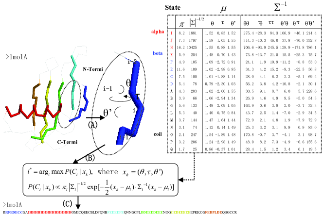
Figure 1: The conversion from 3D protein structure to 1D CL string. (A) Given a sliding window of length four, may we get four contiguous $C_{\alpha}$ atoms, and determine two bending angles $\theta,\theta^{\prime}$ and a torsion angle $\tau$. (B) Select a state which maximize the given data, where each state is a gaussian distribution in the three dimension space of $\theta,\tau,\theta^{\prime}$. (C) Assign the state (letter) to the third place of the four $C_{\alpha}$ atoms, so the $N$ length protein will get $N-3$ letters finally, and we assign the first two and the last position with a ’blank’ letter R.

II Materials and method

II.1 Datasets

We use PDB-SELECT databank PDB-Select to construct our CLs, and use FSSP database FSSP to derive the substitution matrix CLESUM. Particularly, PDB-SELECT contains 1544 non-membrane proteins from PDB PDB with amino acid identity less than 25%. FSSP is based on exhaustive all-against-all structure comparison of the representative protein structures, where the representative set contains no pair which has more than 25% sequence identity. A tree for the fold classification of the 2,860 representative set is constructed by a hierarchical clustering method based on the structural similarities. Family indices of the FSSP are obtained by cutting the tree at levels of 2, 4, 8, 16, 32 and 64 standard deviations above the database average.

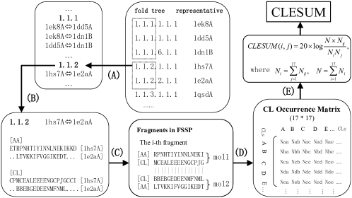
Figure 2: Flowchart of the construction of CLESUM. (A) Collect all pairwise structures with the same first three family indices (DALI Z-Score $\geq$ 8) in the representative set from FSSP. (B) For each pair, extract the alignment. (C) For each alignment, extract the ungapped aligned fragment. Each fragment contains both AAs and CLs. (D) Count the occurrence number of CL duad. For example, Nab means the total number of CL A and B occurred in the alignment. (E) Calculate CLESUM from the occurrence matrix.

II.2 Conformational letter and its substitution matrix

Four contiguous $C_{\alpha}$ atoms, say $i-2$, $i-1$, $i$ and $i+1$, determine two bending angles $\theta,\theta^{\prime}$ and a torsion angle $\tau$ which is the dihedral angle between the two planes of triangles $i-2,i-1,i$ and $i-1,i,i+1$ (see Fig. 1). By using a mixture model for the density distribution of the three angles, the local structural states from PDB-SELECT have been clustered as 17 discrete states (see our previous work ConfoLett for more details). To use our SAs directly for the structural comparison, a score matrix similar as BLOSUM HHmatrix for AAs is desired. In details, we first convert the structures of the representative set from FSSP to their CL strings; then collect all the pair alignments with the same first three family indices (DALI Z-Score $\geq$ 8) (see Fig. 2); finally count all ungapped aligned pairs of CLs to generate the substitution matrix, say CLESUM (Table 1). The total number of structures is 10,047 pairs, consisting of 175,723 fragment pairs and 1,284,750 code pairs.

Table 1: CLESUM: The conformation letter substitution matrix (in 0.05 bit units).

$J$	37
$H$	13	23
$I$	16	18	23
$K$	13	5	21	49
$N$	-2	-34	-11	28	90
$Q$	-44	-87	-62	-24	32	90
$L$	-32	-62	-41	-1	8	26	74
$G$	-21	-51	-34	-13	-8	8	29	69
$M$	16	-4	1	12	7	-7	5	21	61
$B$	-57	-96	-74	-50	-11	12	-12	13	-13	51
$P$	-34	-60	-49	-36	-3	7	-12	5	8	42	66
$A$	-23	-45	-31	-19	10	16	-11	-6	-2	20	35	73
$O$	-24	-55	-34	5	15	-13	-4	-1	5	-12	4	25	104
$C$	-43	-77	-56	-33	-5	29	0	-4	-12	7	4	13	3	53
$E$	-93	-127	-108	-84	-43	-6	-21	-22	-47	15	-5	-25	-48	3	36
$F$	-73	-107	-88	-69	-32	3	-16	-5	-33	7	0	-20	-30	20	26	50
$D$	-88	-124	-105	-81	-44	14	-22	-31	-49	13	-10	-17	-42	21	22	21	52
	$J$	$H$	$I$	$K$	$N$	$Q$	$L$	$G$	$M$	$B$	$P$	$A$	$O$	$C$	$E$	$F$	$D$

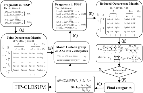
Figure 3: Flowchart of entropic clustering on the joint space of both AAs and CLs. (A) For each fragment in FSSP, count the pairwise number of joint occurrence. For example, Ndaac means the total pairwise number of ’da’ with ’ac’, in each duad the former is CL and the latter is AA. (B) Use Monte Carlo to randomly group 20 AAs into two categories. (C) Given an AA category, assign each AA to its group. (D) Calculate the reduced occurrence matrix, here Nd0a1 means the total pairwise number of ’d0’ with ’a1’, in each duad the former is CL and the latter is AA’s tag. (E) Calculate the mutual information of the reduced matrix. (F) If the categories which maximize $I$ have been found, break the Monte Carlo recursion. (G) Calculate the HP-CLESUM.

II.3 Entropic clustering

From FSSP, which contains also the AA information, it is possible to construct a substitution matrix in the joint space of the structure and sequence. However, such matrix would have about (17$\times$20)$\times$(17$\times$20) parameters (Fig. 3(A)). If we group the 20 AAs into two clusters, then the parameters of the matrix are reduced to (17$\times$2)$\times$(17$\times$2).

Generally, the mutual information $I$ of two discrete distribution ($A$ and $B$) is defined as,

$$I=\sum\limits_{a,b}^{a\in A,b\in B}p(a,b)\log\frac{p(a,b)}{p(a)p(b)}.$$ (1)

If we cluster $a_{i}$ and $a_{j}$ into $a_{i\&j}$ leads to

$$p(a_{i\&j}) = p(a_{i})+p(a_{j}),$$

$$p(a_{i\&j},b) = p(a_{i},b)+p(a_{j},b).$$ (2)

The difference between values of $I$ after and before clustering is given by

$${[p(a_{i},b)+p(a_{j},b)]\log\frac{{p(a_{i},b)+p(a_{j},b)}}{{[p(a_{i})+p(a_{j})]p(b)}}}$$

$${-p(a_{i},b)\log\frac{{p(a_{i},b)}}{{p(a_{i})p(b)}}-p(a_{j},b)\log\frac{{p(a_{j},b)}}{{p(a_{j})p(b)}}}$$ (3)

which, by introducing

$$x_{i} = \frac{p(a_{i},b)}{p(a_{i})},$$

$$\omega_{i} = \frac{p(a_{i})}{p(a_{i})+p(a_{j})},$$ (4)

and their analogs $x_{j}$ and $\omega_{j}$, then defining $\left\langle{F(x)}\right\rangle=\omega_{i}F(x_{i})+\omega_{j}F(x_{j})$ and $F(\left\langle x\right\rangle)=F(\omega_{i}x_{i}+\omega_{j}x_{j})$ where $\omega_{i}+\omega_{j}=1$. We may now see that Eq. (II.3) is proportional to $f(\left\langle x\right\rangle)-\left\langle{f(x)}\right\rangle$ with $f(x)=x\log x$. From the Jensen’s inequality, for the convex function $x\log x$ here we have $f(\left\langle x\right\rangle)\leq\left\langle{f(x)}\right\rangle$, so $I$ never increases after any step of clustering.

That is to say, merging any two members into one cluster will result in a loss of mutual information. To make the loss of mutual information as small as possible, $I$ should be maximized, so it can be naturally chosen as the objective function during clustering. We call this approach entropic clustering ZhengRed . If we partition $n$ objects into $m_{1}$ and $m_{2}$ classes, where $m_{2}>m_{1}$, it is easy to prove that the maximal $I$ at $m_{2}$ is always greater than the maximal $I$ at $m_{1}$ ConfoLettApp .

Now turning back to our substitution matrix in the joint space, we may define the average mutual information as follows like BLOSUM,

$$I=\sum\limits_{X,Y}{P_{XY}\log\frac{{P_{XY}}}{{P_{X}P_{Y}}}},$$ (5)

where $X$ and $Y$ means a joint state of CL and AA (either reduced or not). Given a clustering group may we calculate its $I$ based on Eq. (5) and according to entropic clustering we should get a categories which maximize $I$ (Fig. 3(F)).

III Result

III.1 Joint substitution matrix of conformational letters and reduced amino acids

For clustering the 20 AAs into two categories, the Monte Carlo finds AVCFIWLMY and DEGHKNPQRST as the groups, which is just the hydrophobic and hydrophilic cluster Hydropathy . Such enlarged CLs are called hp-CLs.

Table 2: CLESUM-hh (lower left) and CLESUM-pp (upper right) (in units of 0.05 bit): ’black dot’ and ’white cycle’ to indicate the the CLs with different hydropathy AA types.

	$\mathring{J}$	$\mathring{H}$	$\mathring{I}$	$\mathring{K}$	$\mathring{N}$	$\mathring{Q}$	$\mathring{L}$	$\mathring{G}$	$\mathring{M}$	$\mathring{B}$	$\mathring{P}$	$\mathring{A}$	$\mathring{O}$	$\mathring{C}$	$\mathring{E}$	$\mathring{F}$	$\mathring{D}$
	45	19	24	19	3	-41	-27	-13	21	-49	-32	-21	-22	-37	-79	-62	-73	$\mathring{J}$
		30	24	7	-31	-76	-60	-45	-5	-84	-57	-46	-55	-69	-113	-92	-108	$\mathring{H}$
$\dot{J}$	40		31	27	-6	-57	-38	-28	3	-64	-44	-30	-31	-48	-93	-72	-89	$\mathring{I}$
$\dot{H}$	18	30		57	39	-16	5	-8	20	-43	-33	-12	6	-24	-66	-52	-64	$\mathring{K}$
$\dot{I}$	20	26	30		94	39	15	-5	11	-12	-1	14	16	0	-35	-25	-31	$\mathring{N}$
$\dot{K}$	18	14	28	59		95	33	14	-4	10	8	21	-14	33	3	13	20	$\mathring{Q}$
$\dot{N}$	-2	-16	3	40	108		76	35	12	-12	-8	-3	-4	7	-11	-5	-14	$\mathring{L}$
$\dot{Q}$	-41	-110	-67	-19	27	109		80	33	7	9	-1	-4	1	-11	5	-17	$\mathring{G}$
$\dot{L}$	-33	-58	-37	10	8	30	86		69	-6	13	4	9	-4	-32	-21	-34	$\mathring{M}$
$\dot{G}$	-22	-48	-35	-10	-11	2	40	80		64	55	31	-4	13	20	14	25	$\mathring{B}$
$\dot{M}$	24	7	9	16	10	-5	9	25	71		74	38	7	9	3	7	0	$\mathring{P}$
$\dot{B}$	-64	-99	-82	-61	-7	15	-3	31	-12	59		75	31	20	-16	-11	-4	$\mathring{A}$
$\dot{P}$	-31	-57	-47	-39	-1	13	-21	4	13	45	76		107	10	-37	-24	-32	$\mathring{O}$
$\dot{A}$	-19	-36	-26	-25	13	11	-24	-10	-6	21	42	85		60	12	28	33	$\mathring{C}$
$\dot{O}$	-9	-37	-18	-14	25	29	-8	13	11	13	36	32	121		45	32	30	$\mathring{E}$
$\dot{C}$	-49	-87	-67	-45	-17	36	-8	-7	-24	10	7	17	14	62		58	30	$\mathring{F}$
$\dot{E}$	-110	-138	-126	-98	-56	-5	-24	-22	-58	24	3	-23	-22	9	44		61	$\mathring{D}$
$\dot{F}$	-92	-131	-105	-106	-46	3	-24	-4	-45	10	3	-24	5	29	34	61
$\dot{D}$	-98	-138	-111	-95	-67	33	-20	-36	-66	14	-10	-22	-31	26	30	28	63
	$\dot{J}$	$\dot{H}$	$\dot{I}$	$\dot{K}$	$\dot{N}$	$\dot{Q}$	$\dot{L}$	$\dot{G}$	$\dot{M}$	$\dot{B}$	$\dot{P}$	$\dot{A}$	$\dot{O}$	$\dot{C}$	$\dot{E}$	$\dot{F}$	$\dot{D}$

Table 3: CLESUM-hp (row-column) (in units of 0.05 bit).

$\mathring{J}$	27	3	6	3	-3	-47	-38	-31	6	-65	-40	-28	-8	-50	103	-84	101
$\mathring{H}$	10	14	10	-1	-25	-86	-69	-60	-11	-112	-67	-46	-35	-87	-140	-126	-139
$\mathring{I}$	13	9	13	13	-9	-64	-44	-40	-7	-80	-59	-30	-21	-65	-119	-108	-121
$\mathring{K}$	11	-2	12	36	23	-37	-15	-19	4	-48	-40	-25	8	-40	-94	-77	-93
$\mathring{N}$	-12	-48	-25	4	76	16	-10	-8	-1	-9	-6	3	15	-13	-46	-41	-59
$\mathring{Q}$	-50	-94	-66	-37	14	70	11	5	-13	16	5	12	-9	15	-14	-11	-5
$\mathring{L}$	-35	-65	-47	-8	12	25	65	17	-3	-13	-8	-10	10	-4	-26	-24	-29
$\mathring{G}$	-20	-54	-35	-15	-17	6	16	52	12	-5	0	-8	21	-5	-31	-13	-37
$\mathring{M}$	11	-13	-5	4	12	-1	-3	9	47	-17	4	-4	13	-16	-54	-41	-54
$\mathring{B}$	-54	-95	-75	-53	-19	-1	-19	5	-21	34	35	18	4	6	-2	-3	-1
$\mathring{P}$	-34	-62	-50	-36	-6	0	-19	4	1	21	53	32	17	-1	-22	-16	-27
$\mathring{A}$	-26	-49	-37	-24	7	6	-19	-8	-7	2	26	66	26	2	-37	-30	-31
$\mathring{O}$	-35	-62	-43	4	9	-21	-7	-4	-3	-35	-12	0	67	-22	-69	-55	-57
$\mathring{C}$	-42	-74	-57	-36	-10	30	-4	-8	-12	-3	1	7	9	42	-14	0	2
$\mathring{E}$	-81	-116	-95	-80	-44	-6	-23	-24	-43	12	-1	-21	-19	8	25	18	14
$\mathring{F}$	-64	-95	-79	-62	-20	2	-15	-9	-30	4	5	-18	2	21	14	33	14
$\mathring{D}$	-84	-114	-100	-79	-30	20	-25	-32	-45	11	-3	-17	-29	23	9	9	34
	$\dot{J}$	$\dot{H}$	$\dot{I}$	$\dot{K}$	$\dot{N}$	$\dot{Q}$	$\dot{L}$	$\dot{G}$	$\dot{M}$	$\dot{B}$	$\dot{P}$	$\dot{A}$	$\dot{O}$	$\dot{C}$	$\dot{E}$	$\dot{F}$	$\dot{D}$

The substitution matrix of hp-CLs is called HP-CLESUM, this symmetry matrix can be divided into three sub-matrices: CLESUM-hh, CLESUM-pp, and CLESUM-hp. The first two, shown in Table 2, correspond to the same hydropathy aligned amino acid types (i.e., h-h and p-p). The third, shown in Table 3, corresponds to the different hydropathy types h-p. As expected, compared with the original CLESUM (Table 1), elements of CLESUM-hh and CLESUM-pp generally become larger in absolute values, and those of CLESUM-hp show the opposite tendency. The tendency is stronger for letters dominated by helices or sheets.

Table 4: TopK accuracy check with different strategies, from TopK SFP check (left part) to TopK AFP’s neighbor check (right part); different coding systems, from AA (A%), CL (C%) to hp-CL (H%); different homologous level, from family (Fam), superfamily (Sup) to fold; and different SFP length $L$, from 6, 12 to 18.

			TopK SFP’s Accuracy																	TopK AFP’s Neighbor Accuracy
Level	TopK		$L=6$				$L=12$				$L=18$				Self(9-18)∗			TopK		$L=6$				$L=12$				$L=18$
			A%	C%	H%		A%	C%	H%		A%	C%	H%		C%	H%				A%	C%	H%		A%	C%	H%		A%	C%	H%
Fam	1		53.1	63.1	68.0		62.4	74.4	77.6		62.4	74.3	77.1		73.1	75.5		1		25.8	41.4	46.3		46.1	69.7	74.2		62.4	86.0	88.5
	5		74.4	86.7	88.9		79.4	90.7	92.3		80.1	91.2	92.4		90.1	91.6		2		35.1	53.3	59.0		55.8	79.3	83.4		71.0	91.7	93.7
	10		82.0	93.1	94.4		85.7	95.4	96.2		86.6	96.0	96.6		95.2	96.0		3		41.1	59.9	65.9		61.4	83.4	87.3		75.4	93.9	95.6
	20		89.1	97.1	97.8		91.8	98.2	98.6		92.8	98.4	98.8		98.0	98.5		4		45.7	64.4	70.5		65.2	85.9	89.6		78.3	95.0	96.6
Sup	1		39.1	48.7	52.4		44.8	58.3	61.8		43.8	58.2	61.4		56.2	59.4		1		22.5	36.3	40.6		39.7	63.9	68.0		56.6	83.3	85.8
	5		58.2	73.7	76.7		62.4	79.2	81.8		63.0	79.7	81.5		78.4	80.3		2		31.0	47.9	52.9		48.9	73.9	77.6		65.1	89.8	91.7
	10		67.0	83.1	85.3		71.1	87.3	88.9		72.7	87.9	89.4		86.9	88.5		3		36.7	54.7	59.8		54.2	78.5	82.2		69.5	92.3	93.9
	20		77.2	90.5	91.8		81.0	93.5	94.5		82.8	94.2	95.0		93.5	94.4		4		41.1	59.4	64.7		57.9	81.4	84.9		72.5	93.7	95.2
Fold	1		13.9	26.8	29.7		17.0	33.8	36.7		17.0	33.5	35.6		31.9	34.2		1		10.7	24.8	27.0		20.0	46.6	49.8		32.2	68.4	70.7
	5		28.8	50.3	54.2		33.2	57.0	60.2		34.2	58.6	60.7		57.4	59.6		2		17.3	35.1	38.6		28.3	57.8	61.4		41.5	77.4	79.4
	10		39.5	63.6	66.7		45.7	70.5	73.0		48.4	74.1	75.4		72.5	74.2		3		22.3	41.9	46.0		33.7	63.8	67.6		46.9	81.5	83.5
	20		55.8	77.2	79.4		62.3	84.5	86.3		66.3	87.0	87.8		85.9	87.0		4		26.4	46.9	51.4		37.8	67.8	71.6		51.1	84.3	86.2
∗: Self(9-18) means the application of self-adaptive strategy CLeFAPS of the SFP’s length $L$ from 9 to 18.

III.2 Comparison between different coding systems

III.2.1 Overview

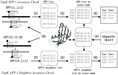
Figure 4: TopK accuracy check procedure. (A) Select a pair of structures and aligned by MATT, resulting a series of AFPs. (B) Encode the pairwise structures, the coding system may be AA or SA. (C) Search for any SFPs with length $L$ according to a certain coding system. (D) Sort these SFPs in descending order, the score is calculated by the corresponding substitution matrix. (E) Check whether there exists a correct SFP within TopK. (F) Search for any possible neighbor of a given AFP whose length is over $L$ against the other string. (G) Sort these AFP’s neighbors. (H) Check their accuracy.

A coding system in protein structure is defined as an alphabet combined with its corresponding substitution matrix. Amino acids (AA) or all kinds of SAs can be treated as coding systems, so long as the alphabet has its substitution matrix. We’ll compare the performance of the following three ones, namely AA, CL and hp-CL, based on their TopK accuracy against a benchmark (Fig. 4). The difference between SFP and AFP is, we use SFPs to describe all local similar fragment pairs, while AFPs is a subset of SFPs that each of them should be in the final alignment CLeFAPS .

Note if the length of an AFP, say $Len$ is longer than $L$, we’ll check each positions and the total number is $Len-L+1$; if $Len$ is shorter than $L$, we just skip this AFP. As a result, the TopK SFPs’ accuracy of a single pair of structures is a 0 or 1 measure, that is to say, within TopK we find a correct SFP or not. While the TopK neighbor of AFP’s accuracy is calculated by summing all correct positions found in any AFPs then dividing the total valid positions, the result is between 0.0 to 1.0.

The benchmark we use is divided in three levels: family, superfamily and fold according to SCOP SCOP . In family set, we use all SCOP families which have 2 to 25 members in ASTRAL 40% compendium ASTRAL and the total pair number is 21,039. In superfamily and fold, it is convenient to use SABmark SABmark instead of using ASTRAL 40% because SABmark is systematically arranged and elaborately checked at both superfamily and fold level. The superfamily set contains 3,645 domains sorted into 426 subsets and the fold set (or be called twilight zone TwilightZone ) contains 1,740 domains sorted into 209 subsets, where each subsets contain between 3 to 25 structures. The superfamily set contains 18,724 structure pairs and the fold set contains 10,306. We apply MATT MATT to conduct all-against-all pairwise alignment within each family or subset as our gold standard.

III.2.2 Performance

Table 4 shows that, hp-CL performs best while CL follows the second, both of them outperforms 10% to 100% than AA. For details, with the increase of TopK and length $L$, the accuracy of all coding systems grows better, while from family to fold level, the accuracy declines. It is surprising that at fold level, the accuracy of hp-CL outperforms AA more than 50% at the TopK SFP accuracy test and more than 100% at the TopK neighbor of AFP test, while in the latter, hp-CL got the average accuracy at about 71% given $L=18$ from the Top-1 highest neighbor of an AFP. Such feature may be applied to construct the Highest Similarity Fragment Block (HSFB) during the multiple structure alignment ConfoLettApp . Given a seed structure and a certain position, if this position got many high score neighbors in other structures, may we say that this block (consisting the seed position and its neighbors) has a more probable chance in the final multiple alignment.

Moreover, we’ve shown the effectiveness of parameter self-adaptive strategy to create the SFP-list in CLeFAPS . At most cases self-adaptive strategy is compatible with fixed parameters, while the size of the SFP-list can be controlled empirically to about O(n²/LEN_H/6) with the LEN_H=9 (Fig. 5). However, its hard to control the balance between the size of the SFP-list and the threshold of SFP generated with fixed parameters strategy. Actually, the data of fixed length used in Table 4 is considered all O(n²) SFPs, then to select TopK; we’ve tested different SFP thresholds, if it is set too high there’ll lead to blank or few SFP-list while if it is set too loose then the SFP-list will be too much (data not shown).

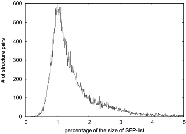
Figure 5: Histogram of the percentage of SFP-list’s size to the search space (moln1*moln2) between all homologous levels (from family to fold) under the self-adaptive strategy, where the moln1 (moln2) is the first (second) structure’s size. The peak value is about 1.045% and the mean value is about 1.5505%. The total pair count is 50,069.

Finally, we may get the conclusion that, during structure comparison, the only consideration of the TopK highest SFPs to built the initial alignment is feasible from family level to fold, so long as the coding system is specific enough. Also the employment of parameter self-adaptive strategy to generate SFPs is effective and economic.

III.3 Implement of hydropathy conformational letters to structural alignment

We embed hp-CL to the pairwise protein structural alignment problem under the framework of CLeFAPS CLeFAPS . Particularly, we first transform each structures to its hp-CL strings; then search for both highly specific SFPs (SFP_H) that have a high HP-CLESUM score to build an initial alignment from the best TM-score TMscore SFP within TopK, and highly sensitive SFPs (SFP_L) that have a low HP-CLESUM score (must above 0) to refine the alignment through fuzzy-add strategy. These two SFP-lists can be generated simultaneously CLePAPS ; finally we apply an elongation based on Vect-score to collect local flexible fragments.

Table 5: Alignment accuracy metric on HOMSTRAD

Metric	CLeFAPS(CL)	CLeFAPS(hp-CL)	MATT
C/LOA1	0.929	0.939	0.948
C/LOR2	0.898	0.907	0.831
1: Correct/(Length of the algorithm).
2: Correct/(Length of the reference).

HOMSTRAD is a database of protein structural alignments for homologous families HOMSTRAD . Its alignments were generated using structural alignment programs, then followed by a manual scrutiny of individual cases. There are totally 1033 families (633 at pairwise level). We’ll show the improvement based on hp-CL as the coding systems instead of CL under the same algorithm, say CLeFAPS, in Table 5.

IV Discussion and future work

To explore the joint space of both AAs and SAs, entropic clustering is a simple but effective approach. In this work, only the reduction of AAs is considered, while we may also reduce CLs and AAs simultaneously while balancing the accuracy and the parameter numbers. For example, if reducing the CL to 9 letters, (actually, from Fig. 1, there are 4 codes for helix which can be grouped to one cluster, the same as sheet.) we may then consider up to four AA cluster instead of two, while the total alphabet number is about the same as hp-CL.

It is interesting that, hp-CL can be applied during the situation we know only a little information about the AA sequence of the structure, i.e., the hydropathy features, or even none. That is true because, from the knowledge of protein design ProteinDesign2 ; ProteinDesign1 , the hydropathy patterns from a 3D structure may probably be deduced. Then the usage of hp-CLs and HP-CLESUM that consider the hydropathy patterns will get a more accurate result than CLs and CLESUM that only consider the 3D structure.

We also verify a basic idea in CLeFAPS, i.e., self-adaptive strategy to generate SFPs, that we needn’t consider the parameters to deal with different purposes and different proteins. The result showed its accuracy is maintained well and the SFP-list size is controlled in O(n²/LEN_H/6) while its hard to judge the balance between accuracy and size with fixed parameters.

TopK accuracy check has demonstrated the basic strategy of both CLePAPS and CLeFAPS efficient, which only considers TopK highest SFPs to built the initial alignment. Moreover, TopK accuracy check is an effective approach to measure the coding systems against a reference dataset, especially to judge the substitution matrix. If a coding system is good enough, it should rank those SFPs with highly specificities top enough among other SFPs. In a future work, we’ll use this approach to test the current available SAs based on their performance for finding specific SFPs. Also we can do the comparison between SAs and RMSD values or some p-values derived from RMSD. Such comparison between 1D coding systems with 3D expression will show the effectiveness of SAs because they contain the statistic information from the database CLePAPS .

References

- (1) Chothia, C. (1984). Principles that determine the structure of proteins. Annu. Rev. Biochem. 53:537-572.
- (2) Baker, D. & Sali, A. (2001). Protein structure prediction and structural genomics. Science 294:93-96.
- (3) Jones, D. (1999). Protein secondary structure prediction based on position-specific scoring matrices. J. Mol. Biol. 292:195-202.
- (4) Eidhammer, I., Jonassen, I. & Taylor,W.R. (2000). Structure comparison and structure patterns. J. Comput. Biol. 7:685-716.
- (5) Offmann, B., Tyagi, M., & de Brevern, A.G. (2007). Local protein structures. Current Bioinformatics 2:165-202.
- (6) Pauling, L., Corey, R. & Branson, H. (1951). The structure of proteins: two hydrogen-bonded helical configurations of the polypeptide chain. Proc. Natl Acad. Sci. USA. 37:205-234.
- (7) Pauling, L. & Corey, R. (1951). Configurations of polypeptide chains with favored orientations around single bonds: two new pleated sheets. Proc. Natl Acad. Sci. USA. 37:729-740.
- (8) Rooman, M., Rodriguez, J. & Wodak, S. (1990). Automatic definition of recurrent local structure motifs in proteins. J. Mol. Biol. 213:327-336.
- (9) Fetrow, J., Palumbo, M. & Berg, G. (1997). Patterns, structures, and amino acid frequency in structural building blocks, a protein secondary structure classification scheme. Proteins 27:249-271.
- (10) de Brevern, A., Etchebest, C. & Hazout, S. (2001). Bayesian probabilistic approach for predicting backbone structures in terms of protein blocks. Proteins 41:271-287.
- (11) Kolodny, R., Koehl, P., Guibas, L. & Levitt, M. (2002). Small libraries of protein fragments model native protein structures accurately. J. Mol. Biol. 323:297-307.
- (12) Camproux, A., Gautier, R. & Tuffery, P. (2004). A hidden Markov model derived structural alphabet for proteins. J. Mol. Biol. 339:591-605.
- (13) Tung, C.H., Huang, J.W. & Yang, J.M. (2007).Kappa-alpha plot derived structural alphabet and BLOSUM like substitution matrix for rapid search of protein structure database. Genome Biol. 8:R31.1-R31.16.
- (14) Zheng, W.M. & Liu, X. (2005). A protein structural alphabet and its substitution matrix CLESUM. Lecture notes in Bioinformatics 3680 (eds. C. Priami and A. Zelikovsky), Springer Verlag, Berlin 2005:59-67.
- (15) Camproux, A., de Brevern, A., Hazout, S. & Tuffery, P. (2001). Exploring the use of a structural alphabet for structural prediction of protein loops. Theor. Chem. Acc. 106:28-35.
- (16) Fourrier, L., Benros, C. & de Brevern, A. (2004). Use of a structural alphabet for analysis of short loops connecting repetitive structures. BMC Bioinformatics 5:58-71.
- (17) Etchebest, C., Benros, C., Hazout, S. & de Brevern, A. (2005). A structural alphabet for local protein structures: improved prediction methods. Proteins 59:810-827.
- (18) Maupetit, J., Gautier, R. & Tuffery, P. (2006). SABBAC: online structural alphabet-based protein backbone reconstruction from alpha-carbon trace. Nucleic Acids Res. 34:W147-W151.
- (19) Dudev, M. & Lim, C. (2007). Discovering structural motifs using a structural alphabet application to magnesium-binding sites. BMC Bioinformatics 8:106-117.
- (20) Le, Q., Pollastri, G. & Koehl, P. (2009). Structural alphabets for protein structure classification: a comparison study. J. Mol. Biol. (2009), doi:10.1016/j.jmb.2008.12.044.
- (21) Guyon, F., Camproux, A.C., Hochez, J. & Tuffery, P. (2004). SA-Search: a web tool for protein structure mining based on a structural alphabet. Nucleic Acids Res. 32:W545-W548.
- (22) Yang, J.M. & Tung, C.H. (2006). Protein structure database search and evolutionary classification. Nucleic Acids Res. 34:3646-3659.
- (23) Zheng, W.M. (2008). The use of a conformational alphabet for fast alignment of protein structures. Lecture notes in Bioinformatics 4983 (eds. C. Priami and A. Zelikovsky), Springer Verlag, Berlin 2008:331-342.
- (24) Wang, S. & Zheng, W.M. (2009). CLePAPS: fast pair alignment of protein structures based on conformational letters. J. Bioinform. Comput. Biol. 6:347-366.
- (25) Liu, X., Zhao, Y.P. & Zheng, W.M. (2009). CLeMAPS: multiple alignment of protein structures based on conformational letters. Proteins 71:728-736.
- (26) Wang, S. (2009). CLeFAPS: fast flexible alignment of protein structures based on conformational letters.
- (27) Chan, H.S. (1999). Folding alphabets. Nat. Struct. Biol. 6:994-996.
- (28) Riddle, D.S., Santiago, J.V., Bray-Hall, S.T., Doshi, N., Grantcharova, V.P., Yi, Q. & Baker, D. (1997). Functional rapidly folding proteins from simplified amino acid sequences. Nat. Struct. Biol 4:805-809.
- (29) Wang, J. & Wang, W. (1999). A computational approach to simplifying the protein folding alphabet. Nat. Struct. Biol. 6:1033-1038.
- (30) Miyazawa, S. & Jernigan, R.L. (1993). A new substitution matrix for protein sequence searches based on contact frequencies in protein structures. Protein Eng. 6:267-278.
- (31) Murphy, L.R., Wallqvist, A. & Levy, R.M. (2000). Simplified amino acid alphabets for protein fold recognition and implications for folding. Protein Eng. 13:149-152.
- (32) Henikoff, S. & Henikoff, J.G. (1992). Amino acid substitution matrices from protein blocks. Proc. Natl. Acad. Sci. USA. 89:10915-10919.
- (33) Etchebest, C., Benros, C., Bornot, A., Camproux, A., & de Brevern, A. (2007). A reduced amino acid alphabet for understanding and designing protein adaptation to mutation. Eur. Biophys. J. 36:1059-1069.
- (34) Zheng, W.M. (2004). Clustering of amino acids for protein secondary structure prediction. J. Bioinfor. Comp. Biol. 2:333-342.
- (35) Gaboriaud, C., Bissery, V., Benchetrit, T. & Mornon, J.P. (1987). Hydrophobic cluster analysis: an efficient new way to compare and analyse amino acid sequences. FEBS Lett. 224:149-155.
- (36) Hobohm, U. & Sander, C. (1994). Enlarged representative set of protein structures. Protein Sci. 3:522-524.
- (37) Berman, H.M., Westbrook, J., Feng, Z., Gilliland, G., Bhat, T.N., Weissig, H., Shindyalov, I.N. & Bourne, P.E. (2000). The protein data bank. Nucleic Acids Res. 28:235-242.
- (38) Holm, L. & Sander, C. (1996). The FSSP database: fold classification based on structure-structure alignment of proteins. Nucleic Acids Res. 24:206-209.
- (39) Zhang, Y. & Skolnick, J. (2004). Scoring function for automated assessment of protein structure template quality. Proteins 57:702-710.
- (40) Hecht, M.H., Das, A., Go, A., Bradley, L.H. & Wei, Y. (2004). De novo proteins from designed combinatorial libraries. Protein Sci. 13:1711-1723.
- (41) Kamtekar, S., Schiffer, J.M., Xiong, H., Babik, J.M. & Hecht, M.H. (1993). Protein design by binary patterning of polar and nonpolar amino acids. Science 262:1680-1685.
- (42) Mizuguchi, K., Deane, C., Blundell, T.L. & Overington, J. (1998). HOMSTRAD: a database of protein structure alignments for homologous families. Protein Sci. 11:2469-2471.
- (43) VanWalle, I., Lasters, I. & Wyns, L. (2005). SABmark: a benchmark for sequence alignment that covers the entire known fold space. Bioinformatics 21:1267-1268.
- (44) Kolodny, R., Koehl, P. & Levitt, M. (2005). Comprehensive evaluation of protein structure alignment methods: Scoring by geometric measures. J. Mol. Biol. 346:1173-1188.
- (45) Menke, M., Berger, B. & Cowen, L. (2008). Matt: local flexibility aids protein multiple structure alignment. PLoS Comput. Biol. 4(1): e10.
- (46) Murzin, A.G., Brenner, S.E., Hubbard, T. & Chothia,C. (1995). SCOP:a structural classification of proteins database for the investigation of sequences and structures. J. Mol. Biol. 247:536-540.
- (47) Chandonia, J.M., Hon, G., Walker, N.S., Conte, L.L., Koehl, P., Levitt, M. & Brenner, S.E. (2004). The ASTRAL compendium in 2004. Nucleic Acids Res. 32:D189-D192.
- (48) Doolittle, R.F. (1981). Similar amino acid sequences: chance or common ancestry. Science 214:149-159.