Testing minimal lepton flavor violation with
extra vector-like leptons at the LHC

Abstract

Models of minimal lepton flavor violation where the seesaw scale is higher than the relevant flavor scale predict that all lepton flavor violation is proportional to the charged lepton Yukawa matrix. If extra vector-like leptons are within the reach of the LHC, it will be possible to test the resulting predictions in ATLAS/CMS.

I Introduction

Measurements of flavor changing processes in meson decays are all in agreement with the Standard Model (SM) predictions. Such a situation is not expected if there is new physics at the TeV scale, unless its flavor structure resembles that of the SM. The strongest suppression of the new physics flavor effects would arise if all new flavor couplings were proportional to the SM Yukawa couplings, $Y^{U}$ and $Y^{D}$, an idea that became known as “minimal flavor violation” (MFV) D'Ambrosio:2002ex ; Hall:1990ac ; Chivukula:1987py ; Buras:2000dm ; Kagan:2009bn and which applies, for example, in several known supersymmetric models, such as gauge mediation.

As concerns the lepton sector, the fact that no flavor changing neutral current (FCNC) decays of charged leptons have been observed suggests that a similar principle – minimal lepton flavor violation (MLFV) – might apply Cirigliano:2005ck ; Cirigliano:2006su ; Cirigliano:2006nu ; Branco:2006hz ; Chen:2008qg . The existence of neutrino masses, however, implies that there are at least two possible scenarios of MLFV. It is quite likely that the seesaw mechanism, involving heavy singlet fermions with masses $m_{N}\gg m_{Z}$, is responsible for the generation of the light neutrino masses. If the mass scale $m_{N}$ is lower than the scale of flavor dynamics, then there could be three relevant flavor violating matrices: The Yukawa matrix of the charged leptons $Y^{E}$, the Yukawa matrix of the neutrinos $Y^{N}$, and the heavy neutrino mass matrix $M_{N}$. If $m_{N}$ is higher than the scale of flavor dynamics, then MLFV requires that all low energy flavor violating couplings are proportional to $Y^{E}$. In this work, we use the term MLFV for the latter scenario only.

While the high $p_{T}$ experiments at the LHC, ATLAS and CMS, have not been constructed as flavor machines, the fact that they can identify electrons and muons with high precision makes them potentially powerful probes of lepton flavor physics. If new particles, with masses within the reach of the LHC, decay into the SM charged leptons, then ATLAS and CMS are uniquely capable of probing detailed features of the new particles, which may be crucial in understanding the underlying theory. This has been demonstrated for various classes of supersymmetric models Allanach:2008ib ; Feng:2007ke ; Feng:2009yq ; Feng:2009bd ; Buras:2009sg . (Implications of quark-related MFV for LHC phenomenology have also been explored Gresham:2007ri ; Grossman:2007bd ; Dittmaier:2007uw ; Hiller:2008wp ; Burgess:2009wm ; Hiller:2009ii ; Arnold:2009ay .)

In this work, we focus on an extension of the SM where there are heavy – but still within the reach of the LHC – vector-like doublet-leptons. MLFV gives strong predictions concerning the spectrum and the couplings of such new leptons. We analyze how, and to what extent, ATLAS and CMS can test the MLFV hypothesis with such new particles.

The plan of this paper goes as follows. In Section II we present our theoretical framework. In Section III we describe the LHC phenomenology. In Section IV we analyze the lessons concerning minimal flavor violation that can be drawn from the ATLAS/CMS measurements.

II The theoretical framework

The SM leptons include the lepton $SU(2)$-doublets $L_{L}$ and the charged lepton $SU(2)$-singlets $E_{R}$. We assume that, in addition to the SM leptons, there exist vector-like leptons, $\chi_{L}$ and $\chi_{R}$, which are $SU(2)$-doublets and carry hypercharge $-1/2$ (so that the electric charges of the two members in each doublet are $0$ and $-1$). The most general Yukawa and mass terms of the leptonic sector in this extended framework are the following:

$${\cal L}_{\rm leptons}=-Y^{E}_{ij}\overline{L_{L}^{i}}\phi E_{R}^{j}-(m_{2}/v)Y^{\chi}_{ij}\overline{\chi_{L}^{i}}\phi E_{R}^{j}-M_{2}X^{\chi}_{ij}\overline{\chi_{L}^{i}}\chi_{R}^{j}-M_{1}X^{L}_{ij}\overline{L_{L}^{i}}\chi_{R}^{j}.$$ (1)

where $v=\langle\phi\rangle$, and $m_{2},M_{1},M_{2}$ have dimension of mass. The first two terms are Yukawa couplings and the last two bare mass terms. We introduce the ratio $m_{2}/v$ into the second term for later convenience. We assume that the electroweak symmetry breaking parameters $v$ and $m_{2}$ are smaller than the electroweak symmetry conserving ones, $M_{1}$ and $M_{2}$.

II.1 The models

To implement the MLFV principle, we need to assign the various fields to representations of the lepton flavor symmetry

$$G_{\rm LF}=SU(3)_{L}\times SU(3)_{E}.$$ (2)

By definition, the SM lepton fields are triplets of $G_{\rm LF}$:

$$L_{L}(3,1),\ \ \ E_{R}(1,3),$$ (3)

and the SM charged lepton Yukawa matrix acts as a spurion which breaks $G_{\rm LF}$:

$$Y^{E}(3,\bar{3}).$$ (4)

We are free to assign the new fields, $\chi_{L,R}$ to whichever $G_{\rm LF}$ representation that we wish. The assignment determines the spectrum and the couplings of these fields. We are interested, however, in models where the $\chi$ fields couple to SM leptons. The simplest choice for that is to put them in triplets of $G_{\rm LF}$. There are four different ways to do that, which are given in Table 1. We call the four resulting models as LE, LL, EE, and EL in an obvious correlation to the way that $\chi_{L}$ and $\chi_{R}$ transform under $SU(3)_{L}\times SU(3)_{E}$.

Table 1: The four models with $\chi_{L,R}$ in triplets of $G_{\rm LF}$. The columns under $\chi_{L,R}$ give the $SU(3)_{L}\times SU(3)_{E}$ presentations – triplets (3) or singlets (1). The entries in the $Y^{\chi},X^{\chi}$ and $X^{L}$ columns give the flavor structure of the leading contribution to each of these matrices. (There is an arbitrary overall coefficient in each entry, which we assume to be of order one.)

Model	$\chi_{L}$	$\chi_{R}$	$Y^{\chi}$	$X^{\chi}$	$X^{L}$
LE	(3,1)	(1,3)	$Y^{E}$	$Y^{E}$	0
LL	(3,1)	(3,1)	$Y^{E}$	${\bf 1}$	0
EE	(1,3)	(1,3)	${\bf 1}$	${\bf 1}$	$Y^{E}$
EL	(1,3)	(3,1)	${\bf 1}$	$Y^{E\dagger}$	${\bf 1}$

MLFV requires that the Lagrangian terms be made of the $L_{L},E_{R},\chi_{L}$ and $\chi_{R}$ fields and of $Y^{E}$ spurions in a formally $G_{\rm LF}$ invariant way. By definition, this holds for the $Y^{E}$ term in Eq. (1). On the other hand, the $Y^{\chi},X^{\chi}$ and $X^{L}$ involve the new fields, and consequently their structure is different in one model from the other:

• The LE model: $Y^{\chi},X^{\chi}$ and $X^{L}$ must all transform as $(3,\bar{3})$ and are therefore proportional to $Y^{E}$. Note, however, that the $L_{L}$ and $\chi_{L}$ fields transform in the same way under both $G_{\rm SM}$ and $G_{\rm LF}$. There is therefore freedom in choosing a basis in the $(L_{L},\chi_{L})$ space. We choose this freedom to make $X^{L}=0$, namely we define the $\chi_{L}$ fields as the three fields that have bare mass terms.

• The LL model: $Y^{\chi},X^{\chi}$ and $X^{L}$ must transform as $(3,\bar{3})$, $(1+8,1)$ and $(1+8,1)$, respectively. We thus have $Y^{\chi}\propto Y^{E}$ and $X^{\chi}\propto{\bf 1}$ while, again, we are free to choose a basis in the $(L_{L},\chi_{L})$ space where $X^{L}=0$.

• The EE model: $Y^{\chi},X^{\chi}$ and $X^{L}$ must transform as $(1,1+8)$, $(1,1+8)$ and $(3,\bar{3})$, respectively. We thus have $Y^{\chi}\propto{\bf 1}$, $X^{\chi}\propto{\bf 1}$ and $X^{L}\propto Y^{E}$.

• The EL model: $Y^{\chi},X^{\chi}$ and $X^{L}$ must transform as $(1,1+8)$, $(\bar{3},3)$ and $(1+8,1)$, respectively. We thus have $Y^{\chi}\propto{\bf 1}$, $X^{\chi}\propto Y^{E\dagger}$ and $X^{L}\propto{\bf 1}$. This model does not give the correct mass hierarchy for the SM charged leptons unless we fine-tune either $m_{2}$ or $M_{1}$ to be negligibly small. We thus do not consider model EL any further.

II.2 Masses

The charged lepton mass matrix is a $6\times 6$ Dirac mass matrix. The neutral lepton mass matrix is a $9\times 9$ Majorana mass matrix. To obtain the mass eigenvalues and the mixing parameters we need to diagonalize these matrices. However, the hierarchies $m_{2}\ll M_{2}$ and $y_{\tau}\ll 1$ allow us to obtain the main features straightforwardly. In particular, the spectrum of the heavy leptons is either quasi-degenerate (models EE and LL) or hierarchical, with hierarchy proportional to that of the light charged leptons (model LE). In order that we have at least one heavy lepton within the reach of the LHC, we take $M_{2}\mathrel{\hbox to0.0pt{\lower 4.0pt\hbox{\hskip 1.0pt$\sim$}\hss}\raise 1.0pt\hbox{$<$}}TeV$ for the quasi-degenerate models, and $y_{e}M_{2}\mathrel{\hbox to0.0pt{\lower 4.0pt\hbox{\hskip 1.0pt$\sim$}\hss}\raise 1.0pt\hbox{$<$}}TeV$ ($M_{2}\sim 10^{5}\ TeV$) for the hierarchical model.

II.3 Decays

The leading decay modes of the heavy leptons would be two body decays into a light lepton and either the Higgs boson, or the $Z$-boson or the $W$-boson. Since the only lepton flavor violating spurion is $Y^{E}$, then, neglecting neutrino masses, there remains an exact lepton flavor symmetry,

$$G_{\rm LF}\to U(1)_{e}\times U(1)_{\mu}\times U(1)_{\tau}.$$ (5)

Each of the heavy lepton mass eigenstates thus decays into one, and only one light lepton flavor. This is the strongest prediction of our MLFV framework, and it provides the most crucial tests.

To find the relevant couplings of the heavy leptons, one has to obtain the interaction terms in the heavy lepton mass basis. However, the leading contributions and the most important features can again be understood on the basis of a straightforward spurion analysis. We first note that the decays will be dominantly into either the Higgs boson $h$ or the longitudinal components of the vector bosons, $\phi_{3}$ and $\phi_{\pm}$. Therefore, the decays are chirality changing. Furthermore, the $\chi_{R}\to E_{L}\phi$ transitions involve $SU(2)$-breaking and are therefore suppressed by $m_{2}/M_{2}$. On the other hand, the $\chi_{L}\to E_{R}\phi$ transitions are $SU(2)$-conserving, and therefore proportional to $m_{2}/v$ which, by assumption, is of order one.

To proceed we note that the rotation from the interaction basis to the mass basis involves small rotation angles. We can therefore extract the leading flavor structure by analyzing the flavor eigenstates. The $\chi_{L}\to E_{R}$ transitions depend on $(m_{2}/v)Y^{\chi}$. Examining Table 1, we learn that in models LE and LL it will be flavor-suppressed as $Y^{E}$, while in the EE model, it is unsuppressed by flavor parameters.

In any case, the strongest suppression factor that appears in our framework is $(m_{2}/v)y_{e}\sim 10^{-5}$. Thus, the longest-lived lepton can have a decay width of order $10^{-11}$ its mass, which still gives a lifetime shorter than $10^{-16}$ seconds. We conclude that all the heavy leptons decay promptly. Among the TeV scale leptons, the shortest-lived has a width of order $1/(8\pi)$ of its mass, still too narrow to be measured. We conclude that there is no way to measure the decay width of the heavy vector leptons of our MLFV models in ATLAS/CMS.

Finally, we note that the following relation between the various leading decay rates holds to a good approximation:

$$\Gamma(\chi^{-}\to h\ell^{-})=2\Gamma(\chi^{-}\to Z\ell^{-})=2\Gamma(\chi^{0}\to W^{+}\ell^{-}).$$ (6)

II.4 Electroweak precision measurements

The presence of new $SU(2)$-doublets and effects of $SU(2)$-breaking in their spectrum modify the predictions for the electroweak precision measurements and, in particular, the $S$, $T$ and $U$ parameters Peskin:1991sw .

Consider, for example, the $T$ parameter. The shift $\Delta T$ due to new contributions is related to the small mass splittings between the neutral and the charged members in the heavy $SU(2)$-doublets. The mass of the $i$’th heavy lepton doublet is of order $M_{2}X^{\chi}_{i}$, while the mass splitting is of order $(m_{2}Y^{\chi}_{i})^{2}/(M_{2}X^{\chi}_{i})$. (As explained above, MLFV requires that the $Y^{\chi}$ and $X^{\chi}$ matrices are diagonal.) We thus have

$$\Delta T(\chi_{i})={\cal O}\left[\left(\frac{\Delta m_{\chi_{i}}}{m_{Z}}\right)^{2}\right]\approx\frac{(m_{2}Y^{\chi}_{i})^{4}}{(m_{Z}M_{2}X^{\chi}_{i})^{2}}.$$ (7)

Putting $m_{2}\sim m_{Z}$ and examining Table 1, we obtain

$$\Delta T(\chi_{i})\sim(m_{2}/M_{2})^{2}\times\begin{cases}y_{i}^{2}&{\rm LE}\cr y_{i}^{4}&{\rm LL}\cr 1&{\rm EE}\end{cases}.$$ (8)

Since $m_{2}/M_{2}\sim 10^{-6}\ (10^{-1})$ for model LE (LL,EE), we have

$$\Delta T(\chi)\sim\begin{cases}10^{-12}y_{\tau}^{2}\sim 10^{-16}&{\rm LE}\cr 10^{-2}y_{\tau}^{4}\sim 10^{-10}&{\rm LL}\cr 10^{-2}&{\rm EE}\end{cases}.$$ (9)

Exact calculations confirm these rough estimates. We made similar calculations for $\Delta S(\chi)$ and $\Delta U(\chi)$. We find that for $m_{2}/m({\rm lightest}\ \chi)\mathrel{\hbox to0.0pt{\lower 4.0pt\hbox{\hskip 1.0pt$\sim$}\hss}\raise 1.0pt\hbox{$<$}}0.1$, our models satisfy the constraints from electroweak precision measurements.

III LHC phenomenology

III.1 Production

Since the heavy leptons are $SU(2)$-doublets, the main production mechanism at the LHC will be $q\overline{q}^{\prime}\to\chi\overline{\chi}$ via electroweak interactions. The production rate is model independent. It is suppressed by the electroweak gauge couplings, but not by any flavor factors. The most significant process involves an intermediate $W^{+}$-boson, producing a heavy charged lepton along with a heavy neutral lepton, $u\bar{d}\to\chi^{+}\chi^{0}$. The second most important process is Drell-Yan production involving an intermediate photon or $Z^{0}$-boson, $q\bar{q}\to\chi^{+}\chi^{-}$. The production cross sections for a single generation of vector-like heavy leptons are shown in Fig. 1. The simulation was done using MadGraph v4 Alwall:2007st with default cut values at $E_{\rm cm}=14$ TeV and using CTEQ6L1 parton distribution functions Kretzer:2003it .

There are two points that we need to emphasize:

1. Within the MLFV framework, the production is always of a same flavor pair, i.e. $\chi_{i}\overline{\chi}_{i}$ (and not $\chi_{i}\bar{\chi}_{j}$ with $i\neq j$).

2. Since the coupling of heavy and light leptons is suppressed by ${\cal O}(v/M_{2})$, single heavy lepton production is negligible.

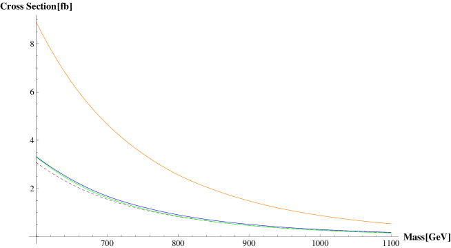
Figure 1: Pair production cross sections at the LHC as a function of heavy lepton mass: $pp\rightarrow\chi^{-}\chi^{+}$ (solid blue), $pp\rightarrow\chi^{0}\bar{\chi}^{0}$ (dashed brown), $pp\to\chi^{+}\chi^{0}$ (solid orange) and $pp\to\chi^{-}\bar{\chi}^{0}$ (solid green). The cross sections are given for a single heavy generation.

III.2 Signature

Most studies of heavy vector-like leptons assume no new Yukawa interaction, so that the neutral heavy leptons are stable. This improves the possibility of detection and allows for a variety of detection strategies Allanach:2001sd with an LHC mass reach of $\sim 1\;TeV$. In our case, however, the heavy leptons decay to SM leptons and electroweak gauge bosons or Higgs particles, leading to final states with multiple leptons and light jets. In the case of a light Higgs decaying predominantly into $b\bar{b}$ it is also possible to have heavy $b$ jets, otherwise the Higgs decays into pairs of electroweak gauge bosons allowing for many particles in the final state. Although the decay products described above seem complicated, the lack of final state neutrinos (except from $W$ and $Z$ decays) allows for a detection strategy based on reconstruction of the heavy lepton mass.

The process that we are looking at is

$$pp \to \chi^{+}\chi^{0},$$

$$\chi^{+}\to\ell_{1}^{+}Z^{0}/h^{0},\ \ \ Z^{0}/h^{0}\to{\rm jets},$$

$$\chi^{0}\to\ell_{2}^{\mp}W^{\pm},\ \ \ W^{\pm}\to\nu\ell_{3}^{\pm},$$

where $\ell$ stands for $e$ or $\mu$. The relevant diagram is shown in Fig. 2. The main signature that we are looking at is thus that of three isolated high $p_{T}$ leptons.

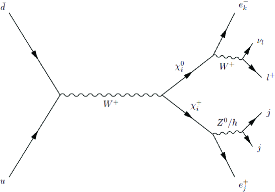
Figure 2: The leading heavy leptons pair-production process, and the decay modes that we use for detection.

The process

$$pp\to\chi^{0}\bar{\chi}^{0}\to W^{+}W^{-}\ell^{+}\ell^{-},$$ (11)

where one of the $W$-bosons decays leptonically and the other decays hadronically leads to the same final state, but it contributes at much lower rate.

III.3 Event selection

The final state we are considering has a clean signature of three isolated high $p_{T}$ leptons. Standard model processes with such a final state are rare; the dominant sources are $t\bar{t}$ pairs with an associated production of a $W/Z$ boson, as well as di-boson production, $WZ$ and $ZZ$. Since most of these processes involve a leptonic $Z$ decay, they can be efficiently suppressed by imposing a $Z$-veto, i.e. the requirement that no opposite-sign lepton pair is present in the event with invariant mass close to that of the $Z$ boson. We have also considered as possible backgrounds $Zb\bar{b}$ and di-lepton $t\bar{t}$, where additional leptons may be produced by the decay of $B$-mesons in the $b$-jets. All signal and background samples for this study were generated with MadGraph Alwall:2007st at $E_{\rm cm}=14$ TeV, with showering and hadronization done by PYTHIA Sjostrand:2006za , and detector effects simulated with the PGS fast simulation package pgs .

Fig. 3 shows the transverse momentum distributions of the reconstructed leptons and the two leading jets, for a signal sample with $m_{\chi}=500$ GeV.

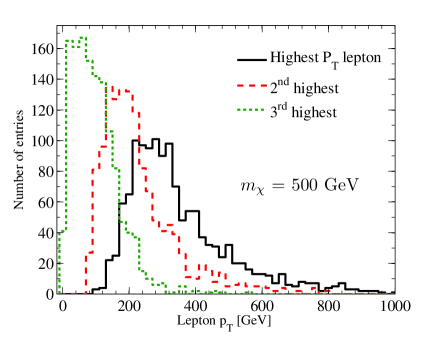
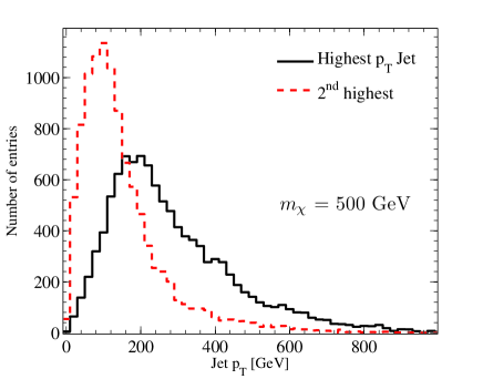
Figure 3: Distributions of transverse momenta in a signal sample corresponding to $m_{\chi}=500$ GeV for (a) the three final charged leptons, and (b) the two leading final jets.

Taking these distributions into consideration, we applied the following selection cuts:

1. Exactly three isolated leptons, not all same-sign, with $p_{T}>25$ GeV, of which at least two have $p_{T}>80$ GeV;

2. At least two jets with $p_{T}>25$ GeV or one jet with $p_{T}>50$ GeV;

3. The $Z$-veto is applied by requiring that $|m_{\ell^{+}\ell^{-}}-m_{Z}|>25$ GeV.

Isolation cuts for electrons were applied by the default PGS reconstruction algorithm. The isolation cuts for muons are defined as follows:

1. The summed transverse momentum in $\Delta R=0.4$ cone around the muon (excluding the muon itself) is $<5$ GeV;

2. The ratio of transverse energy in a grid of $3\times 3$ calorimeter cells around the muon (including the muons cell) to the transverse momentum of the muon is $<0.1$.

Table 2 presents the numbers of events passing the selection criteria (in fb). The signal corresponds to model LL, where there are three quasi-degenerate heavy leptons.

Table 2: Number of events corresponding to integrated luminosity of 1 fb^-1: total (first column); passing the selection criteria before imposing the $Z$ veto (second column); passing all cuts (third column). The last column reports the number of events that we generated for our simulation. The signal sample corresponds to three heavy lepton generations with $m_{\chi}=500$ GeV. It includes all production and decay modes (i.e. $\chi^{0}\bar{\chi}^{0},\chi^{+}\chi^{-},\chi^{\pm}\chi^{0}$), and the branching ratio refers to a three lepton final state. We use $m_{h}=120$ GeV.

Process	$W/Z$ Decay	$\sigma\times\mathcal{BR}$ [fb]	Selection [fb]	$Z$ veto [fb]	Generated events
$t\bar{t}Z$	$Z\to\ell^{+}\ell^{-}$	155.7	2.19	0.052	32.7K
$t\bar{t}W$	$3W\to 3(\ell\nu)$	13.95	0.174	0.139	23.7K
$ZZ$	$2Z\to 2(\ell^{+}\ell^{-})$	71.6	0.632	0.004	10K
$WZ$	$Z\to\ell^{+}\ell^{-}$, $W\to\ell\nu$	157	0.471	$<0.016$	10K
$t\bar{t}$	$2W\to 2(\ell\nu)$	33329	0.054	0.018	1.8M
$b\bar{b}Z$	$Z\to\ell^{+}\ell^{-}$	60000	0.027	$<0.027$	2.3M
Signal		19.0	12.8	12.0	25K

III.4 Reconstruction

Reconstruction of the heavy lepton mass requires the identification of the SM lepton originating from the $W$ decay. One possibility is immediately ruled out, since this lepton can only be one of the two leptons which have the same sign. We have calculated the transverse mass of the $W$ for both of those leptons:

$$(m_{T}^{W})^{2}=2p_{T}^{\ell}p_{T}^{\rm miss}(1-\cos\phi_{\ell,{\rm miss}}),$$ (12)

The distributions of $m_{T}^{W}$ are shown in Fig. 4, for the correct and for the wrong lepton assignments. The combination that yields the lower value was designated as the $W$ decay product. The correct lepton configuration was selected with this procedure at about 93% of the events.

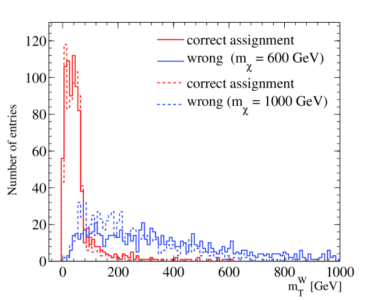
Figure 4: Distributions of the $W$ transverse mass with correct (red) and wrong (blue) lepton assignments, for heavy lepton masses of 600 (solid) and 1000 (dotted) GeV.

The two remaining opposite sign leptons, assumed to be produced directly by the heavy lepton-pair decays, were then assigned to the charged and neutral lepton decays according to their charges. Note that the above reconstruction procedure equally applies to events with a heavy neutral lepton pair and the same final state (11).

The transverse mass of the heavy neutral lepton was calculated according to

$$(m_{T}^{\chi^{0}})^{2}=m_{\ell^{+}\ell^{-}}^{2}+2(E_{T}^{\chi^{0}}p_{T}^{\rm miss}-{\bf p}_{T}^{\chi^{0}}\cdot{\bf p}_{T}^{\rm miss}),$$ (13)

where ${\bf p}_{T}^{\chi^{0}}={\bf p}_{T}^{\ell^{+}}+{\bf p}_{T}^{\ell^{-}}$, with $\ell^{+}$ and $\ell^{-}$ the two leptons associated with the $\chi^{0}\to W^{+}\ell^{-}\to\nu\ell^{+}\ell^{-}$ decay, and $E_{T}^{\chi^{0}}=\sqrt{m_{\ell^{+}\ell^{-}}^{2}+|{\bf p}_{T}^{\chi^{0}}|^{2}}$.

The invariant mass of the heavy charged lepton was reconstructed from the momenta of the two highest $p_{T}$ jets in the event and the lepton that has opposite charge to that of the $W$:

$$m_{\chi^{\pm}}^{2}=(p_{j1}+p_{j2}+p_{\ell})^{2}.$$ (14)

If the $Z/h$ is highly boosted, it can be reconstructed as a single jet. Therefore in the case that there is only a single reconstructed jet in the event with $p_{T}>50$ GeV, $p_{j2}$ is omitted from (14). The distributions of the reconstructed $m_{\chi^{\pm}}$ and $m_{T}^{\chi^{0}}$ are shown in Fig. 5, for $m_{\chi}=700$ GeV.

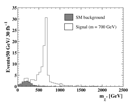
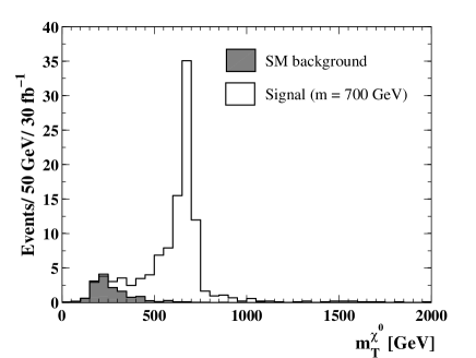
Figure 5: (a) Reconstructed invariant mass of the heavy charged lepton. (b) Reconstructed transverse mass of the neutral heavy lepton.

III.5 Obtaining flavor constraints

We focus here on model LL, which has three quasi-degenerate heavy leptons, each decaying to one of the light lepton flavors, $e,\mu,\tau$. Events are classified by the flavor of the two leptons associated with the heavy pair decay. We are interested in $N_{ij}$, the observed numbers of events in each flavor composition $\ell_{i}^{\pm}\ell_{j}^{\mp}$. The MLFV prediction is that

$$N_{ee} = N_{\mu\mu}=N_{\tau\tau},$$

$$N_{e\mu} = N_{e\tau}=N_{\mu\tau}=0.$$ (15)

Our analysis allows us to test two of these predictions, namely

$$N_{ee}=N_{\mu\mu},\ \ \ N_{e\mu}=0.$$ (16)

For the flavored cross section ratio estimates, we considered events within a window of 150 GeV around the mass peak of both $m_{\chi^{\pm}}$ and $m_{T}^{\chi^{0}}$. As is evident in Fig. 5, standard model background in this region is negligible. In Fig. 6, the reconstructed transverse mass $m_{T}^{\chi^{0}}$ is shown separately for the three different flavor compositions, $e^{+}e^{-}$, $\mu^{+}\mu^{-}$ and $e^{\pm}\mu^{\mp}$. Ideally, there should be no events in the $e\mu$ final state. In practice, however, a small number of the signal events are reconstructed as such, mostly due to misclassification of leptons in the event. Another possible source of contamination are $\tau$ pairs, decaying to $e$ and $\mu$, however this contribution was found to be negligible.

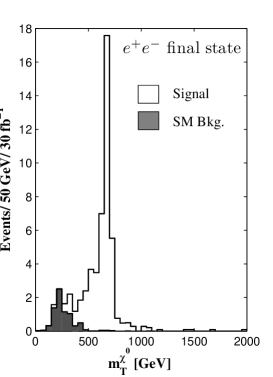
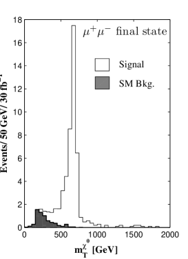
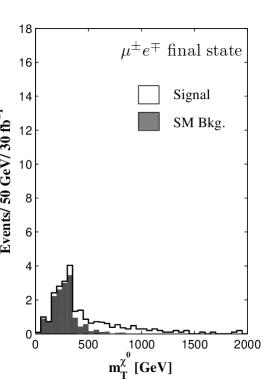
Figure 6: Number of events as a function of the reconstructed transverse mass $m_{T}^{0}$, for $m_{\chi}=700$ GeV and with an integrated luminosity of $30$ fb^-1, for the different flavor final states: (a) $ee$, (b) $\mu\mu$, and (c) $e\mu$.

To set limits on the ratios of different flavor final states we have treated the observed number of events of each category as independent Poisson variables. In such a case, the exact confidence intervals at a confidence level $1-\alpha$ are given by the following formula James:1980my :

$$B_{L,U} = A_{L,U}/(1-A_{L,U}),$$ (17)

$$A_{L} = F^{-1}(\alpha/2;n_{2},n_{1}+1),$$

$$A_{U} = F^{-1}(1-\alpha/2;n_{2}+1,n_{1}),$$

where $F(p;a,b)$ is the cumulative distribution function of a Beta distribution with parameters $a$ and $b$, at a value $p$, and $n_{1,2}$ are the observed numbers of events. $B_{L}$ and $B_{U}$ are the lower and upper bounds, respectively. The results are shown in Figs. 7 and 8. For the ratio $N_{e\mu}/(N_{ee}+N_{\mu\mu})$, the presence of small number of signal events in the $\mu^{\pm}e^{\mp}$ final state, due to misclassification, slightly weakens the obtained upper limit. This effect however is very small; to demonstrate this we also consider an “ideal” scenario in which the number of observed events $N_{e\mu}$ is set exactly to zero, as would be expected in our model in case of perfect reconstruction and no backgrounds. Those ideal limits are also shown in Fig. 8. For example, for a heavy lepton mass of $m_{\chi}=500$ GeV and with 30 fb^-1, the upper bound is only degraded due to backgrounds from approximately 0.02 to 0.03.

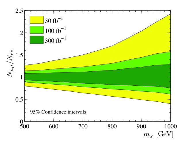
Figure 7: The power of the LHC experiments to constrain the ratio $N_{\mu^{+}\mu^{-}}/N_{e^{+}e^{-}}$ (for models where this ratio is unity) as a function of the heavy lepton mass. A value outside the colored area can be rejected at 95% CL for the corresponding integrated luminosity (dark green, light green, yellow for, respectively, 300, 100, 30 fb^-1).

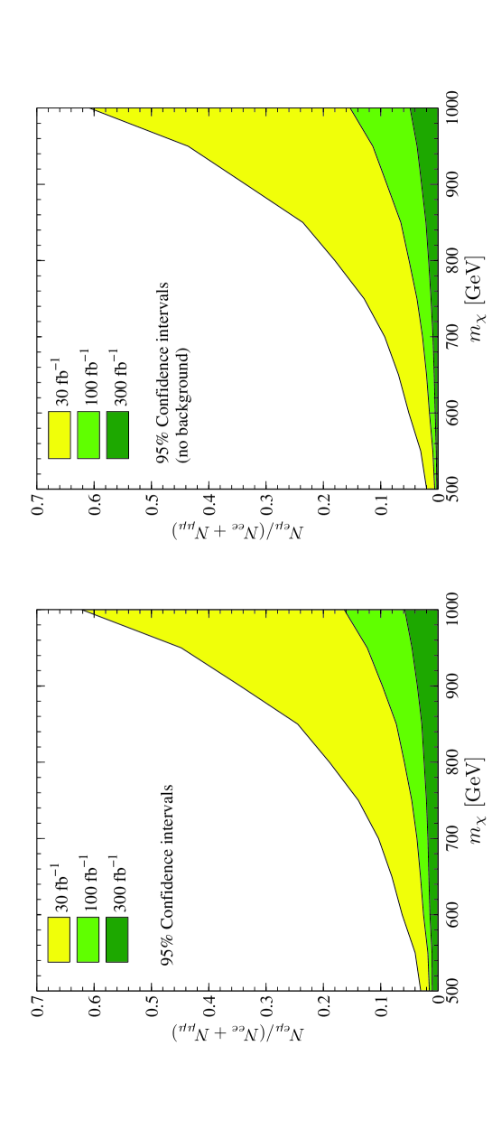
Figure 8: Right: The power of the LHC experiments to constrain the ratio $N_{e\mu}/(N_{ee}+N_{\mu\mu})$ (for models where this ratio is zero) as a function of the heavy lepton mass. A value above the colored region can be rejected at 95% CL for the corresponding integrated luminosity (dark green, light green, yellow for, respectively, 300, 100, 30 fb^-1). Left: similar limits for an ideal scenario in which there is no background, such that the uncertainty is purely statistical.

The obtained limits are given for the ratios of observed number of events. Within a realistic experimental environment one would have to take into account the different detection efficiencies of electrons vs. muons (which are approximately equal in PGS). The difference in energy resolution might also play a role. This effect is expected, however, to be very small, since the resolutions of the reconstructed masses ($m_{T}^{\chi^{0}}$ and $m_{\chi^{\pm}}$) are mostly driven by the energy resolution of jets. The ratio of reconstruction efficiencies of electrons vs. muons could be measured to a very high accuracy by comparing e.g. $Z\to e^{+}e^{-}$ to $Z\to\mu^{+}\mu^{-}$ events. With $\mathcal{O}(10^{5})$ such events expected per $1\;{\rm fb}^{-1}$, the attainable uncertainty of the efficiency ratio is expected to be negligible for our purposes. Thus, while a detailed study of such experimental effects is beyond the scope of this work, we expect the results presented here to be robust.

IV Implications for MLFV

The models presented in Section II.1 demonstrate that there could be a variety of mass spectra and couplings that are consistent with the principle of MLFV. In particular,

• The mass spectrum can be either quasi-degenerate or hierarchical. In the first case, we may have three heavy leptons within the reach of the LHC, in the latter only one.

• The couplings of the heavy vector-like leptons to the light, chiral ones can be either universal or hierarchical. While this has an effect on the lifetimes (which cannot be measured), it does not affect the overall number of events in each flavor.

There is, however, one feature that that is common to all our MLFV models:

• The couplings of the heavy vector-like leptons to the light, chiral ones are flavor-diagonal. In other words, we can describe the heavy lepton mass eigenstates as, approximately, heavy electron, muon and tau.

We are able to test the diagonality of the couplings in two independent ways, which are described in Section III.5. First, the comparison of the number of $e^{+}e^{-}$ events to the number of $\mu^{+}\mu^{-}$ events, where the MLFV prediction, for the case that both types of events are observed, is one. (The other possibility, in case of hierarchical spectrum, is that there are only $e^{+}e^{-}$ events.) As can be seen from Fig. 7, with 300 fb^-1 and $m_{\chi}\sim 500$ GeV, this prediction can be tested with an accuracy of order ten percent. With 30 fb^-1 and $m_{\chi}\sim$ TeV, this prediction can be tested to within a factor of 2.5.

Second, we can search for $e\mu$ events which, according to MLFV, should not be present. As can be seen from Fig. 8, with 300 fb^-1 and $m_{\chi}\sim 500$ GeV, the ratio between the flavor non-diagonal and flavor-diagonal events can be constrained to lie below the percent level. With 30 fb^-1 and $m_{\chi}\sim$ TeV, the bound is of order 0.6.

Low energy searches for flavor changing neutral current decays, such as $\mu\to e\gamma$, put strong constraints on the product of the mass splitting and the mixing angle between the heavy leptons. Regardless of the strength of such low energy constraints, ATLAS/CMS can provide flavor information that is not available from low energy data. In particular, the $e\mu$-test will constrain the mixing angle in the heavy sector for any finite mass splitting.

When ATLAS and CMS experiments collect enough data, they will also be able to understand in more detail their capabilities in identifying tau-leptons. It will become possible then to test also all tau-related predictions of Eq. (III.5). While the experimental accuracy of these measurements is expected to be poorer than the tests of Eq. (16), it may well be that violations of MLFV predictions are larger when tau-leptons are involved.

The analysis proposed in this paper will become much easier if, in addition to the charged heavy leptons, there exists a $Z^{\prime}$-boson that is light enough to be produced at the LHC and heavy enough to decay into a $\chi\bar{\chi}$ pair. Indeed, such a scenario, with stable heavy leptons, was described in Ref. Bauer:2009cc as a scenario that can be probed by a low energy and low luminosity initial LHC data set, and which is not ruled out by the Tevatron and other measurements. In such a case, we expect an ${\cal O}(16\pi^{2})$ enhancement in the number of signal events. It would mean that some informative (though rough) flavor measurements will be possible with as little as few hundreds of pb^-1 of integrated luminosity.

References

- (1) G. D’Ambrosio, G. F. Giudice, G. Isidori and A. Strumia, Nucl. Phys. B 645, 155 (2002) [arXiv:hep-ph/0207036];
- (2) L. J. Hall and L. Randall, Phys. Rev. Lett. 65, 2939 (1990);
- (3) R. S. Chivukula and H. Georgi, Phys. Lett. B 188, 99 (1987);
- (4) A. J. Buras, P. Gambino, M. Gorbahn, S. Jager and L. Silvestrini, Phys. Lett. B 500, 161 (2001) [arXiv:hep-ph/0007085];
- (5) A. L. Kagan, G. Perez, T. Volansky and J. Zupan, Phys. Rev. D 80, 076002 (2009) [arXiv:0903.1794 [hep-ph]].
- (6) V. Cirigliano, B. Grinstein, G. Isidori and M. B. Wise, Nucl. Phys. B 728, 121 (2005) [arXiv:hep-ph/0507001].
- (7) V. Cirigliano and B. Grinstein, Nucl. Phys. B 752, 18 (2006) [arXiv:hep-ph/0601111].
- (8) V. Cirigliano, G. Isidori and V. Porretti, Nucl. Phys. B 763, 228 (2007) [arXiv:hep-ph/0607068].
- (9) G. C. Branco, A. J. Buras, S. Jager, S. Uhlig and A. Weiler, JHEP 0709, 004 (2007) [arXiv:hep-ph/0609067].
- (10) M. C. Chen and H. B. Yu, Phys. Lett. B 672, 253 (2009) [arXiv:0804.2503 [hep-ph]].
- (11) B. C. Allanach, J. P. Conlon and C. G. Lester, Phys. Rev. D 77, 076006 (2008) [arXiv:0801.3666 [hep-ph]].
- (12) J. L. Feng, C. G. Lester, Y. Nir and Y. Shadmi, Phys. Rev. D 77, 076002 (2008) [arXiv:0712.0674 [hep-ph]].
- (13) J. L. Feng, S. T. French, C. G. Lester, Y. Nir and Y. Shadmi, Phys. Rev. D 80, 114004 (2009) [arXiv:0906.4215 [hep-ph]].
- (14) J. L. Feng et al., JHEP, in press [arXiv:0910.1618 [hep-ph]].
- (15) A. J. Buras, L. Calibbi and P. Paradisi, arXiv:0912.1309 [hep-ph].
- (16) M. I. Gresham and M. B. Wise, Phys. Rev. D 76, 075003 (2007) [arXiv:0706.0909 [hep-ph]].
- (17) Y. Grossman, Y. Nir, J. Thaler, T. Volansky and J. Zupan, Phys. Rev. D 76, 096006 (2007) [arXiv:0706.1845 [hep-ph]].
- (18) S. Dittmaier, G. Hiller, T. Plehn and M. Spannowsky, Phys. Rev. D 77, 115001 (2008) [arXiv:0708.0940 [hep-ph]].
- (19) G. Hiller and Y. Nir, JHEP 0803, 046 (2008) [arXiv:0802.0916 [hep-ph]].
- (20) C. P. Burgess, M. Trott and S. Zuberi, JHEP 0909, 082 (2009) [arXiv:0907.2696 [hep-ph]].
- (21) G. Hiller, J. S. Kim and H. Sedello, arXiv:0910.2124 [hep-ph].
- (22) J. M. Arnold, M. Pospelov, M. Trott and M. B. Wise, arXiv:0911.2225 [hep-ph].
- (23) M. E. Peskin and T. Takeuchi, Phys. Rev. D 46, 381 (1992).
- (24) J. Alwall et al., JHEP 0709, 028 (2007) [arXiv:0706.2334 [hep-ph]].
- (25) S. Kretzer, H. L. Lai, F. I. Olness and W. K. Tung, Phys. Rev. D 69, 114005 (2004) [arXiv:hep-ph/0307022].
- (26) T. Sjostrand, S. Mrenna and P. Z. Skands, JHEP 0605, 026 (2006) [arXiv:hep-ph/0603175].
- (27) http://www.physics.ucdavis.edu/ conway/research/software/pgs/pgs4-general.htm
- (28) B. C. Allanach, C. M. Harris, M. A. Parker, P. Richardson and B. R. Webber, JHEP 0108, 051 (2001) [arXiv:hep-ph/0108097].
- (29) J. A. Aguilar-Saavedra, Nucl. Phys. B 828, 289 (2010) [arXiv:0905.2221 [hep-ph]].
- (30) F. James and M. Roos, Nucl. Phys. B 172, 475 (1980).
- (31) C. W. Bauer, Z. Ligeti, M. Schmaltz, J. Thaler and D. G. E. Walker, arXiv:0909.5213 [hep-ph].