Fractional Vector Calculus and Fractional Special Function

Abstract

Fractional vector calculus is discussed in the spherical coordinate framework. A variation of the Legendre equation and fractional Bessel equation are solved by series expansion and numerically. Finally, we generalize the hypergeometric functions.

I Introduction

Fractional calculus is the calculus of differentiation and integration of non-integer orders podlubny ; kilbs . During last three decades, fractional calculus has gained much attention due to its demonstrated applications in various fields of science and engineering, such as anomalous diffusion scale , fractional dynamical systems B-vanderPol ; Brussel ; happiness , fractional quantum mechanics shroedinger , fractional statistics and thermodynamics entropy , to name a few.

Fractional vector calculus (FVC) is important in describing processes in fractal media, fractional electrodynamics and fractional hydrodynamics poisson ; fvc . But an effective FVC is still lacking. There are many problems in defining an effective FVC. One is that fractional integral and fractional derivative are defined “half” , that is to say, they are defined only on the right or the left side of an initial point. And if we make fractional series expansion, functions are all expanded on the right or the left neighborhood of the initial point. We cannot across this cutting point. So if we want to describe the behavior near the initial point, we need define both the right and the left functions. The situation will become even more complicated when we deal with high dimensions. In this letter we will define FVC in spherical coordinate framework. Since in the spherical coordinate framework the radius is naturally bounded to the positive half, we need just one fractional derivative.

Using this frame, we will discuss the Laplacian equation yzj with fractional radius derivative in 3-d space and the heat conduct equation yzj in 2-d space with cylindrical symmetry. As a result, the corresponding special functions will be generalized. Finally, we will generalize hypergeometric functions wzx ; wiki_HyperF ; wiki_ConfHyperF .

II Fractional calculus

To start, let’s briefly recall some basic facts in fractional calculus podlubny ; kilbs . There are many ways to define fractional integral and fractional derivative. In this letter we will use Riemann-Liouville fractional integral and Caputo fractional derivative.

Let $f(x)$ be a function defined on the right side of $a$. Let $\alpha$ be a positive real. The Riemann-Liouville fractional integral is defined by

$$I^{\alpha}f(x)=\frac{1}{\Gamma(\alpha)}\int_{a}^{x}(x-\xi)^{\alpha-1}f(\xi)~{}d\xi.$$ (1)

The integral has a memory kernel.

Let $A\equiv[\alpha]+1$. The Caputo fractional derivative is defined by

$$D^{\alpha}f(x) = I^{A-\alpha}\frac{d^{A}}{dx^{A}}f(x)$$ (2)

$$= \frac{1}{\Gamma(A-\alpha)}\int_{a}^{x}(x-\xi)^{A-\alpha-1}\frac{d^{A}}{d\xi^{A}}f(\xi)~{}d\xi.$$

They have the following properties:

$$D^{\alpha}(x-a)^{\beta}=0,~{}~{}~{}~{}~{}~{}~{}~{}~{}~{}~{}~{}~{}~{}~{}~{}~{}~{}~{}~{}~{}~{}~{}~{}\beta\in\{0,1,...,[\alpha]\};$$ (3)

$$D^{\alpha}(x-a)^{\beta}=\frac{\Gamma(\beta+1)}{\Gamma(\beta-\alpha+1)}(x-a)^{\beta-\alpha},\beta~{}\text{otherwise};$$ (4)

$$I^{\alpha}(x-a)^{\beta}=\frac{\Gamma(\beta+1)}{\Gamma(\beta+\alpha+1)}(x-a)^{\beta+\alpha}.~{}~{}~{}~{}~{}~{}~{}~{}~{}~{}~{}~{}~{}~{}~{}~{}~{}$$ (5)

These properties are just fractional generalizations of

$$\frac{d^{n}}{dx^{n}}x^{m}=\frac{m!}{(m-n)!}x^{m-n},~{}~{}~{}~{}n\in N,~{}~{}m\neq 0,$$ (6)

$$\int_{0}^{x}dx~{}x^{m}=\frac{m!}{(m+1)!}x^{m+1}.$$ (7)

For a ‘good’ function, one can define its fractional Taylor series

$$f(x)=\sum_{m=0}^{\infty}(D^{\alpha})^{m}f(x)\big{|}_{x=a}\cdot[(I^{\alpha})^{m}\cdot 1].$$ (8)

Explicitly,

$$(I^{\alpha})^{m}\cdot 1=\frac{1}{\Gamma(m\alpha+1)}(x-a)^{m\alpha}.$$ (9)

III Fractional vector calculus

As has been aforementioned, fractional derivative is defined only on the right or the left half of the real line, which gives complications in defining an effective FVC with Cartesian coordinates. So it may be more feasible to do FVC with spherical coordinates.

III.1 Spherical coordinates

The spherical coordinates of 3-dimension space is a triplet $(r,\theta,\phi)$. In one-order calculus, the gradient of a scale function $u(r,\theta,\phi)$ is

$$\textbf{Grad}~{}u=\bigg{(}\textbf{e}_{r}\frac{\partial}{\partial r}+\textbf{e}_{\theta}\frac{1}{r}\frac{\partial}{\partial\theta}+\textbf{e}_{\phi}\frac{1}{r\text{sin}\theta}\frac{\partial}{\partial\phi}\bigg{)}u.$$ (10)

We generalize this definition to fractional calculus as

$$\textbf{Grad}^{\alpha}~{}u=\bigg{(}\textbf{e}_{r}D^{\alpha}_{r}+\textbf{e}_{\theta}\frac{\Gamma(\alpha+1)}{r^{\alpha}}\frac{\partial}{\partial\theta}+\textbf{e}_{\phi}\frac{\Gamma(\alpha+1)}{r^{\alpha}\text{sin}^{\alpha}\theta}\frac{\partial}{\partial\phi}\bigg{)}u,$$ (11)

where $D^{\alpha}_{r}~{}u=\frac{1}{\Gamma(A-\alpha)}\int_{0}^{r}(r-\rho)^{A-\alpha-1}\frac{d^{A}}{d\rho^{A}}u(\rho,\theta,\phi)d\rho$. For anisotropic space, $\alpha$ is a function of $\theta$ and $\phi$. For isotropic space, $\alpha$ is a constant and independent of $\theta$ and $\phi$. We will just consider the isotropic case.

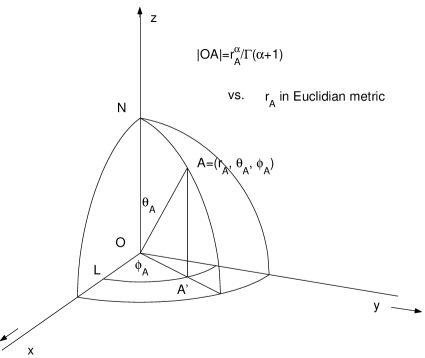
Figure 1: Spherical framework with fractional radius derivative. $|OA|=\frac{1}{\Gamma(\alpha+1)}r_{A}^{\alpha}$, $\widehat{NA}=\frac{1}{\Gamma(\alpha+1)}r_{A}^{\alpha}\theta_{A}$, and $\widehat{LA^{\prime}}=\frac{1}{\Gamma(\alpha+1)}r_{A}^{\alpha}\text{sin}^{\alpha}\theta_{A}~{}\phi_{A}$.

By this definition, the real space metric is changed to an effective metric. This can be easily seen from Fig. 1. The radius $|OA|$ now is $[I^{\alpha}_{r}\cdot 1]|_{r=0}^{r=r_{A}}=\frac{1}{\Gamma(\alpha+1)}r_{A}^{\alpha}$; the arc length $\widehat{NA}=\frac{1}{\Gamma(\alpha+1)}r_{A}^{\alpha}\theta_{A}$ and the arc length $\widehat{LA^{\prime}}=\frac{1}{\Gamma(\alpha+1)}r_{A}^{\alpha}\text{sin}^{\alpha}\theta_{A}~{}\phi_{A}$. This kind of metric is not addictive since $|OB|\neq|OA|+|AB|$ even when $O$, $A$ and $B$ are on the same straight line. This is due to the non-locality of the fractional operations.

By the above generalization, the divergence of a vector function $\textbf{A}=(A_{r},A_{\theta},A_{\phi})$ is

$$\text{div}^{\alpha}~{}\textbf{A}=\frac{1}{r^{2\alpha}\text{sin}^{\alpha}\theta}D^{\alpha}_{r}(r^{2\alpha}\text{sin}^{\alpha}\theta A_{r})+\frac{\Gamma(\alpha+1)}{r^{2\alpha}\text{sin}^{\alpha}\theta}\frac{\partial}{\partial\theta}(r^{\alpha}\text{sin}^{\alpha}\theta A_{\theta})+\frac{\Gamma(\alpha+1)}{r^{2\alpha}\text{sin}^{\alpha}\theta}\frac{\partial}{\partial\phi}(r^{\alpha}A_{\phi}).$$ (12)

The Laplacian of a scale function $u(r,\theta,\phi)$ will be

$$\triangle^{\alpha}~{}u \equiv \text{div}^{\alpha}\textbf{Grad}^{\alpha}~{}u$$ (13)

$$= \frac{1}{r^{2\alpha}}D^{\alpha}_{r}(r^{2\alpha}D^{\alpha}_{r}~{}u)+\frac{\Gamma^{2}(\alpha+1)}{r^{2\alpha}\text{sin}^{\alpha}\theta}\frac{\partial}{\partial\theta}(\text{sin}^{\alpha}\theta\frac{\partial}{\partial\theta}~{}u)+\frac{\Gamma^{2}(\alpha+1)}{r^{2\alpha}\text{sin}^{2\alpha}\theta}\frac{\partial^{2}}{\partial\phi^{2}}~{}u.$$

The rotor operator can be defined as well. Since in this letter we do not deal with the rotor, its definition will not be given.

III.2 Polor coordinates

Likewise, the fractional gradient operator of two dimensions in polor coordinates can be defined as

$$\textbf{Grad}^{\alpha}~{}u=\bigg{(}\textbf{e}_{r}D^{\alpha}_{r}+\textbf{e}_{\theta}\frac{\Gamma(\alpha+1)}{r^{\alpha}}\frac{\partial}{\partial\theta}\bigg{)}u.$$ (14)

The divergence is

$$\text{div}^{\alpha}~{}\textbf{A}=\frac{1}{r^{\alpha}}D^{\alpha}_{r}(r^{\alpha}A_{r})+\frac{\Gamma(\alpha+1)}{r^{\alpha}}\frac{\partial}{\partial\theta}A_{\theta}.$$ (15)

The Laplacian of a scale function $u(r,\theta)$ is

$$\triangle^{\alpha}~{}u \equiv \text{div}^{\alpha}\textbf{Grad}^{\alpha}~{}u$$ (16)

$$= \frac{1}{r^{\alpha}}D^{\alpha}_{r}(r^{\alpha}D^{\alpha}_{r}~{}u)+\frac{\Gamma^{2}(\alpha+1)}{r^{2\alpha}}\frac{\partial^{2}}{\partial\theta^{2}}u.$$

IV Fractional spherical equation and fractional cylindrical equation

In this section, we consider the Laplacian equation with the 3-d Laplacian operaror defined above and the fractional heat conduct equation in a 2-d space with cylindrical symmetry.

IV.1 Fractional Laplacian equation

With the Laplacian operator defined above, the Laplacian equation becomes

$$\triangle^{\alpha}~{}u=\frac{1}{r^{2\alpha}}D^{\alpha}_{r}(r^{2\alpha}D^{\alpha}_{r}~{}u)+\frac{\Gamma^{2}(\alpha+1)}{r^{2\alpha}\text{sin}^{\alpha}\theta}\frac{\partial}{\partial\theta}(\text{sin}^{\alpha}\theta\frac{\partial}{\partial\theta}~{}u)+\frac{\Gamma^{2}(\alpha+1)}{r^{2\alpha}\text{sin}^{2\alpha}\theta}\frac{\partial^{2}}{\partial\phi^{2}}~{}u=0.$$ (17)

This equation can be solved by separation of variables. Let $u=R(r)\Theta(\theta)\Phi(\phi)$ and substitute, the result is

$$\frac{1}{\Theta\text{sin}^{\alpha}\theta}\frac{d}{d\theta}\bigg{(}\text{sin}^{\alpha}\theta\frac{d\Theta}{d\theta}\bigg{)}+\frac{1}{\Phi\text{sin}^{2\alpha}\theta}\frac{d^{2}\Phi}{d\phi^{2}}=-\lambda,$$ (18)

$$\frac{1}{R}D^{\alpha}_{r}(r^{2\alpha}D^{\alpha}_{r}R)=\lambda\Gamma^{2}(\alpha+1).$$ (19)

The second equation can be solved by fractional series expansion. Let $R=\sum_{m=-\infty}^{\infty}c_{m}r^{m\alpha}$, and substitute, the result is that the nonzero components are the ones with $m$ satisfying

$$\frac{\Gamma(m\alpha+\alpha+1)}{\Gamma(m\alpha-\alpha+1)}=\lambda\Gamma^{2}(\alpha+1).$$ (20)

Otherwise, $c_{m}$=0.

The first equation is a variation of the ordinary spherical harmonic equation. By further decomposition, it turns to

$$\frac{d^{2}\Phi}{d\phi^{2}}+m^{2}\Phi=0,~{}~{}~{}~{}~{}(m=0,1,2,3,...)$$ (21)

$$\frac{\text{sin}^{\alpha}\theta}{\Theta}\frac{d}{d\theta}\bigg{(}\text{sin}^{\alpha}\theta\frac{d\Theta}{d\theta}\bigg{)}=m^{2}-\lambda\text{sin}^{2\alpha}\theta.$$ (22)

The first equation is simple. The second equation can be transformed by changing variables $x=\text{cos}\theta$ and $p(x)=\Theta(\theta)$ to

$$(1-x^{2})\frac{d^{2}p}{dx^{2}}-(1+\alpha)x\frac{dp}{dx}+\bigg{[}\lambda-\frac{m^{2}}{(1-x^{2})^{\alpha}}\bigg{]}p=0.$$ (23)

This is a variation of the ordinary associated Legendre equation yzj ; wzx . By setting $\alpha=1$, we recover the ordinary associated Legendre equation.

When $m=0$ it is the Legendre equation. Make the ansatz $p(x)=\sum_{n=0}^{\infty}c_{n}x^{n}$ and substitute, we find that the terms with even powers of $x$ and the terms with odd powers of $x$ are independent, so we can write $p(x)=c_{0}\cdot p_{\text{even}}(x)+c_{1}\cdot p_{\text{odd}}(x)$. The relation of successive coefficients is

$$c_{n+2}=c_{n}\frac{n^{2}+n\alpha-\lambda}{(n+2)(n+1)}.$$ (24)

Let $\alpha=1$ and $\lambda=l(l+1)$, we will get the Legendre polynomials. We calculated numerically the functions with some different values of the parameters and displayed the results in Fig. 2 and Fig. 3.

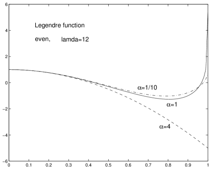
Figure 2: Legendre even function. Since the fractional index $\alpha$ occurs as a multiplicative factor in the variation version of the Legendre equation, small difference from 1 will not make large changes to the profile. We calculated the function with other small difference $\alpha$’s, but the results are not shown for their curves are very close to each other. Notice the direct of the curves.

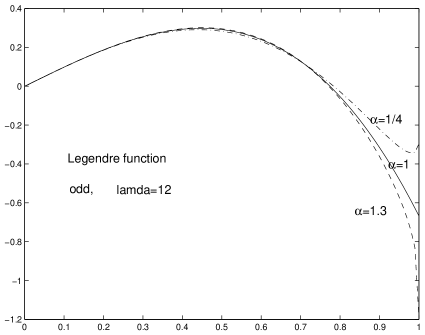
Figure 3: Legendre odd function. Notice the direct of the curves.

IV.2 Fractional cylindrical equation

The heat conduct equation in 2-d space is

$$\frac{\partial u}{\partial t}=a^{2}\triangle_{2}u.$$ (25)

Here $\triangle_{2}$ is the two dimensional Laplacian operator. Using the fractional cylindrical Laplacian operator defined above, this equation becomes

$$\frac{\partial u}{\partial t}=\frac{1}{r^{\alpha}}D^{\alpha}_{r}(r^{\alpha}D^{\alpha}_{r}~{}u)+\frac{\Gamma^{2}(\alpha+1)}{r^{2\alpha}}\frac{\partial^{2}}{\partial\theta^{2}}u.$$ (26)

By separation of variables $u(t,r,\theta)=R(r)\Theta(\theta)T(t)$, it can be decomposed to

$$T^{\prime}+a^{2}k^{2}T=0,$$ (27)

$$\frac{\partial^{2}\Theta}{\partial\theta^{2}}+\nu^{2}\Theta=0,$$ (28)

$$\frac{1}{\Gamma^{2}(\alpha+1)}r^{\alpha}D^{\alpha}_{r}(r^{\alpha}D^{\alpha}_{r}~{}R)+k^{2}\frac{r^{2\alpha}}{\Gamma^{2}(\alpha+1)}R-\nu^{2}R=0.$$ (29)

The first two equations are simple. The third equation is a fractional generalization of the Bessel equation yzj ; wzx . It can be solved by fractional series expansion. Since Bessel equation is singular at $r=0$. We must use such ansatz: $R=r^{\alpha\rho}\sum_{m=0}^{\infty}c_{m}r^{\alpha m}$. Substitute it into the above equation, we get

$$c_{0}\bigg{[}\bigg{(}\frac{\Gamma(\alpha\rho+1)}{\Gamma(\alpha\rho-\alpha+1)}\bigg{)}^{2}-\nu^{2}\Gamma^{2}(\alpha+1)\bigg{]}=0,$$ (30)

$$c_{1}\bigg{[}\bigg{(}\frac{\Gamma(\alpha\rho+\alpha+1)}{\Gamma(\alpha\rho+1)}\bigg{)}^{2}-\nu^{2}\Gamma^{2}(\alpha+1)\bigg{]}=0,$$ (31)

$$c_{m}\bigg{[}\bigg{(}\frac{\Gamma(\alpha\rho+\alpha m+1)}{\Gamma(\alpha\rho+\alpha m-\alpha+1)}\bigg{)}^{2}-\nu^{2}\Gamma^{2}(\alpha+1)\bigg{]}+c_{m-2}k^{2}=0.$$ (32)

To have a starting term, $c_{0}\neq 0$, so

$$\bigg{[}\bigg{(}\frac{\Gamma(\alpha\rho+1)}{\Gamma(\alpha\rho-\alpha+1)}\bigg{)}^{2}-\nu^{2}\Gamma^{2}(\alpha+1)\bigg{]}=0,$$ (33)

and $c_{1}=0$.

By the recursive relation, a solution is implied

$$R_{\rho}(r)=r^{\alpha\rho}\sum_{n=0}^{\infty}(-1)^{n}d_{n}k^{2n}r^{\alpha\cdot 2n},$$ (34)

where $d_{0}=1$,

$$d_{n}=d_{n-1}\frac{1}{\bigg{[}\bigg{(}\frac{\Gamma(\alpha\rho+\alpha\cdot 2n+1)}{\Gamma(\alpha\rho+\alpha\cdot 2n-\alpha+1)}\bigg{)}^{2}-\nu^{2}\Gamma^{2}(\alpha+1)\bigg{]}},$$ (35)

and $\rho$ satisfies Eq.(33).

Eq.(33) in one-order calculus ($\alpha=1$) is simply $\rho=\pm\nu$. We meshed in Fig. 4 the surface defined by the equation (33). After solving the equation with $\nu=3$ for $\rho$ when $\alpha$ varies, we plotted in Fig. 5 $R_{\rho}(r)$ belonging to different values of $\alpha$.

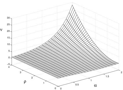
Figure 4: Parameters of fractional Bessel function. $\nu$ as a function of $\alpha$ and $\rho$.

Figure 5: Fractional Bessel function. The fractional index $\alpha$ shows up in the exponentials of the fractional Bessel series; a small difference from 1 changes the profile largely. For a big $\alpha$, $\rho$ is small, so the change is suppressed.

V Fractional hypergeometric function

There are other types of special functions in mathematical physics. A most famous one is the hypergeometric function wzx ; wiki_HyperF ; wiki_ConfHyperF . In this section, we will try to define a fractional generalization of the hypergeometric functions.

Let’s first consider the generalization of the confluent hypergeometric differential equation:

$$z^{\alpha}(D^{\alpha})^{2}y+(c-z^{\alpha})D^{\alpha}y-ay=0.$$ (36)

Here $a$ and $c$ are complex parameters. When $\alpha=1$, this is the ordinary confluent hypergeometric equation.

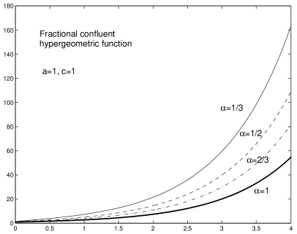
Figure 6: Fractional confluent hypergeometric function.

Introducing the fractional Taylor series

$$y(z)=\sum_{k=0}^{\infty}c_{k}z^{\alpha\cdot k},$$ (37)

and substituting, we get the ratio of successive coefficients

$$\frac{c_{k+1}\cdot\Gamma(k\alpha+\alpha+1)}{c_{k}\cdot\Gamma(k\alpha+1)} = \frac{a+\frac{\Gamma(k\alpha+1)}{\Gamma(k\alpha-\alpha+1)}}{c+\frac{\Gamma(k\alpha+1)}{\Gamma(k\alpha-\alpha+1)}},$$ (38)

$$\frac{c_{1}\cdot\Gamma(\alpha+1)}{c_{0}} = \frac{a}{c}.$$ (39)

Thus we get a solution of the above differential equation,

$$y(z)=\sum_{k=0}^{\infty}\frac{(a)^{\alpha}_{k}}{(c)^{\alpha}_{k}}\frac{1}{\Gamma(k\alpha+1)}z^{\alpha\cdot k}.$$ (40)

Here $(a)^{\alpha}_{k}$ is defined as

$$(a)^{\alpha}_{0} = 1,~{}~{}~{}~{}~{}(a)^{\alpha}_{1}=a,$$

$$(a)^{\alpha}_{k} = (a)^{\alpha}_{1}\bigg{(}a+\frac{\Gamma(\alpha+1)}{\Gamma(1)}\bigg{)}...\bigg{(}a+\frac{\Gamma(k\alpha-\alpha+1)}{\Gamma(k\alpha-2\alpha+1)}\bigg{)},$$ (41)

$$~{}~{}~{}~{}~{}~{}~{}~{}~{}~{}~{}~{}~{}~{}~{}~{}~{}~{}~{}~{}~{}~{}~{}~{}~{}~{}~{}~{}~{}~{}~{}~{}~{}~{}~{}~{}~{}~{}~{}~{}~{}~{}~{}~{}~{}~{}~{}k\geq 2.$$

This can be seen as a fractional generalization of the rising factorial

$$(a)_{k}=a(a+1)...(a+k-1).$$ (42)

And the series (40) can be seen as a fractional generalization the confluent hypergeometric function. If $\alpha=1$, it is exactly the confluent hypergeometric function. Profiles of this series (40) with different values of $\alpha$ are displayed in Fig. 6.

For the fractional Gauss hypergeometric function, consider the following series

$$y(z)=\sum_{k=0}^{\infty}\frac{(a)^{\alpha}_{k}(b)^{\alpha}_{k}}{(c)^{\alpha}_{k}}\frac{1}{\Gamma(k\alpha+1)}z^{\alpha\cdot k},$$ (43)

which reduces to the Gauss hypergeometric series when $\alpha=1$.

The ratio of successive coefficients is

$$\frac{c_{k+1}\cdot\Gamma(k\alpha+\alpha+1)}{c_{k}\cdot\Gamma(k\alpha+1)}=\frac{\bigg{(}a+\frac{\Gamma(k\alpha+1)}{\Gamma(k\alpha-\alpha+1)}\bigg{)}\bigg{(}b+\frac{\Gamma(k\alpha+1)}{\Gamma(k\alpha-\alpha+1)}\bigg{)}}{\bigg{(}c+\frac{\Gamma(k\alpha+1)}{\Gamma(k\alpha-\alpha+1)}\bigg{)}},$$ (44)

or

$$c_{k+1}\cdot c\frac{\Gamma(k\alpha+1)}{\Gamma(k\alpha-\alpha+1)}+c_{k+1}\cdot\frac{\Gamma(k\alpha+\alpha+1)}{\Gamma(k\alpha-\alpha+1)}$$ (45)

$$=c_{k}\cdot ab+c_{k}\cdot(a+b)\frac{\Gamma(k\alpha+1)}{\Gamma(k\alpha-\alpha+1)}+c_{k}\cdot\frac{\Gamma(k\alpha+1)}{\Gamma(k\alpha-\alpha+1)}\frac{\Gamma(k\alpha+1)}{\Gamma(k\alpha-\alpha+1)}.$$

Since

$$y(z)=\sum_{k=0}^{\infty}c_{k}z^{\alpha\cdot k},$$ (46)

$$z^{\alpha}D^{\alpha}y(z)=\sum_{k=1}^{\infty}c_{k}\frac{\Gamma(k\alpha+1)}{\Gamma(k\alpha-\alpha+1)}z^{\alpha\cdot k},$$ (47)

the equation (45) can be translated to a fractional differential equation

$$ab\cdot y(z)+(a+b)z^{\alpha}D^{\alpha}y(z)+z^{\alpha}D^{\alpha}\big{[}z^{\alpha}D^{\alpha}y(z)\big{]}$$

$$~{}~{}~{}~{}~{}~{}~{}~{}~{}~{}~{}~{}~{}~{}~{}~{}~{}~{}=c\cdot D^{\alpha}y(z)+z^{\alpha}(D^{\alpha})^{2}y(z).$$ (48)

When $\alpha=1$, this equation reduces to the ordinary Gauss hypergeometric equation. We draw curves of some example functions in Fig. 7.

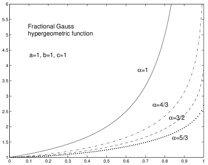
Figure 7: Fractional Gauss hypergeometric function. Gauss hypergeometric function is divergent at 1. From the figure we can see this is not the case for fractional equivalences with a bigger $\alpha$.

VI Summary

In this letter, we defined fractional vector calculus in the spherical coordinate framework. We discussed Laplacian equation and heat conduct equation in this kind of framework. Some special functions are generalized.

The geometry induced by fractional operations is non-addictive and nonlocal. This kind of geometry is not Riemannian; since fractional calculus has found applications in many areas of science and engineering, it is the effective geometry of such physics processes. It will be meaningful to investigate further this kind of geometry.

For a complete fractional vector calculus, fractional vector integral is indispensable. But in this letter we restrained ourselves from this direction. It will be interesting to discuss fractional vector integral in our framework and generalize Green’s, Stokes’ and Gauss’s theorem.

Special functions show up in different areas of physics and engineering. A fractional generalization of these functions may find applications in similar situations with anomalous tailing behaviors and/or nonlocal properties.

References

• (1) I. Podlubny, Fractional Differential Equations, Academic Press, San Diego, 1999.
• (2) A. A. Kilbas, H. M. Srivastava, J. J. Trujillo, Theory and Application of Fractional Differential Equations, Elsevier, Amsterdam, 2006.
• (3) G. M. Viswanathan, T. M. Viswanathan, arXiv:0807.1563v1 [physics.flu-dyn] 10 Jul 2008
• (4) V. Gariychuk, B. Datsko, V. Meleshko, Physica A 387 (2008) 418-424
• (5) V. Gariychuk, B. Datsko, Physics Letters A 372 (2008) 4902-4904
• (6) Lei Song, Shiyun Xu, Jianying Yang, Commun Nonlinear Sci Numer Simulat 15 (2010) 616-628
• (7) Nick Laskin, Phys. Rev. E 66, 056108 (2002)
• (8) Marcelo R. Ubriaco, Physics Letters A 373 (2009) 2516-2519
• (9) Sami I. Muslih, Om P.Agrawal, Int J Theor Phys, DOI: 10.1007/s10773-009-0200-1
• (10) Vasily E. Tarasov, Annals of Physics 323 (2008) 2756-2778
• (11) Zhenjun Yan, Mathematical Physics Equations, 2nd Edit., in Chinese, University of Science and Technology of China Press, Hefei, 2001.
• (12) Zhuxi Wang, Dunren Guo, Introduction to Special Functions, in Chinese, Peking University Press, Beijing, 2000.
• (13) http://en.wikipedia.org/wiki/Hypergeometric$\_$function
• (14) http://en.wikipedia.org/wiki/Confluent$\_$hypergeometric $\_$function