Magnetic interactions of substitutional Mn pairs in GaAs

Abstract

We employ a kinetic-exchange tight-binding model to calculate the magnetic interaction and anisotropy energies of a pair of substitutional Mn atoms in GaAs as a function of their separation distance and direction. We find that the most energetically stable configuration is usually one in which the spins are ferromagnetically aligned along the vector connecting the Mn atoms. The ferromagnetic configuration is characterized by a splitting of the topmost unoccupied acceptor levels, which is visible in scanning tunneling microscope studies when the pair is close to the surface and is strongly dependent on pair orientation. The largest acceptor splittings occur when the Mn pair is oriented along the $\langle 110\rangle$ symmetry direction, and the smallest when they are oriented along $\langle 100\rangle$. We show explicitly that the acceptor splitting is not simply related to the effective exchange interaction between the Mn local moments. The exchange interaction constant is instead more directly related to the width of the distribution of all impurity levels – occupied and unoccupied. When the Mn pair is at the (110) GaAs surface, both acceptor splitting and effective exchange interaction are very small except for the smallest possible Mn separation.

I Introduction

Experimental progress in the past 5 years has led to a large number of experimental studies of magnetic and nonmagnetic transition-metal impurities in semiconductors using advanced scanning tunneling microscope (STM) techniques.Yakunin et al. (2004, 2005); Kitchen et al. (2005, 2006, 2007); Garleff et al. (2008); Richardella et al. (2009) This effort was motivated in part by the hope that the high-resolution imaging and spatially resolved spectroscopic power of the STM could help in developing an accurate microscopic picture of dilute magnetic semiconductor (DMS) magnetism. In DMSs magnetic impurities provide local moments, which can couple to yield a collective ferromagnetic state. In the prototypical DMS, (Ga,Mn)As, the Mn impurities act as acceptors providing itinerant holes that can mediate long-range interactions between local moments. Among the open issues in DMS physicsDietl (2008) are the precise character of the hole states, the nature of the coupling of the holes with the local magnetic moments, and the properties of the ensuing magnetic interaction between local moments. STM experiments performed recentlyKitchen et al. (2006, 2007); Garleff et al. (2008); Richardella et al. (2009) are playing a decisive role in clarifying some of these issues.

In Ref. [Kitchen et al., 2006] STM substitution techniques were used to incorporate individual Mn atoms into Ga sites in a GaAs (110) surface. Real-space spectroscopic measurements in the vicinity of an isolated Mn impurity revealed the presence of a mid-gap resonance arising from a Mn induced acceptor state. High-resolution imaging showed that the acceptor wave function is strongly anisotropic with respect to the crystal axes of the host. When two Mn atoms were incorporated close to each other, two resonances appeared in the gap, split by approximately 0.5 eV. The splitting was found to be strongly dependent on the Mn pair orientation with respect to the GaAs crystal structure and on Mn separation. A simple toy model, describing acceptor states coupled to the Mn ion local moments of the two impurities,Schilfgaarde and Mryasov (2001) suggested that a measurable splitting of the acceptor levels could only occur if the two Mn local moments were ferromagnetically aligned.Kitchen et al. (2006) Since acceptor-level splitting is an observable indicator of ferromagnetic coupling, it seemed plausible that the dependence of this splitting on separation should be related at least qualitatively to the Mn-Mn exchange interaction. If so, the STM experiment could be used to measure exchange interactions between the Mn moments and test theories of this interaction. One of the purposes of the present study is to examine this relationship quantitatively.

Several of the experimental features uncovered in Ref. [Kitchen et al., 2006] could be qualitatively accounted for theoretically by a tight-binding model calculation for Mn in bulk GaAs presented in the same paper. A more thorough comparison between experiments and theoretical modeling, both for Mn atoms in the bulk and Mn near the surface is nevertheless necessary to interpret the experiments, motivating the present theoretical work. Here we consider a kinetic $p$-$d$ exchange tight-binding modelStrandberg et al. (2009) in which the effective exchange interaction between the hole states and the local Mn moments arises from hybridization of the impurity $d$ levels with $p$ levels of the host. The model is solved numerically for large super-clusters containing up to 3200 atoms. This approach allows us to place the Mn pair either in bulk GaAs or on the (110) surface.

Within this model, we study the electronic and magnetic properties of Mn pairs in GaAs, assuming that the two local magnetic moments are collinear, having either parallel [ferromagnetic (FM)] or antiparallel [antiferromagnetic (AFM)] relative orientation. One of our goals is to study the spin-orbit induced magnetic anisotropy energy of the system and see how this quantity is related to the properties of the mid-gap acceptor states. In the FM configuration the magnetic moment tends to point along the direction of the pair, while in the AFM configuration there is typically a quasi-easy plane perpendicular to the pair direction. As in the isolated Mn impurity case previously studied,Strandberg et al. (2009) we find that the sum of the individual anisotropy energies of the top two unoccupied valence band orbitals, mirrors the total anisotropy of the system. This shows that the picture of Mn-Mn interactions mediated by valence band holes is valid, and simplifies the interpretation of our numerical results. We then consider the properties of the acceptor levels for the two possible relative orientations of the Mn magnetic moments. In the FM configuration, which is generally found to be the ground state for most Mn pair orientations and Mn separations, the acceptor levels lie in a group just above the valence-band maximum and have a splitting that is enhanced by inter-ion hybridization. The group of six split levels can be viewed as a nascent version of the impurity band which forms in the bulk at small but finite Mn concentrations. In particular, the two unoccupied acceptor levels (i.e. occupied by holes), which fully determine both magnetic interaction and anisotropy energies have a finite splitting, which can be measured in experiment. For Mn pairs in bulk, we find that the acceptor splitting varies strongly with pair orientation and Mn separation, in agreement with experiment and previous calculations.Kitchen et al. (2006) The splitting is maximal for the most closely spaced Mn pair oriented along the $\langle 110\rangle$ direction, where it is of the order of few hundred meV, and very small for pairs oriented along $\langle 100\rangle$. For some Mn pairs, the wave functions of the two acceptor states have bonding and antibonding character, which is again consistent with experiment.Kitchen et al. (2006, 2007) These results support the validity of the kinetic $p$-$d$ exchange model.

In our study the energy difference between FM and AFM moment orientations is related to partial occupation of the acceptor impurity levels, which are split more widely in the FM configuration. When we calculate the exchange constant $J$ for the Mn-Mn interaction, as the difference between the ground-state energies of the two configurations, we find that $J$ is not in one-to-one correspondence with the splitting between the two unoccupied acceptor levels. In particular, the level splitting is much more anisotropic than $J$ with respect to the Mn pair orientation. On the other hand, we find that estimates of the width of the distribution of all impurity levels – occupied and unoccupied – are more directly related to $J$.

Effective exchange interactions between Mn ions in bulk (Ga,Mn)As have been calculated by several groups using either ab initio methods or more phenomenological approaches. Comparison of our results with other estimates is not always straightforward, since we have only two Mn moments and the exchange interactions are not strictly pairwise. The order of magnitude of our $J$ is nevertheless consistent with published results obtained from first-principles calculations, although values of $J$ for specific Mn pair directions and separations may differ. However, it is well-known that DMSs are not accurately described by the local-density-approximation often used in first principles methods. The discrepancies could either be due to the shortcomings of our model or to the inaccuracies of ab initio calculations.

We have also looked at how the Mn pairs interact when they are placed in a (110) GaAs surface. Typically, we find that the acceptor wave functions become highly localized at the surface and produce states that are deep in the band gap. As a result, the long-range interactions are much weaker and antiferromagnetic alignment of Mn spins is more likely to occur. The magnetic anisotropy energies at the surface are an order of magnitude smaller than in bulk, and tend to produce quasi-easy planes at close distances, reverting to isolated Mn anisotropy landscapes at larger separations. For Mn pairs in the (110) surface, the long-range behavior of the acceptor wave functions and acceptor splitting seems to agree less well with experiment than for Mn pairs in bulk GaAs. The tight-binding model that we use is of course less well justified when the Mn pair is in the surface. However, effects present in the experiment may contribute to this difference. In addition to an uncertainty in model parameters at the surface due to band-bending shifts of the acceptors, a large overlap with continuum states due to Zn co-dopants in the sample can cause a more extended, bulk-like Mn acceptor wave function. Beyond the scope of the present paper, care should also be taken in simulating the change in the effective potential experienced by surface electrons due to the addition and removal process introduced by the STM. Our results clearly demonstrate that modeling STM studies of the surface of a system as complicated as (Ga,Mn)As is highly nontrivial and requires additional work.

The paper is organized as follows. In Sec. II we review some theoretical aspects of the (Ga,Mn)As system and give a brief introduction to our tight-binding Hamiltonian. We also elaborate on a toy model that gives an idea of the system behavior expected when the Mn moments are parallel or antiparallel. The results for pairs of Mn along different symmetry directions in a fully periodic bulk-like environment are presented in Sec. III.1, and in Sec. III.2 for Mn pairs in the (110) GaAs surface. Finally, we summarize our conclusions in Sec. IV.

II Theory

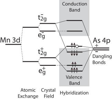
Figure 1: Schematic drawing of the level dynamics leading to a polarized acceptor at the top of the valence band. The Mn $3d^{5}$ up and down electrons are split by the atomic exchange in accordance with Hund’s first rule. The levels are further split by the crystal field into a doublet of $e_{g}$ and a triplet of $t_{2g}$-symmetry. The $t_{2g}$-levels hybridize with nearest neighbor dangling bond As $p$-states, such that the levels at the top of the valence band with spin parallel to the Mn spin are pushed up in energy. Spin up is denoted by + and spin down by -.

II.1 Hamiltonian for Mn impurities in GaAs

In this section we briefly review the basic physics of Mn impurities in GaAs, which motivates the choice of the tight-binding HamiltonianStrandberg et al. (2009) used throughout the paper. For more details the reader is referred to Ref. [Strandberg et al., 2009], where the same model was used to investigate the properties of individual Mn atoms in GaAs.

In the neutral state, consisting of the Mn²⁺ ion on a Ga site with a weakly bound hole, the Mn has spin $S=5/2$ and orbital moment $L=0$.Jungwirth et al. (2006) This is in accordance with Hund’s first rule that survives even when the Mn is embedded in the crystal. The Mn $3d^{5}$ electrons build up large, localized magnetic moments. Because the Mn is missing the Ga 4$p$ valence electron, it introduces a hole in the system, simultaneously acting as an acceptor and a source of magnetic moments. In bulk, the holes introduced by many Mn impurities form itinerant carriers that mediate the ferromagnetic coupling between localized moments. Fig. 1 shows a schematic drawing of what happens when a Mn substitutes a Ga in the GaAs lattice.Zhao et al. (2004) The Mn $3d^{5}$ up states (for example) that lodge in the valence band are exchange-split from the down states that end up in the conduction band. The crystal field imposes the tetrahedral host symmetry, resulting in a further split into a doublet of $e_{g}$ symmetry and a triplet of $t_{2g}$ symmetry.Vogl and Baranowski (1985) The $e_{g}$ states couple only weakly to the host. The $t_{2g}$ states on the other hand, hybridize with the As nearest neighbor dangling-bond $p$ states at the top of the valence band, forming bonding and antibonding combinations. Effectively, the neighboring As $p$ spins at the top of the valence band that are parallel to the Mn spin are shifted up in energy, whereas $p$ spins that are antiparallel to the Mn spin are shifted down. Therefore, the main effect of a single substitutional Mn with spin up, is to introduce three spin-polarized (”up”) levels above the top of the valence band and three spin-polarized (”down”) levels below. These six states are predominantly of As $p$ character. The hole introduced by a single Mn will occupy the highest of the three antibonding states (indicated by the empty circle in Fig. 1). In this way, the hybridization mechanism gives rise to an antiferromagnetic coupling between itinerant and localized spins by what is known as Zener’s kinetic-exchange mechanism.Zener (1951); Dietl et al. (2000); Bhattacharjee et al. (1983); Okabayashi et al. (1998) We account for this $p$-$d$ indirect exchange by introducing a classical Mn vector of magnitude 5/2, which couples to the neighboring As $p$ states. There are no explicit $d$ electrons in our model; they are accounted for only implicitly via the exchange interaction between the localized moments and the As $p$ spins on neighboring sites.

Our tight-binding kinetic exchange Hamiltonian takes the following form:

$$H =\sum_{ij,\mu\mu^{\prime},\sigma}t_{\mu\mu^{\prime}}^{ij}a_{i\mu\sigma}^{{\dagger}}a_{j\mu^{\prime}\sigma}^{\phantom{{\dagger}}}+J_{pd}\sum_{m}\sum_{n[m]}\vec{S}_{n}\cdot\hat{\Omega}_{m}$$

$$+\sum_{i,\mu\mu^{\prime},\sigma\sigma^{\prime}}\lambda_{i}\langle\mu,\sigma|\vec{L}\cdot\vec{S}|\mu^{\prime},\sigma^{\prime}\rangle a_{i\mu\sigma}^{{\dagger}}a_{i\mu^{\prime}\sigma^{\prime}}^{\phantom{{\dagger}}}$$

$$+\frac{e^{2}}{4\pi\varepsilon_{0}\varepsilon_{r}}\sum_{m}\sum_{i\mu\sigma}\frac{a_{i\mu\sigma}^{{\dagger}}a_{i\mu\sigma}^{\phantom{{\dagger}}}}{|\vec{r}_{i}\mathbf{-}\vec{R}_{m}|}+V_{\mathrm{corr}}.$$ (1)

The first term reproduces the band-structure of bulk GaAsChadi (1977) and contains the near-neighbor hopping and on-site energies in terms of the Slater-Koster parametersSlater and Koster (1954); Papaconstantopoulos and Mehl (2003) $t_{\mu\mu^{\prime}}^{ij}$ for the $s$ and $p$ electrons of Ga and As. In (1) $i$ and $j$ are atomic indices, $\mu$ and $\mu^{\prime}$ are orbital indices and $\sigma$ denotes spin. In simulating the (110) surface, buckling is accounted for by rescalingChadi (1978, 1979) the tight-binding parameters and modifying the direction cosines appropriately.

The second term implements the $p$-$d$ exchange mechanism described above. It couples the unit spin vector of Mn atom $m$: $\hat{\Omega}_{m}$, to the $p$ orbitals of the nearest neighbor As atoms $n[m]$: $\vec{S}_{n}=\tfrac{1}{2}~{}\sum_{\pi\sigma\sigma^{\prime}}a_{n\pi\sigma}^{{\dagger}}\vec{\tau}_{\sigma\sigma^{\prime}}a_{n\pi\sigma^{\prime}}$, where $\vec{\tau}$ is a vector of Pauli matrices. The value of $J_{pd}$ has been inferred by theoryTimm and MacDonald (2005) and experimentOhno (1998) to approximately $J_{pd}=1.5$ eV. The three $p$-$d$ hybridized levels, spin-polarized in the direction of the Mn moment $\hat{\Omega}_{m}$ are split from the three levels polarized in the opposite direction by an energy of order $J_{pd}$.

The third term in Eq. (1) accounts for SO interactions in an atomic approximation with the renormalized spin-orbit splittingsChadi (1977) $\lambda_{\text{Ga}}=2\lambda_{\text{Mn}}=58$ meV and $\lambda_{\text{As}}=140$ meV. Spin-orbit interaction causes the band energy to depend not only on the relative angles between different Mn spin directions, but also on spin-orientations relative to the lattice.

The fourth term of the Hamiltonian accounts for a long-range repulsive Coulomb interaction in the presence of a Mn impurity, which attracts a weakly bound hole and repels electrons. At the surface, we crudely account for the weaker dielectric screening by reducing the bulk dielectric constant $\varepsilon_{r}$ in half. The Coulomb behavior at short distances is parametrized in $V_{\mathrm{corr}},$ which is a Mn central cell correction term used as a parameter to tune the Mn acceptor level to the experimental position.Schairer and Schmidt (1974); Lee and Anderson (1964); Chapman and Hutchinson (1967); Linnarsson et al. (1997) It contains an on-site $V_{\mathrm{on}}=1.0$ eV (that is, acting on the Mn) and an off-site term $V_{\mathrm{off}}=2.4$ eV. The off-site Coulomb correction affects the nearest neighbor As atoms and together with $J_{pd}$ controls the amount of $p$-$d$ hybridization in the system and the range of the acceptor wave function.

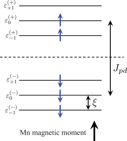
Figure 2: The six spin-polarized levels resulting from the $p$-$d$ hybridization around a Mn impurity, shown in Fig. 1. The three levels with orbital index $\mu=-1,0,+1$ above the valence band edge, polarized in the direction of the Mn moment, are higher in energy than the three corresponding levels polarized in the opposite direction by an amount of the order of the effective exchange constant $J_{pd}$. Spin-orbit interactions (and surface effects when present) lift the orbital degeneracy of the like-spin levels and cause a small admixture of opposite spin character. The topmost up-spin level is the acceptor level introduced by the Mn.

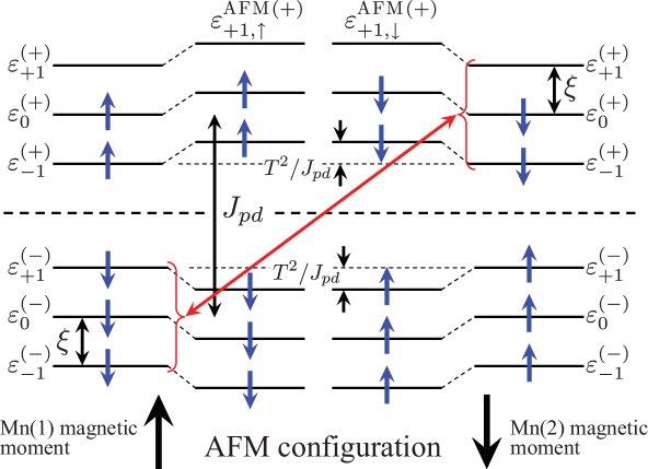
Figure 3: Toy model for two Mn atoms when the two local moments are aligned antiparallel – the AFM configuration. Each Mn site has six exchange-split itinerant levels that hybridize with the like-spin levels at the other Mn site. Note that like-spin levels have different energies at the two sites. The resulting hybridized levels, drawn in the middle, have their energy lowered or raised by $\sim T^{2}/J_{pd}$ where $T$ is the intersite hopping energy scale. This results in a net gain in energy because of the two holes introduced by the two Mn ions.

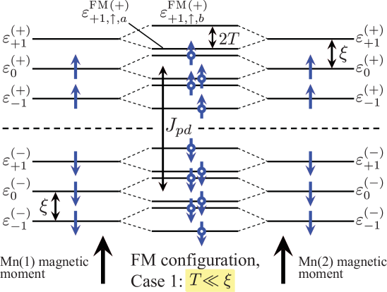
Figure 4: Toy model for two Mn atoms when the two local moments are aligned parallel – the FM configuration. Each Mn has six exchange-split itinerant levels that hybridize with the like-spin levels at the other Mn via hopping. Now, like-spin levels at the two sites are degenerate and give rise to bonding and antibonding states split by the hopping parameter $2T$ which causes a “widening of the band”. The resulting hybridized levels are drawn for the case when the hopping parameter $T$ is smaller than the spin-orbit induced splitting $\xi$. Note that for the acceptor (hole) states above the valence band edge, we use the convention of calling “bonding” the state with the higher energy (subscript $b=$ bonding and $a=$ antibonding).

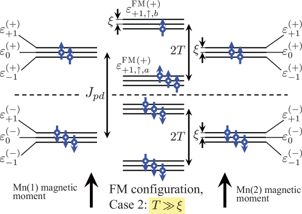
Figure 5: The same FM alignment of Mn spins as in Fig. 4, but for the case when the hopping parameter $T$ is much larger than the spin-orbit induced splitting $\xi$. The resulting impurity bandendnote50, of bandwidth $\approx 2T$, is partially filled when two holes are present, resulting in a large energy gain with respect to the uncoupled $T=0$ system.

II.2 Toy model for Mn pairs in GaAs

In this section we discuss a system of two Mn atoms in GaAs by means of a simple toy modelSchilfgaarde and Mryasov (2001) that elucidates the basic mechanism responsible for the effective coupling between their localized spins. The properties of this simple model will be very useful in interpreting the results of our numerical calculations in Sec. III.

For each Mn impurity in GaAs we will focus on the six spin-polarized levels at the top of the valence band, emerging from the $p$-$d$ hybridization shown in Fig. 1. These six levels are shown explicitly in Fig. 2 for one particular orientation of the Mn moment. The three levels above the valence-band edge with orbital angular momentum projection $\mu=0,\pm 1$, are spin-polarized in the direction of the Mn magnetic moment. Similarly, the corresponding three levels below the valence band edge are polarized in the opposite direction. Spin-orbit coupling (and surface effects when the Mn is not in the bulk) lifts the orbital degeneracy of the like-spin states. We model this splitting by introducing the energies

$$\varepsilon_{\mu}^{(\pm)}=\pm J_{pd}/2+\mu\xi\;,\qquad\mu=0,\pm 1\,$$ (2)

where $\xi$ represents the SO-induced splitting. Here $(+)$ and $(-)$ stand for the levels above and below the valence-band edge, respectively. Note that $\varepsilon_{\mu}^{(+)}-\varepsilon_{\mu}^{(-)}=J_{pd}$, where $J_{pd}$ is the effective exchange coupling used in Eq. (1). In the presence of spin-orbit interaction the spin is no longer a good quantum number, but we will assume that these states still have a predominant spin character, which is the same as when SO interaction is absent.

When two Mn impurities are present and close to each other, the system can lower the total energy by allowing hopping between two single-particle states with the same spin, each centered around one of the two Mn. Two different situations arise depending on whether the relative orientation of the two Mn moments is parallel or antiparallel. We assume that each state $|i,\mu,\sigma\rangle$, with $\sigma=\uparrow,\downarrow$ at Mn site $i$ will be coupled to the corresponding same spin state $|j,\mu,\sigma\rangle$ at the other Mn site $j$ by an effective hopping parameter $T_{\mu}$, which we take to be spin-independent. The single-particle Hamiltonian representing these two sets of itinerant spins coupled to the Mn local moment with hopping between sites is given by

$$H_{AFM}^{FM}=\sum_{\mu} \Big{(}\varepsilon_{\mu}^{(+)}c_{1\mu\uparrow}^{{\dagger}}c_{1\mu\uparrow}^{\phantom{{\dagger}}}+\varepsilon_{\mu}^{(-)}c_{1\mu\downarrow}^{{\dagger}}c_{1\mu\downarrow}^{\phantom{{\dagger}}}$$

$$+\varepsilon_{\mu}^{(\pm)}c_{2\mu\uparrow}^{{\dagger}}c_{2\mu\uparrow}^{\phantom{{\dagger}}}+\varepsilon_{\mu}^{(\mp)}c_{2\mu\downarrow}^{{\dagger}}c_{2\mu\downarrow}^{\phantom{{\dagger}}}\Big{)}$$

$$-\sum_{i\neq j,\sigma}T_{\mu}c_{i\mu\sigma}^{{\dagger}}c_{j\mu\sigma}{\phantom{{\dagger}}},$$ (3)

where the upper signs in superscript refer to the FM and the lower signs to the AFM configuration. The Hamiltonian in Eq. (3) corresponds to the Anderson-Hasegawa HamiltonianAnderson and Hasegawa (1955) with the angle $\theta$ between the spins equal to 0 and $\pi$, for the parallel and antiparallel configurations respectively.

The Hamiltonian is immediately diagonalized by noting that the spin and orbital characters are good quantum numbers. The nature of the resulting hybridized levels will depend on the relative orientation of the two Mn moments: in the FM configuration the two sets of unperturbed equal-spin states (one at each Mn site) are degenerate and will form bonding and antibonding combinations via hopping. By contrast, in the AFM configuration like-spins at different Mn sites have different energies and the hybridization will be reduced by a factor $\approx T_{\mu}/J_{pd}$.

In the AFM configuration the spectrum is doubly degenerate with energies

$$\varepsilon_{\mu\uparrow}^{\mathrm{AFM}(\pm)}=\varepsilon_{\mu\downarrow}^{\mathrm{AFM}(\pm)}=\mu\,\xi\pm\sqrt{T_{\mu}^{2}+J_{pd}^{2}/4}.$$ (4)

Fig. 3 shows a schematic view of the energy levels for the AFM configuration with a constant $T_{\mu}=T$. In the presence of holes, the total energy of the AFM state, $E_{\mathrm{tot}}^{\mathrm{AFM}}$, obtained by summing the energies of the occupied states, is lower than for the non-hybridized ($T_{\mu}=0$) state. The maximum gain occurs for the “half-filled” system consisting of six holes. For the case of two Mn introducing two holes (shown in Fig. 3), the energy gain of the AFM configuration is approximately $2T^{2}/J_{pd}$. This phenomenon is similar to the superexchange mechanism – arising within a one-band Hubbard model at half filling – which favors antiferromagnetic alignment of the itinerant spins on neighboring sites. Note that there are no $d$ electrons present in our model and that the superexchange between the local moments is brought about by the kinetic exchange between the itinerant spins. When the two Mn atoms are close to each other, oppositely aligned Mn spins allow the wave functions to spread out, thus lowering their kinetic energy by hopping.

In the FM configuration the spectrum is nondegenerate

$$\varepsilon_{\mu\uparrow b}^{\mathrm{FM}(+)}=\varepsilon_{\mu}^{(+)}+T_{\mu}\;,\quad\varepsilon_{\mu\uparrow a}^{\mathrm{FM}(+)}=\varepsilon_{\mu}^{(+)}-T_{\mu}\;,$$ (5)

$$\varepsilon_{\mu\downarrow a}^{\mathrm{FM}(-)}=\varepsilon_{\mu}^{(-)}+T_{\mu}\;,\quad\varepsilon_{\mu\downarrow b}^{\mathrm{FM}(-)}=\varepsilon_{\mu}^{(-)}-T_{\mu}\;,$$ (6)

where $\varepsilon_{\mu(\uparrow,\downarrow)b}^{\mathrm{FM}}$ and $\varepsilon_{\mu(\uparrow,\downarrow)a}^{\mathrm{FM}}$ are bonding and antibonding states respectively. The acceptor (hole) states are more bound when they are further away from the valence band top, which is the start of the continuum for hole states. Out of the two acceptor states arising from the hybridization of the degenerate like-spin states of energy $\varepsilon_{\mu}^{(+)}$, we therefore assign the label “bonding” to the one that occurs at higher energy, while the one with lower energy is denoted as “antibonding” [see Eq. 5].

The energy spectrum for the FM configuration is shown in Fig. 4 when the hopping parameter is smaller than the SO splitting, $T_{\mu}\equiv T\ll\xi$. The six$\frac{{}}{{}}$ acceptor levels above the valence band edge form an “impurity band”endnote50 with an associated bandwidth that increases with the splitting $T$. Note that for $T\ll\xi$, when two holes are present the total energy $E_{\mathrm{tot}}^{\mathrm{FM}}$ is the same as for the non-hybridized case, $T=0$. An energy gain equal to $-T$ occurs only when an odd number of holes are present. The opposite limit of a large hopping parameter, $T_{\mu}\equiv T\gg\xi$, is shown in Fig. 5. Since only two thirds of the “impurity band” is filled there is a net energy gain $\xi-2T$ due to the level splitting, which can stabilize the FM configuration against the AFM one. This mechanism that couples the itinerant spins ferromagnetically, corresponds to double exchange between the two sites. For a partially occupied impurity band the FM alignment tends to be energetically more favorable than the AFM when the widening of the band induced by hopping is large. The difference between the total energies of the two configurations defines an effective exchange constant $J\equiv(E_{\mathrm{tot}}^{\mathrm{AFM}}-E_{\mathrm{tot}}^{\mathrm{FM}})/2$ representing a Heisenberg-like magnetic interaction, $\mathcal{H}\propto-J\vec{S}_{\text{Mn}(1)}\cdot\vec{S}_{\text{Mn}(1)}$, between the local moments at the two Mn sites.

The actual hopping paths are of course more complicated than the ones shown in Figs. 3-5. In particular, for a hopping parameter $T_{\mu}$ depending strongly on the orbital character $\mu$, we expect the resulting FM configuration to be intermediate between the limiting cases of Fig. 4 and Fig. 5. In any case, the toy model predicts that the FM configuration will always be characterized by a splitting $\Delta_{\mathrm{acc}}$ of the two acceptor states, related either to covalency between individual acceptor levels or to spin-orbit coupling. The splitting is noticeably absent in the AFM configuration, where the two acceptor states are quasi-degenerate, and is therefore a landmark of the FM state. As mentioned in the introduction, the STM experiments do measure a significant splitting between the two acceptor states, which is a strong indication that the Mn pair is coupled ferromagnetically. It is therefore important to investigate if some kind of relationship exists between $\Delta_{\mathrm{acc}}$ and $J$. This can be the case if, for example, the level structure of the FM configuration is of the type sketched in Fig. 6. Here a dominating hopping term $T_{\mu=+1}$ gives rise to both a partially filled impurity bandendnote50 stabilizing the FM state, and a large acceptor splitting $\Delta_{\mathrm{acc}}=T_{\mu=+1}-T_{\mu=0}+\xi$, which will also be approximately related to the exchange energy gained by the FM configuration. As we will see later (following the discussion of Fig. 10), this is the case that best describes the numerical results of the microscopic Hamiltonian in Eq. (1).

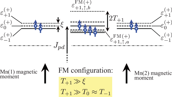
Figure 6: Toy model for two Mn sites in the FM configuration when one hopping matrix element ($T_{\mu=+1}$) is much larger than the other two and larger than the spin-orbit induced splitting $\xi$. Only the impurity levels above the valence-band edge are drawn. The half-occupied impurity band favors a FM alignment over the AFM configuration and the non-hybridized ($T_{\mu}=0$) system. The acceptor splitting is large and equal to $T_{\mu=+1}-T_{\mu=0}+\xi$. As we will see later (following the discussion of Fig. 10), this is the case that best describes the numerical results of the microscopic Hamiltonian in Eq. (1).

In the next Section we examine the properties of the six impurity levels when the Mn spins are parallel or antiparallel, and see how these states relate to the effective exchange constant $J$ and the magnetic anisotropy energy. Note that the trace of the $p$-$d$ exchange operator, summed over all valence band states is zero. If the impurity levels involve negligible conduction band character, it follows that the sum of the energies of all valence band states is independent of Mn spin orientations. Strandberg et al. (2009) Because of this property, exchange and interaction energies are expected to be accurately expressed in terms of the energies of the two empty valence band states.

In the evaluation of $J$, we will also approximate the total energy for the FM and AFM configurations by summing up the energies of the two unoccupied acceptor levels, or alternatively of the four topmost occupied levels. These results are compared the $J$ obtained by the difference between AFM and FM total energies. We will also consider other measures of the acceptor level structure broadening in Mn dimers, which might be more closely related to exchange interaction than the splitting of the top two levels. These measures include the splitting between the mean of the four occupied and the mean of the two unoccupied levels, and the effective ”bandwidth” of the six levels as obtained by calculating the standard deviation from their mean value.

III Results

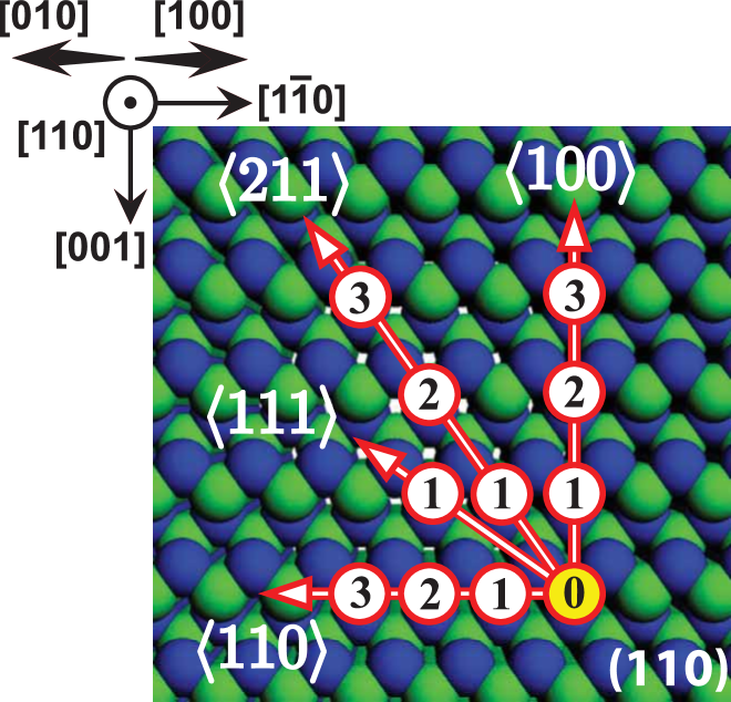
Figure 7: (Color online) Directions and separations of a Mn pair on the (110) surface. The two Mn atoms, replacing Ga atoms (bright green spheres), are marked 0 (first Mn atom) and 1,2,3 (second Mn atom) in correspondence with Fig. 8 below. Note that all equivalent symmetry directions $\langle...\rangle$ have been chosen in direct coordinates $[...]$, such that all the Mn pairs appear in the $\left(110\right)$ plane.

III.1 Mn-Mn interactions in bulk GaAs

In this section we study numerically the properties of substitutional Mn pairs in bulk GaAs. As shown in Fig. 7, we consider Mn pairs oriented along different crystalline directions at various separations. The two Mn are embedded in a 3200 atom GaAs supercell with periodic boundary conditions in all directions, corresponding to a Mn fraction of 0.06%. We consider collinear magnetic configurations in which the Mn moments are either parallel or antiparallel.

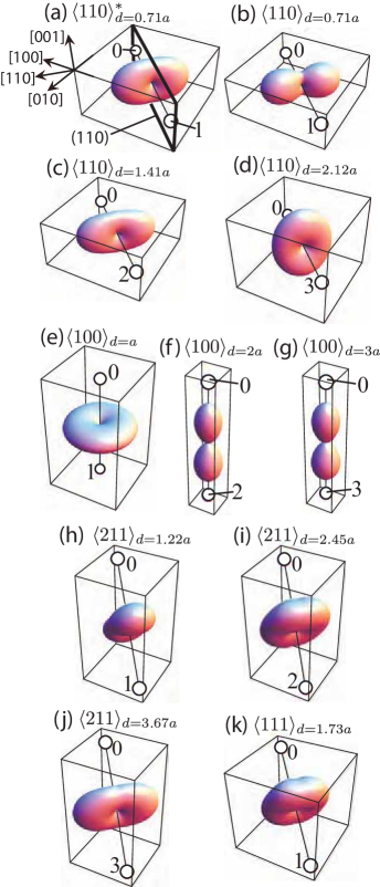
Figure 8: (Color online) Magnetic anisotropy in collinear variation of parallel Mn spins on the unit sphere. Generally, an easy axis is found to be parallel to the connecting Mn line, with the exception of the $\langle 100\rangle_{d=2a,3a}$. The $\langle 110\rangle^{\ast}$ shows the effect of non-additive Coulomb correction on the common As neighbor, yielding larger anisotropy barriers. In panel (a) the crystal axes have been marked and the same labels apply to all other panels. Also indicated is the (110) plane that contains all Mn pairs. The Mn are numbered in accordance with Fig. 7. The AFM configurations all have a higher total energy and the variations are inverted with respect to the FM ones.

III.1.1 Magnetic anisotropy energy

We begin by looking at the magnetic anisotropy of the system, which is defined as the dependence of the total ground-state energy $E_{\mathrm{tot}}(\hat{\Omega})$ on the direction of the Mn-pair magnetic moment, $\hat{\Omega}$. For the AFM configuration, $\hat{\Omega}$ is the direction of the staggered moment. Graphical representations of the magnetic anisotropy landscapes $E_{\mathrm{tot}}(\hat{\Omega})$ on the unit sphere of the all possible directions for $\hat{\Omega}$, are presented in Fig. 8 for the FM configurations. Each panel (a)-(k) refers to a Mn pair with a particular separation and orientation in the crystal, according to the notation defined in Fig. 7.

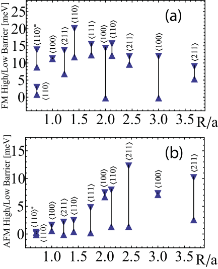
Figure 9: High and Low magnetic anisotropy barriers. In these graphs, zero corresponds to the minimum energy on the unit sphere. The anisotropy increases when the Coulomb correction is taken to be non-additive for $\langle 110\rangle^{\ast}$ in the FM configuration (a). The $\langle 110\rangle_{d=1.41}$ shows enhanced anisotropy barriers, with strong interactions along this symmetry direction. $\langle 100\rangle$ has a single barrier for the closest distance, but exhibits quasi-easy-planes (low barrier is zero) perpendicular to the connecting Mn line for longer distances. In the AFM configurations (b), the anisotropies gradually increase with distance as cancellations between the two acceptor levels decrease.

In these figures, what we actually plot is

$$E_{\mathrm{anis}}(\hat{\Omega})\equiv E_{\mathrm{tot}}(\hat{\Omega})-E_{\mathrm{tot}}^{\mathrm{min}},$$ (7)

as a function of the magnetic moment direction $\hat{\Omega}$. Each point of the “anisotropy surface” is obtained by measuring the ”distance” $\big{(}E_{\mathrm{tot}}(\hat{\Omega})-E_{\mathrm{tot}}^{\mathrm{min}}\big{)}$ from the center of the reference parallelepiped defined by the cubic axes $[100]$, $[010]$, and $[001]$. The center of the parallelepiped is also taken to be the center of the unit sphere of directions. Here $E_{\mathrm{tot}}^{\mathrm{min}}$ is the minimum value of $E_{\mathrm{tot}}(\hat{\Omega})$ upon varying $\hat{\Omega}$ that occurs along one of the easy directions. The actual values of the high and the low energy barriers of these systems are shown in Fig. 9. In the FM configurations, the bistable easy directions are generally found to be parallel to Mn pair axis. The two exceptions are the quasieasy planes perpendicular to the connecting line, formed when the Mn are spaced at two and three lattice constants along $\langle 100\rangle$ [see Fig. 8 (f) and (g)]. For these two configurations, the magnetic hard direction has 12-15 meV higher energy. The qualitatively different landscapes signal that the interactions along the $\langle 100\rangle$ direction differ from the other crystalline directions. For the shortest separation along $\langle 100\rangle$, $d=a=5.65~{}$A, a bistable easy axis parallel to the Mn-connecting line with a blocking barrier of around 11 meV is found. This means that a level crossing at the Fermi level occurs when the distance is increased from one to two lattice constants. Associated with this crossing is a change in the orbital character of the acceptors that results in a qualitatively different anisotropy.

Focusing now on the $\langle 110\rangle$ [with the Mn pair along $[1\bar{1}0]$, see Fig. 8 (b)-(d)], for which closely spaced As and Ga provide more direct hopping paths between the Mn, we see that there is a low barrier along the [001] axis and a high barrier along [110]. At the closest spacing, $d=0.7a$, the anisotropy energy is very small with barriers of 1-3 meV [see Fig. 8 (b)]. This configuration is special, because the off-site Coulomb correction on the common nearest neighbor As between the Mn is additive, giving it a large on-site energy that reduces anisotropy. The $\langle 110\rangle^{\ast}$ pair in Fig. 8 (a) shows the effect of a non-additive Coulomb correction on the common As neighbor, where the low and high barriers have increased to 9 and 14 meV. As we let the Mn move apart one step further along the $\langle 110\rangle$ with distance $d=1.4a,$ the high barrier attains the maximum value of all considered configurations of 21 meV, and a low barrier of 12 meV. At the longest considered separation along $\langle 110\rangle$, the low and high barriers are now 12 and 16 meV, respectively. The $\langle 211\rangle$ Mn pairs follow a similar evolution of the high and low barrier, relative the connecting Mn line, now with a low barrier along the [110] direction that changes to the high barrier with increasing distance. Distances are longer than for the $\langle 110\rangle$ pairs and therefore hybridization is weaker and the anisotropy energies drops by a few meV. At the larger separations along $\langle 211\rangle$ the bistable minima are tilted away from the connecting line, an indication that the single Mn anisotropy is becoming comparable to the Mn-Mn interaction energy. Even with a supercell of 3200 atoms we cannot exclude possible finite-size-effect contributions to the anisotropies. Nevertheless, we can get a good estimate of the barriers separating the generally bistable minima. The magnetic anisotropy in (Ga,Mn)As nanostructures, such as (Ga, Mn)As epilayers, is presently a topic of great interest.

Understanding the microscopic mechanisms of magnetic anisotropy in DMS is crucial in order be able to manipulate the magnetization vector by magnetic and electric fields.Chiba et al. (2009) For a review of recent theoretical and experimental works on magnetic anisotropy in (Ga, Mn)As see Ref. [Zemen et al., 2009], where ferromagnetic samples with a relatively high Mn content of a few percent are examined. Comparison with our results, which instead pertain to the magnetic anisotropy of isolated Mn dimers, is not straightforward. Our results could on the other hand be directly compared with those of STM experiments using a spin-polarized magnetic tipWiesendanger (2009) and an external magnetic field.

As we show below, all the AFM pairs have a higher total energy, which is expected on the basis of the heuristic toy model considerations. The AFM anisotropy landscapes are qualitatively inverted with respect to the FM ones, i.e., the bistable minima along the Mn dimer axis in the FM variation are replaced by quasieasy planes perpendicular to the dimer axis in the AFM variation. This inversion of hard and easy directions between FM and AFM can be understood by considering the FM configuration in the easy direction, where the spin-orbit splitting between the highest occupied and the lowest unoccupied levels is large, resulting in a lower total energy. In the corresponding AFM configuration, the two levels are of opposing spin character, such that the splitting is smaller and the total energy instead higher. In Fig. 9 (b), we see that the closer the Mn are, the smaller the anisotropy energies tend to be. This figure gives us an idea of the range of strongly interacting Mn. Weaker interactions at larger distances in the AFM configuration tends to increase the anisotropy, as the effectively spin-polarized region in the lattice around each Mn increases.

III.1.2 Character of acceptors for Mn pairs in bulk GaAs

The anisotropy of the embedded Mn dimers is accurately reflected in the anisotropy of the two acceptor levels and their associated wave functions. In this section we therefore perform a detailed analysis of various properties of the acceptor levels, such as their splitting and LDOS - quantities that are directly accessible by STM spectroscopy.

From now on we use the convention to denote with $\varepsilon_{-3}\;,\varepsilon_{-2}\;,\varepsilon_{-1}\;,\varepsilon_{0}$ the energies of four highest occupied states, while $\varepsilon_{1}$ and $\varepsilon_{2}$ denote the energies of the two acceptor levels. When mixing with the conduction band is negligible, the anisotropy energy landscape can be extracted from the the two acceptor levels using

$$E_{\mathrm{anis}}(\hat{\Omega})=-\sum_{i=1}^{2}[\varepsilon_{i}(\hat{\Omega})-\varepsilon_{i}^{\mathrm{min}}],$$ (8)

where $E_{\mathrm{anis}}(\hat{\Omega})$ is defined in Eq. (7) and the upper limit in the sum can be generalized to a greater number of acceptor levels. Equation (8) follows from the fact that the trace of the $p$-$d$ exchange operator in Eq. (1) summed over all valence band states including the acceptors is zero. In the FM variation of the Mn spins, the high-energy acceptor level, $\varepsilon_{2}(\hat{\Omega})$, varies very little and in a qualitatively opposite manner to the low-energy acceptor, $\varepsilon_{1}(\hat{\Omega})$. Its effect is therefore to reduce the much higher anisotropy coming from the lower acceptor level. In the AFM configuration small acceptor level variations partially cancel to a low total anisotropy below 1.5 lattice constants, and add up to a larger total anisotropy above this value.

SO interaction mixes spin components, such that the eigenstates are no longer of definite spin character. As a result, the acceptor states above the valence band edge, which without SO coupling have the same spin character as the corresponding localized Mn moment (”spin-up”), acquire a small component in the opposite direction (“spin-down”). In the FM cases, this results in a small spin down character of the acceptor levels, that increases with Mn distance primarily for the low acceptor, as it moves closer to the valence band. In the AFM variations, the two acceptor levels are now very close in energy and their spin character can vary by a large amount on the unit sphere due to spin-orbit interaction.

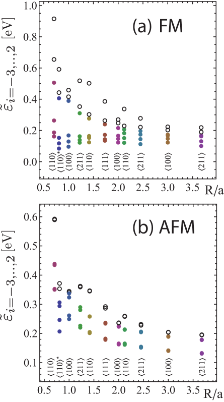
Figure 10: The four highest occupied (filled circles) and the two lowest unoccupied (empty circles) eigenstates as obtained by taking the spherical average. In the FM configuration (a) the splitting between the three upper and lower impurity levels decreases with distance, but the split between the two acceptor levels follows a more complex pattern, depending on pair orientation. In the AFM configuration (b) levels bunch up but are still split from each other by weaker hybridization. The $\langle 110\rangle^{\ast}$ has been shifted slightly to the right in order not to obscure the graph.

In Fig. 10 we plot the energies of the four highest occupied and the two unoccupied acceptor levels for all studied configurations. We consider spherical averages of these six energies over all possible moment directions, denoted by $\tilde{\varepsilon}_{i}\;,i=-3\;,\dots\;,2$.

In the FM configuration [Fig. 10 (a)] we find that there is a clear splitting between the three lowest and highest levels, in agreement with the results of the toy model shown in Fig. 5. The fact that three highest levels are also spread over a sizable energy range indicates that, at least for the shortest Mn separation, we are in the regime described by Fig. 6 of the toy model. Note in particular the large splitting of the two acceptor levels, as expected for aligned Mn spins. The level splitting and the overall width of the impurity bandendnote50 decreases with increasing Mn separation. Note also the strong dependence of the acceptor splitting on the orientation of the Mn pair. In particular, the FM acceptor splittings tend to be largest along the $\langle 110\rangle$ direction. It is also clear that the $\langle 100\rangle$ Mn pair behaves differently. Even if the splitting is large between the three lower and three upper levels, the splitting of the two acceptor levels is consistently smaller than for the other orientations.

In the AFM configuration the structure of the six energy levels is quite different and its salient features are nicely captured by the toy model result of Fig. 3. The levels are always essentially doubly degenerate; the splitting between doublets can be large for the shortest Mn separation and but it decreases quickly with distance and becomes of the order of the expected SO-induced splitting. In contrast to the FM case, there is no visible splitting between the acceptor levels. The only exception is the special case of the $\langle 110\rangle$ for the shortest Mn separation, where the six impurity levels abruptly drop down towards the valence continuum as the off-site Coulomb correction on the common As neighbor is decreased. Finally note that the $\langle 100\rangle$ pair sticks out with a more dense set of levels also in the AFM configuration

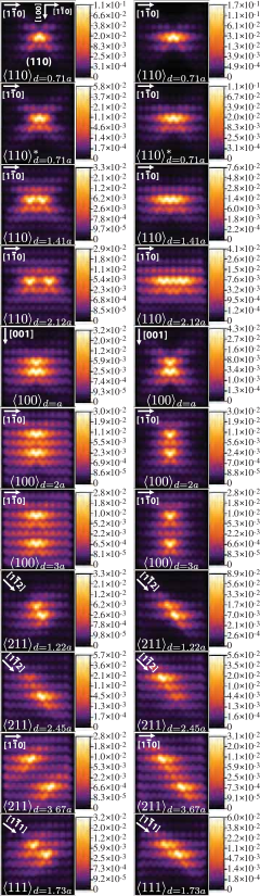
Figure 11: (Color online) LDOS of the lower-energy (left column) and the higher-energy (right column) acceptor level in the easy direction (indicated by white arrow in top left corners) for the FM configurations. Each row corresponds to a given crystal orientation and separation for of the Mn pair.

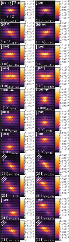
Figure 12: (Color online) LDOS of the lower-energy (left column) and the higher-energy (right column) acceptor level in the easy direction for the AFM configurations.

We proceed to discuss the Local Density Of States (LDOS) of the two acceptor levels - a property that can be probed by STM spectroscopy.Kitchen et al. (2006, 2007); Garleff et al. (2008); Richardella et al. (2009) Plots of the LDOS of the two acceptor levels in the (110) plane containing the two Mn, are shown in Fig. 11 for the FM and in Fig. 12 for the AFM configurations. The LDOS plots are generated from the tight-binding model calculations as in Refs. [Strandberg et al., 2009; Tang and Flatté, 2004]. In these plots the Mn spins are pointing in the magnetic easy directions, indicated by the arrow in the top left corner of each panel. The left column in each figure shows the LDOS of the lower energy acceptor state, which is closer to the valence band maximum; the right column refers to the acceptor with higher energy.

We first consider the $\langle 110\rangle$ pairs in the FM configuration (see Fig. 11). For the special case where the Mn atoms are separated by a common nearest neighbor As, the results change significantly depending on whether the off-site Coulomb correction is additive ($\langle 110\rangle_{d=0.71a}$) or non-additive ($\langle 110\rangle_{d=0.71a}^{\ast}$). We see that the effect of a non-additive Coulomb correction on the common As is to delocalize the acceptor wave functions. A more delocalized wave function generates larger anisotropy energies, as shown in Fig. 9. At the shortest Mn separation, both acceptor wave functions have bonding character, with the maximum spectral weight on the common As neighbor located between them. This situation is captured by the toy model, where the large hybridization occurring at small Mn separation gives rise to the level structure shown in Figs. 5 and 6, with both acceptors being of the bonding type. As the Mn ions move apart along $\langle 110\rangle$, the lower acceptor state develops more antibonding character with a significant decrease of the spectral weight between the two Mn sites, whereas the upper acceptor remains in a bonding-like state. Within our toy model, this implies that the two acceptor states correspond to bonding and antibonding states arising from the hybridization of degenerate levels in energy, spin and orbital character, as shown in Fig. 4.

In agreement with our results, the STM experiments for the $\langle 110\rangle$ pair find clear evidence that the two Mn-induced acceptor states have bonding and antibonding character, with the bonding state occurring at higher energies. Kitchen et al. (2006, 2007) An antibonding character for the lower energy state is observed experimentally also for the Mn pair with the shortest separation.Kitchen et al. (2007) While this does not seem to be case in our bulk $\langle 110\rangle_{d=0.71a}$ calculations (both states being essentially “bonding”), we do find that the value of the maximum LDOS on the As in between the Mn’s is around twice as large for the upper acceptor wave function.

For the $\langle 100\rangle$ pairs the upper acceptor exhibits a more localized signature, whereas the lower acceptor is more extended because it is closer to the valence continuum. Bonding and antibonding formations cannot be clearly seen, indicating that the hybridization between the two holes is much weaker along the $\langle 100\rangle$. This conclusion is also supported by the very small acceptor-energy splitting, as shown in Fig. 21. In the remaining directions $\langle 211\rangle$ and $\langle 111\rangle$ (rows 8-11), bonding and antibonding characters are visible, with more and less spectral weight in the region between the Mn, respectively.

In the AFM LDOS (see Fig. 12) there are no bonding or antibonding patterns for the two acceptor states, in agreement with the results of the toy model. Rather, a spatially symmetric separation seems to occur for some of the Mn pairs, in particular for larger distances along the $\langle 100\rangle$, $\langle 211\rangle$ and $\langle 111\rangle$ directions. For these pairs the upper and lower acceptor acquire opposite and rather definite spin characters in the easy direction. In this case spin up is located on one site and spin down on the other, whereas for $\langle 110\rangle$ the two acceptors are of mixed spin character.

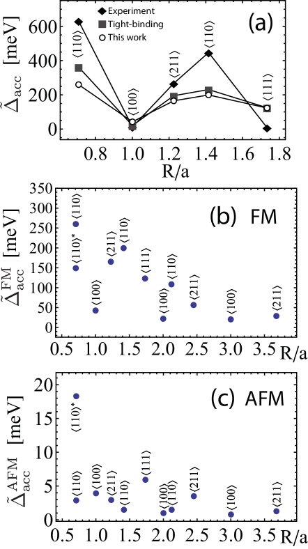
Figure 13: Acceptor level splittings as a function of pair orientation and distance. (a) shows a comparative plot of current and theoretical and experimental results from Ref. [Kitchen et al., 2006]. In (b) and (c) the FM and AFM results for all considered pairs are shown.

III.1.3 Acceptor splitting vs. effective exchange constant $J$

In this Section we take a closer look at the acceptor energy splitting $\Delta_{\mathrm{acc}}(\hat{\Omega})\equiv\varepsilon_{2}-\varepsilon_{1}$, focusing in particular on its spherical average $\tilde{\Delta}_{\mathrm{acc}}=\tilde{\varepsilon}_{2}-\tilde{\varepsilon}_{1}$. We will also compute the effective exchange constant $J(\hat{\Omega})$ and see if a relationship can be found between these two important quantities.

Fig. 13 shows the average acceptor splitting $\tilde{\Delta}_{\mathrm{acc}}$ in the FM and AFM configurations compared to the experimental and theoretical values reported in Ref. [Kitchen et al., 2006, 2007]. Our calculated splittings match the previous calculationsKitchen et al. (2006, 2007), and follow the trend of the measured splittings at the (110) surface. Fig. 13 (b) reveals that the splitting is largest for Mn pairs along $\langle 110\rangle$ directions, and very small for $\langle 100\rangle$ Mn pairs. The $\langle 211\rangle$ and $\langle 111\rangle$ Mn pairs exhibit smaller splittings than $\langle 110\rangle$, which has more direct hopping paths. Notice that there is some correlation between the splittings and the high barriers in Fig. 9 (a); higher anisotropy barriers correspond to a larger splitting.

Fig. 13 (a) shows that our tight-binding model as well as a previous theoryKitchen et al. (2006) based on a similar approach, systematically underestimates the acceptor splitting measured experimentally. This discrepancy could be due to inherent limited accuracy of the tight-binding method. However, it is also quite possible that part of the splitting seen experimentally is of Coulombic origin arising when electrons tunnel into the two different acceptor levels. In Fig. 13 (c) we see that the AFM splittings are very small compared to the FM ones, and are typically of the order of a few meV. As already noted above, the only exception is the $\langle 110\rangle^{\ast}$ pair. Reducing the Coulomb parameter on the common As neighbor dramatically lowers the acceptor energies [see Fig. 10 (b)], produces more extended wave functions (see Fig. 12), and increases mixing with valence band states.

We can now consider the effective exchange energy defined as $J(\hat{\Omega})=[E_{\mathrm{tot}}^{AFM}(\hat{\Omega})-E_{\mathrm{tot}}^{FM}(\hat{\Omega})]/[2\cdot(5/2)^{2}]$, where the factors of $5/2$ from the Mn spin magnitudes is absorbed in $J$. A positive (negative) $J$ implies that the Mn-Mn interactions are FM (AFM). As a result of the spin-orbit interaction, $J(\hat{\Omega})$ is an anisotropic quantity, that is, it depends on $\hat{\Omega}$.

Figure 14: Effective exchange couplings. A ferromagnetic coupling is always favored as all spherical averages $\tilde{J}>0$.

The effective $\tilde{J}$ as obtained by taking the spherical averages is shown in Fig. 14, where it can be seen that the FM configuration is always the most stable one, $\tilde{J}>0$. Only for separations greater than two lattice constants, do the SO-induced fluctuations in $J$ become comparable to the average value. Even then, ferromagnetism is always favored. The maximal value of $J$ generally occurs when the Mn spins are pointing along the pair axis.

The comparison between the acceptor splitting $\tilde{\Delta}_{\mathrm{acc}}^{\mathrm{FM}}$ for the FM state [Fig. 13 (b)] and the exchange constant $\tilde{J}$ [Fig. 14 (a)] shows that both quantities decay rapidly with Mn separation. However, there are noticeable differences between them, out of which two are most obvious. First of all, the relative value of $\tilde{J}$ for the $\langle 110\rangle_{d=0.71a}$ pair compared to all the other values is much larger than the corresponding value of $\tilde{\Delta}_{\mathrm{acc}}^{\mathrm{FM}}$. Secondly, $\tilde{\Delta}_{\mathrm{acc}}^{\mathrm{FM}}$ displays a much less monotonic decrease with Mn separation than $\tilde{J}$. In particular, the large dip for the $\langle 100\rangle_{d=a,2a}$ pairs is totally absent in the plot for $\tilde{J}$. A similar dip for the $\langle 100\rangle_{d=2a}$ pair is hinted but much less pronounced in the $\tilde{J}$ plot.

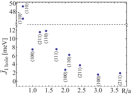
Figure 15: Effective exchange couplings for a system with two Mn and one hole. Adding one electron to the system, gives an effective exchange that is related to the acceptor splittings.

At this point it is useful to consider other quantities that can shed light on the relationship between the effective exchange interaction and the acceptor levels. We first consider the effective exchange constant for a Mn pair when only one hole is present or, equivalently, when the lower acceptor is occupied by an electron. The toy model results in Figs. 3 and 4 can help intuition and justify the rational of this choice: when an extra electron is added to these electronic configurations, only the topmost acceptor level is unoccupied in the FM state. In this case the acceptor splitting should be directly related to the energy gain stabilizing a FM state over the AFM state. The effect of occupying the lowest acceptor is shown in Fig. 15, where we plot $\tilde{J}_{\mathrm{1hole}}\equiv[\tilde{E}_{\mathrm{tot,1hole}}^{\mathrm{AFM}}-\tilde{E}_{\mathrm{tot,1hole}}^{\mathrm{FM}}]/[2\cdot(5/2)^{2}]$, in which $\tilde{E}_{\mathrm{tot,1hole}}^{\mathrm{AFM,FM}}$ is the spherical average of the total ground state energy for a system with one Mn pair and only one hole, namely with one extra electron added. We can indeed see that now the dependence of $\tilde{J}_{\mathrm{1hole}}$ on the crystal orientation and spacing of the Mn pair is qualitatively much more similar to the $\Delta_{\mathrm{acc}}^{\mathrm{FM}}$ of Fig. 13 (b), displaying the same large dips for the $\langle 100\rangle$ pairs.

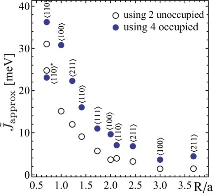
Figure 16: The effective exchange constant as estimated by the FM/AFM difference of the 4 occupied and the 2 unoccupied acceptor levels.

In Fig. 16 we plot the spherical averages of the effective $J$ as estimated by the FM/AFM difference of the sums of the 4 occupied impurity levels and the 2 unoccupied levels. Comparing with the “exact” $\tilde{J}$ calculated by total energy difference of the full system of electrons (Fig. 14), we see that both approximations underestimate the value of $\tilde{J}$ for the most closely spaced $\langle 110\rangle$ Mn pair. For the rest of the points, using the four highest occupied levels overestimates the value of $\tilde{J}$ approximately by a factor of two. Surprisingly, taking the difference of the sums of the two acceptors in the FM and the AFM configurations, gives a very good estimate of the “exact” $\tilde{J}$ for the rest of the points in the plot of Fig, 14 (a). In order to compute the effective $\tilde{J}$ for the two acceptors, one must invert the sign, because 2 unoccupied levels are used.

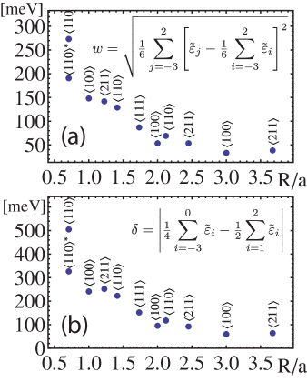
Figure 17: Six impurity level bandwidth (a), and splitting between the mean of the four occupied and the mean of the two unoccupied impurity levels (b).

In our discussion of the toy model, we have seen that the emergence of a stable FM configuration for the Mn pair is brought about by the “widening” of a partially occupied cluster of impurity levels caused by hopping. It is therefore instructive to compare some measures of the “bandwidth” of the six impurity levels with $J$. Fig. 17 (a) shows the FM effective bandwidth of the six impurity levels,

$$w=\sqrt{\tfrac{1}{6}\sum_{j=-3}^{2}\left[\tilde{\varepsilon}_{j}-\tfrac{1}{6}\sum_{i=-3}^{2}\tilde{\varepsilon}_{i}\right]^{2}},$$ (9)

and Fig. 17 (b) shows the splitting between the mean of the four occupied impurity levels and the mean of the two unoccupied levels,

$$\delta=\left|\tfrac{1}{4}\sum_{i=-3}^{0}\tilde{\varepsilon}_{i}-\tfrac{1}{2}\sum_{i=1}^{2}\tilde{\varepsilon}_{i}\right|.$$ (10)

In the FM configuration these can both be seen as a measure of the effective exchange interaction strength. A comparison of Figs. 17 and 14 reveals that they both do quite well in reproducing the correct trend in $J$, with the exception of  the most closely spaced $\langle 110\rangle$ pair. These observations support the validity of the simplified arguments used in the toy model.

In conclusion, our analysis of the acceptor splitting versus effective exchange constant shows that these two quantities are certainly related but not in a direct quantitative way. In particular, the acceptor splitting is much more anisotropic than $J$ as a function of the Mn pair orientation. Other quantities such as $w$ and $\delta$ [see Eqs. (9) and (10)] involving all six impurity levels seems have a much better correspondence with $J$. It is interesting to ask whether or not the four occupied impurity levels are also accessible by STM. One might naively expect that when the applied bias is reversed, electrons tunneling out of the occupied impurity levels should appear as sharp features in the differential conductance spectrum. The experiments of Ref. [Kitchen et al., 2006] do not show any clear sign of these levels. However, a more recent studyGupta (2009) on individual Mn impurities in GaAs indicates that a weak feature due to tunneling out of one the three $t_{2g}$ levels can indeed be seen below the top of the valence band. Presumably this is due to a hole-hole interaction effect: the final state has two electrons missing near the Mn impurity. This feature is very hard to see, as it is masked by electrons tunneling out of the valence band continuum.

III.1.4 Comparison with ab initio estimates of the exchange coupling $J$

In this section we compare our results for the effective exchange $J$ with those of previous studies. Since the pair exchange interaction between impurities is a crucial quantity in the field of DMS, there have been many theoretical studies of this quantity, mainly based on first-principles calculations. Here we concentrate our attention on a few issues that have emerged from our theoretical approach: (i) the relatively large value for the $\langle 110\rangle$ pair with shortest Mn spacing; (ii) the non-monotonic decay of $J$ with Mn separation and its strongly anisotropic character with respect to pair orientation; (iii) the comparison with acceptor splitting, with particular reference to the discrepancies between $J$ and $\Delta_{\mathrm{acc}}$ found in our model, e.g., for the $\langle 100\rangle$ pairs. A few caveats are necessary before comparing our results with other estimates of $J$ that have appeared in the literature. Firstly, most of the published estimates are for much higher Mn concentrations, which strongly affects the value of $J$ and its anisotropic properties. Secondly, all first-principle calculations suffer from the well-known limitations of DFT when applied to semiconductors. In particular, the estimates of $J$ depend on the version of DFT used, e.g. LSDA vs. GGA. When the GGA+U approach is used to account for electronic correlation effects, the value of the parameter $U$, which has as strong influence on the results, can only be determined indirectly by comparing with experiment.

In Ref. [Kudrnovsky et al., 2004] the electronic structure of (Ga,Mn)As was calculated from first principles including disorder via the coherent-potential approximation. The magnetic force theorem and one-electron Greens functions then allow mapping onto an effective Heisenberg Hamiltonian. Their results for the exchange interaction strength reveal a strong dependence on the doping concentration $x$. In particular, the effective $J$ of the nearest $\langle 110\rangle$ pair is highly sensitive to doping and increases dramatically with decreasing Mn concentration, ranging from $J=19$ meV for $x=0.08$ to $J=55$ meV for $x=0.001$. The lowest concentration of 0.1% Mn, agrees very well with our estimate. Note that our calculations correspond to a slightly smaller effective Mn concentration $x=0.0006$. In Ref. [Schilfgaarde and Mryasov, 2001] the authors employed a self-consistent LSDA atomic-spheres approximationAndersen (1975) and their result of the effective $J=55$ meV for the $\langle 110\rangle_{d=0.71a}$ pair agrees remarkably well with our values, despite the small supercell corresponding to $x=0.009$. With spin-orbit interaction this value drops to 48 meV. In Ref. [Mahadevan et al., 2004] the authors employ the GGA+U method within the Projector Augmented Wave (PAW) ab initio approach, treating $U$ as a parameter. For $\langle 110\rangle_{d=0.71}$ and $x=0.03$ they observe a decreasing $J$ as a function of $U$, with $J=34$ meV for $U=0$ and $J=22$ meV for $U=6$ eV. As the Mn concentration is reduced from $x=0.03$ to $x=0.008$ at $U=0$, an increase in $J$ of approximately 10 meV is observed. A larger $U$ parameter causes the $d$ levels to emerge deeper in the valence band, the acceptor wave function becomes more delocalized and $p$-$d$ exchange decreasesSandratskii et al. (2004). Photoemission experimentsOkabayashi et al. (1999) indicate that the $t_{2g}$-states should be approximately 4 eV below the valence band maximum, which corresponds to $U=3-4$ eV. Ref. [Mahadevan et al., 2004] shows that the calculated $J$ depends on the extension of the hole wave function as per chosen $U$.

We now turn to the $\langle 100\rangle_{d=a}$ pair, which has a very low experimental acceptor splitting (see Fig. 13). In contrast to our results (see Fig. 14), ab initio calculations generally predictKudrnovsky et al. (2004); Bergqvist et al. (2005); Hilbert and Nolting (2005); Mahadevan et al. (2004) a dip in the curve of $J$ vs Mn separation occurring for this pair, with a lower value than the two following points, $\langle 211\rangle_{d=1.21a}$ and $\langle 110\rangle_{d=1.41a}$. Similar but smaller dips are also found for the other $\langle 100\rangle$ pairs. However, as mentioned above, all these calculations show a significant dependence on impurity concentration. For example, Ref. [Kudrnovsky et al., 2004] finds that the value of $J$ for the $\langle 100\rangle_{d=a}$ pair steadily increases from approximately $J=1$ meV for $x=0.1$, to $J=7$ meV for $x=0.02$. So do the next two points for $\langle 211\rangle$ and $\langle 110\rangle$ which end up at approximately 10 meV and 11 meV for $x=0.02$. When $U=0$ and $x=0.008$, the GGA + U approach finds $J=6$ meV, well below the values for the next two pairs $\langle 211\rangle_{d=1.21a}$ and $\langle 110\rangle_{d=1.41a}$, $J=14$ meV and $J=9$ meV respectively, which are also comparable to our results. Upon increasing $U$ to the physically reasonable value of 6 eV, for both $\langle 211\rangle_{d=1.21a}$ and $\langle 110\rangle_{d=1.41a}$ $J=7$ meV, while $J=3.5$ meV for the $\langle 100\rangle_{d=a}$ pair.

For even larger values of $U$ the difference in $J$ between the $\langle 100\rangle_{d=a}$ and $\langle 211\rangle_{d=1.21a}$ pairs decreases further; however, the $\langle 100\rangle_{d=a}$ is still consistently lower. The GGA+U values of $J$ for $\langle 110\rangle_{d=1.41a}$ and $\langle 211\rangle_{d=1.21a}$, do not agree with the experimental acceptor splitting trend for sound values of $U$. A similar trend for GGA calculations is reported in Refs. [Mahadevan and Zunger, 2004; da Silva et al., 2005]. The LDA resultsSato et al. (2004) for 1% Mn including disorder in the coherent-potential approximation agree reasonably well with our results for $\langle 100\rangle_{d=a}$, $\langle 211\rangle_{d=1.21a}$ and $\langle 110\rangle_{d=1.41a}$ with $J=8.2$, 9.1 and 7.9 meV. The $\langle 100\rangle_{d=a}$ is still consistently lower for larger distances and the $\langle 110\rangle_{d=0.71a}$ is relatively low at $J=18$ meV, indicating a sensitivity of $J$ on the chosen ab initio method.

In summary, with the caveats mentioned above, the general trend of the ab initio $J$ at reduced concentrations shows some qualitative agreement with STM experimental acceptor splittings at shortest distances $d=0.71a$, $d=a$. For larger Mn separations the agreement is not so good. As corresponding theoretical estimates of the splittings are not reported in the literature, it is hard to conclude whether or not a relationship between the acceptor splittings and $J$ is present in the ab initio calculations. Concerning the comparison between the ab initio values of $J$ and our results, we can see that although the overall magnitudes agree reasonably well, the qualitative trend differs since at short Mn separations we find a monotonic decrease of $J$ with distance.

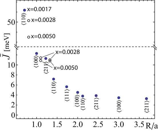
Figure 18: The effect on $\tilde{J}$ when increasing the Mn concentration from $x=0.0006$ (shown in Fig. 14) to $x=0.0017$ (filled circles). The empty circles show how $\tilde{J}$ changes when increases $x$ further for selected points.

Given the strong dependence of $J$ on Mn concentration and the fact that the reported ab initio results are obtained for larger concentrations, it is interesting to investigate how our value of $J$ changes when we increase the Mn concentration. In Fig. 18 the effect of decreasing the supercell size such that the Mn concentration changes from $x=0.0006$ to $x=0.0017$ is shown. The $\langle 100\rangle_{d=a}$ $J$ is now closer to the $\langle 211\rangle_{d=1.21a}$ value. Increasing the concentration further causes the two pairs to obtain equal $J$, but the $\langle 100\rangle_{d=a}$ value never drops below the $\langle 211\rangle_{d=1.21a}$ value, indicating that there is a fundamental difference with respect to ab initio.

Generally, ab initio predicts a qualitative trend that agrees better with our effective $J$ obtained by occupying the lower acceptor (see Fig. 15). The $\langle 100\rangle_{d=a}$ highest occupied level and lower acceptor are quasi-degenerate, with a gap that varies between 14-46 meV. In ab initio methods, a common technique used to speed up evaluation of k-point sums, is to introduce a fractional occupation of the unoccupied levels controlled by an occupation smearing parameter. At the end of the calculation, the limit of zero smearing is taken to calculate the total ground state energy. It is still possible that the end result depends on the choice of smearing parameter. If this is the case, the effect can cause the $J$ for the quasi-degenerate $\langle 100\rangle_{d=a}$ to decrease.

III.2 Mn-Mn interactions in the (110) GaAs surface

So far we have studied Mn pairs embedded in bulk GaAs. In this last Section we consider the experimentally more relevant situation where the two Mn atom substitute two Ga atoms on the $(110)$ surface. We consider again a 3200-atom supercell, but this time we apply periodic only in the two directions in the plane of the $(110)$ surface. This corresponds to a $38\times 38$ A² surface and a supercell cluster that has 20 atomic layers along the surface normal separating the two (110) surfaces, such that surface-surface interactions are negligible. The loss of coordination and hybridization with the surface states will cause the impurity levels to appear very deep in the gap. The depth is subject to experimental uncertainty due to a band-bendingWijnheijmer et al. (2009) effect when imaging a semi-conductor surface with a metal tip. In our model, the depth is very sensitive to the off-site Coulomb correction, $V_{\mathrm{off}}$, and we use this parameter to reproduce the acceptor level of a single Mn on the (110) surface at the experimentally observed positionKitchen et al. (2006) at 850 meV. The parameter $V_{\mathrm{off}}$ has therefore been reduced from 2.4 eV to 1.57 eV.

We proceed again to study the magnetic anisotropy energy of the systems, the properties of the mid-gap acceptor states, the effective exchange interaction and its connection with the acceptor splitting.

III.2.1 Magnetic anisotropy energy

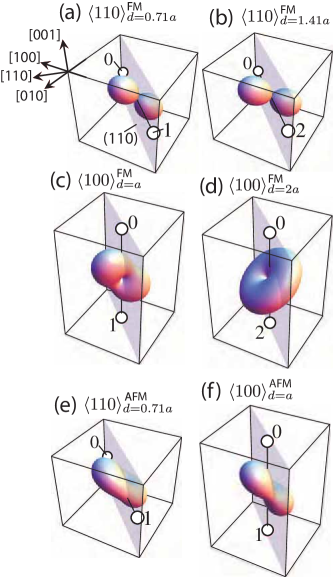
Figure 19: (Color online) The magnetic anisotropy landscapes for Mn pairs in the (110) surface. The transparent plane indicates the (110) surface. (a)-(d) show the distinct types of landscapes in the FM configurations. Only along the $\langle 110\rangle_{d=0.71a,1.41a}$ in (a) and (b), and $\langle 100\rangle_{d=a}$ in (c), do the landscapes differ from the result of weakly interacting pairs in (d), which is just the sum of two isolated Mn anisotropies. Similarly, in the AFM configurations, only $\langle 110\rangle_{d=0.71a}$ (e) and $\langle 100\rangle_{d=a}$ (f) deviate qualitatively from the landscape (d).

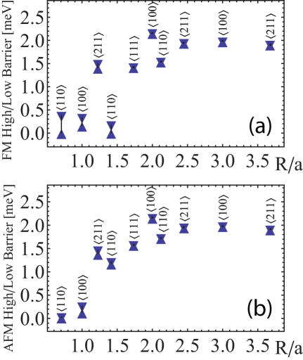
Figure 20: The high and low barriers for the FM (a) and the AFM (b) configurations for pairs at the (110) surface. The anisotropy for the closest pairs exhibit a reduced anisotropy energy for separations greater than two lattice constants, all pairs have a characteristic barrier of around 2 meV, indicative of very weakly interacting Mn.

Fig. 19 shows the qualitatively distinct anisotropy landscapes for Mn pairs on the surface and Fig. 20 the magnitude of the barriers. The surface geometry completely dominates the anisotropy and for most separations the anisotropy landscape is qualitatively the same as for a single Mn in the surfaceStrandberg et al. (2009) [exemplified in Fig. 19 (d)]. This type of anisotropy landscape occurring for separations larger than $\approx 1.5$ lattice constants is an indication that the acceptor state hybridization is so weak that the resulting anisotropies are essentially the sum of two independent Mn atom anisotropies. Only for the closest pairs do different anisotropies appear. In the FM configurations only $\langle 110\rangle_{d=0.71a}$, $\langle 110\rangle_{d=1.41a}$ and $\langle 100\rangle_{d=a}$ [Fig. 19 (a)-(c)] show qualitatively different landscapes - tilted quasi-easy planes with the hard direction approximately along [111]. Similarly for the AFM configurations, only $\langle 110\rangle_{d=0.71a}$ and $\langle 100\rangle_{d=a}$ [Fig. 19 (e)-(f)] differ from the single Mn type landscape in Fig. 19 (d). In $\langle 100\rangle_{d=a}$ the easy axis and the low barrier are interchanged between the AFM and FM, but the hard direction remains along the [111].

Fig. 20 shows that anisotropy energies are very small, typically one order of magnitude smaller than for the fully periodic systems. In both FM and AFM configurations the interactions between Mn for distances below two lattice constants, tend to reduce the anisotropy heavily. At larger distances, where all Mn pairs produce the [111] easy axis type landscape in Fig. 19 (d), the single barriers are around 2 meV. This limit of weakly interacting Mn is also reflected in the difference in barriers (see 20) between the FM and AFM, which becomes negligible for weakly hybridized pairs above $1.5a$. As we will show, total energy differences are also small, causing a very small effective exchange.

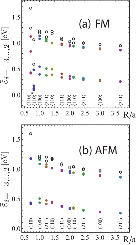
Figure 21: The four highest occupied (filled circles) and the two acceptor levels (empty circles) in the FM (a) and AFM (b) configuration for Mn pairs in the (110) surface. Loss of coordination and hybridization with surface states cause impurity levels deep in the gap.

III.2.2 Character of acceptor levels for Mn pairs in a (110) surface

Fig. 21 shows the group of six impurity levels for the Mn pairs in the surface. We see that for both FM and AFM configurations, two of the occupied levels are split around 0.5 eV below the others. For the closest $\langle 110\rangle$ pair the acceptors are so high in energy that the upper acceptor has in fact crossed the first conduction band state. This is associated with a very large splitting of the acceptors. In $\langle 110\rangle^{R}$ the off-site Coulomb has been reduced even further (to 0.5 eV) in order to also make the upper acceptor appear in the gap. The overall spectrum for the AFM and FM configuration looks similar, indicating that interactions are very weak and the itinerant spin wave functions are very localized at the surface. In the STM experimentKitchen et al. (2006) Zn dopants can give rise to resonant tunneling between conduction states and the acceptor level, thought to be responsible for the negative dip seen in the curve of the tunneling conductance vs. bias voltage.Loth et al. (2006) The coupling to conduction-like states can lead to a more extended, bulk-like acceptor wave function seen at the (110) surface. As a first approximation our treatment of the surface should reveal some of the relevant properties. Our results indicate that the interactions in the surface are much weaker than in bulk, and magnetic anisotropies are one order of magnitude smaller. This is related to acceptor wave functions that are much more localized at the surface.

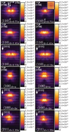
Figure 22: (Color online) LDOS for FM aligned Mn pairs on the (110) surface. The inset in $\langle 110\rangle^{R}$ shows the level above the low acceptor when the upper acceptor has crossed into the conduction band. The images are for the Mn spin in the easy direction, indicated in the top left corner of each panel (note that [111] is coming out of the (110) surface).

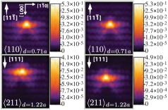
Figure 23: (Color online) Examples of LDOS for AFM aligned pairs Mn in the (110) surface.

So far there are relatively few papers that attempt to simulate STM images of Mn in the (110) surface.Mikkelsen et al. (2004); Stroppa et al. (2007) The acceptor LDOS resulting from our tight-binding model for a few representative pairs are shown in Fig. 22 for the FM and Fig. 23 for the AFM configurations. The spectral weight in the core regions of the Mn are much higher than in bulk. As an example, the upper acceptor for the $\langle 110\rangle_{0.71a}^{R}$ has around 50% spectral weight on the As in-between the Mn, to be compared with 17% in bulk, which is still high relative other bulk configurations. Wave functions for other surface pairs have a much higher maximum spectral weight than in bulk, with values in the typical range 20%-30%. Overall, the spectral weight maximum for a given pair in bulk is approximately an order of magnitude smaller than the corresponding pair at the surface, with bulk wave functions that are much more spread out in the lattice.

As shown in the first two rows of Fig. 22, some bonding/antibonding characteristics in the acceptor wave functions can be seen for the closest pairs $\langle 110\rangle_{d=0.71a,1.41a}$ in the FM configuration, which exhibit magnetic quasi-easy planes. Both acceptor wave functions for the $\langle 110\rangle_{d=2.12a}$ Mn pair exhibit a hint of antibonding character. Note that this pair is characterized by the magnetic anisotropy landscape of a single Mn impurity.

For $\langle 100\rangle_{d=a}$ each acceptor level is occupying both Mn sites, but a separation occurs for $\langle 100\rangle_{d=2a,d=3a}$ such that each acceptor has more pronounced LDOS on one of the sites. The same association of acceptors spatially bound to one site, appears for the other directions - a pattern indicative of weak hybridization. Finally the $\langle 211\rangle_{d=1.22a}$ has some hint of bonding/antibonding pattern, but not as pronounced as for bulk.

In the LDOS for the AFM configurations (see Fig. 23), the $\langle 110\rangle$ pairs show no spatial separation between the acceptors and no bonding/antibonding behavior. The $\langle 211\rangle_{d=1.22a}$ has upper and lower acceptor wave functions that are localized to the separate Mn sites, whereas the rest of the pairs are similar to the bulk counterparts (see Fig. 12), but with a more localized LDOS signature.

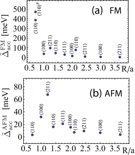
Figure 24: The splittings of the acceptor levels for Mn pairs in the (110) surface.

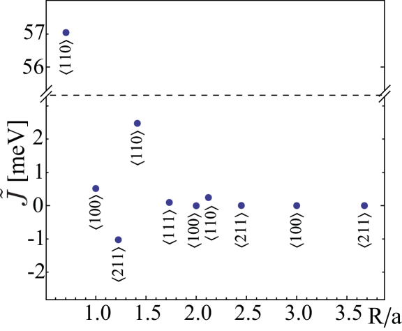
Figure 25: The effective exchange constant for Mn pairs in the (110) surface. The effective $\tilde{J}$ falls off much faster at the surface, due to the highly localized acceptor wave functions. The $\langle 211\rangle_{d=1.22a}$ is showing antiferromagnetic behavior.

III.2.3 Acceptor splitting vs. effective exchange constant $J$

Finally, we have calculated the effective exchange constant for the Mn pairs in the surface, which we compare with the calculated acceptor splittings. The FM splittings of the acceptor levels is shown in Fig. 24 (a). The very large splitting of 600 meV for the closest Mn pair seen in experiment (see Fig. 13) is now comparable to the calculated one of around 500 meV, when both acceptors are in the gap. The calculated splitting is small for the nearest $\langle 100\rangle$. It then increases to around 100 meV for the $\langle 211\rangle$, but after that splittings are very small and less than 50 meV, with the exception of the farthest $\langle 110\rangle$. In the AFM configurations, splittings are much larger at the surface compared to bulk. In particular, the closest $\langle 211\rangle$ has a large splitting of around 70 meV. This is expected, since a finite splitting in the AFM configuration is possible when inversion symmetry is broken, an effect that is clearly enhanced by the presence of the surface.

The FM surface splittings do not match the long range experimental trend as well as the bulk calculations. In our calculations, we have accounted for the buckling of the GaAs (110) surface, but not the detailed relaxation of Mn environment. It is also not certain that the effective $p$-$d$ exchange model holds so well for the surface. Not only the long range and short range Coulomb may differ at the surface, but the exchange splitting is also subject to change. This is because the $p$-$d$ hybridization scheme in Fig. 1 will be altered by the surface states.

The surface $\tilde{J}$ are shown in Fig. 25. For the nearest $\langle 110\rangle$ pair, $\tilde{J}$ is strongly ferromagnetic and has a value similar to the corresponding pair in bulk. The $\langle 100\rangle$ pair has a very low $\tilde{J}$ of around half an meV and could easily become antiferromagnetic by a change in Coulomb parameters. The SO-induced anisotropy of $J$ on the unit sphere of magnetic moment directions is very weak, just fractions of an meV, due to the low anisotropy energies at the surface. Interestingly the $\langle 211\rangle$ pair, which has a relatively large acceptor splitting of several tens meV in the AFM configuration (see Fig. 24), is antiferromagnetic. As mentioned above, this is an effect entirely due to the surface, where a significant acceptor splitting can exist even for antiferromagnetically aligned Mn spins and generate an energy gain that can compete with the FM configuration. The rest of the Mn pairs shown in Fig. 25 have a very small $\tilde{J}$, indicating that the Mn local moments interact very weakly due to the high degree of localization of the acceptor wave functions at the surface. The oscillatory behavior is indicative of Friedel oscillations with a much shorter period than in bulk, which is connected to the strong localization of the acceptor wave functions at the surface. Finally, it is interesting to note that the magnitude of $\tilde{J}$ (disregarding the sign), follows the trend of the experimentally observed splittings, despite the fact that the calculated ones do not clearly do so. Disregarding the single point $\langle 110\rangle_{d=1.41a}$ in Fig. 24 (a), the experimental trend but with smaller magnitudes is reproduced. It is also interesting to note the large AFM splitting for $\langle 211\rangle_{d=1.22a}$ in Fig. 24 (a), which makes it difficult to distinguish from the FM configuration. There are however noticeable differences between the $\langle 211\rangle_{d=1.22a}$ FM and AFM LDOS (see Figs. 22 and 23). The FM acceptors each have spectral weight on both Mn sites, but the AFM acceptors are each associated with one site. Given the large splitting between the AFM acceptors, this observation could perhaps be tested experimentally. Overall, it would appear that the experimental results for the (110) surface are intermediary to our surface and bulk calculations.

IV Conclusions and Outlook

In this paper we have investigated substitutional Mn pairs in GaAs, using a microscopic tight-binding model solved for large GaAs clusters. The model accounts realistically for spin-orbit interactions and includes the kinetic-exchange $p$-$d$ coupling between the Mn local magnetic moment and the spin of valence band electrons. One goal of this work was to assess whether or not this model can reproduce the main features of coupled acceptor states observed in recent STM experiments,Kitchen et al. (2006, 2007) and in this way further elucidate the nature of the effective exchange interaction between the two Mn magnetic moments. When the two Mn atoms are located in the bulk, we find that the ground state of the system is generally one in which the two Mn magnetic moments are coupled ferromagnetically and aligned along the direction connecting the Mn atoms. In the ferromagnetic configuration, the two topmost acceptor states are split, and their energy separation depends strongly on the Mn pair orientation with respect to the GaAs crystal structure and decreases with Mn separation. In particular, the largest splitting ($\sim 300$ meV) is found for the Mn pair oriented along the $\langle 110\rangle$ direction. For separations larger than three lattice constants, the splitting is below 20 meV. The splitting is the result of hybridization of degenerate acceptor states with identical spin character, giving rise to bonding and antibonding states. Our calculated acceptor splittings are typically a factor of two smaller than the experimental values. Coulomb correlation effects not included in our tight-binding approach could partly be responsible for the larger splittings. Analysis of the LDOS for the two acceptor states shows that these are mainly concentrated in the surroundings of the Mn atoms; for intermediate separations, when the splitting is sizable, the higher state and lower state are of the bonding and anti-bonding type respectively. These results are all consistent with experiment,Kitchen et al. (2006, 2007) indicating that the TB model correctly describes the electronic properties of the coupled acceptor states in GaAs associated with the magnetic impurities.

An important question that we have addressed here is whether or not the acceptor splitting, which is accessible by STM measurements, is directly related to the effective exchange coupling between the Mn local moments. The present work demonstrates that, at least within the model considered here, this relationship is not very sharp: although both quantities decrease with separation and are typically anisotropic, the acceptor splitting displays a non-monotonic behavior for a few pair orientations which is not found in the exchange coupling. In our model, the dependence of the latter on Mn separation and pair orientation is better represented by the overall bandwidthendnote50 of the six impurity levels present in the gap (see Fig. 17). In particular, Our calculations demonstrate that exchange interactions between two Mn ions in (Ga,Mn)As are closely related to the splitting between the two acceptor levels that are occupied by holes and the four lower energy acceptor levels that are occupied by electrons. This splitting is not readily measured by STM experiments which are strongly influenced by Coulomb interaction energies when the number of holes bound to the acceptor complex is increased above two by removing electrons from the system. It is possible that infrared spectroscopy of transitions between iso-charge levels of the acceptor complex could be more effective.

These results support the idea that the stability and strength of the ferromagnetic coupling involves the hybridization of all impurity levels and not only the two topmost ones occupied by holes. Our estimate of the exchange coupling is in qualitative agreement with results obtained from ab initio calculations, with a few noticeable discrepancies analyzed in detailed in Sec. III.1.4, which are most likely due to the limitations of both methods and deserve further investigation.

When the two Mn atoms are inserted in the $(110)$ surface as in experiment, we typically find much deeper acceptor states with strongly localized wave functions around the impurities. Weaker hybridization causes the acceptor splitting to decay more rapidly with separation, although in a manner qualitatively similar to bulk. With the exception of the most closely spaced Mn pair, the surface acceptor splittings seem to agree less well with experiment than our bulk results. The exchange constant is likewise very small except at the shortest separations and can even change sign, favoring an antiferromagnetic coupling. These results are a clear indication that our semiphenomenological microscopic model, derived mainly from bulk (Mn,Ga)As properties, is not able to quantitatively capture the complexity of the surface states. This is an area that could benefit from additional work.

The model investigated here makes predictions for the spin-orbit induced magnetic anisotropy for pairs of Mn atoms in GaAs. Some of these predictions could be tested in STM experiments by applying an external field. When the Mn pair is in a bulk environment, there is a uniaxial magnetic anisotropy along the axis of the pair with anisotropy barriers of 10-20 meV. When the pair is in a (110) surface, the behavior of the anisotropy energy landscape is for most pairs similar in character and magnitude to that of a single Mn atom in the (110) surface.Strandberg et al. (2009).

In the present approach the local moment degrees of freedom have been treated as classical variables. The study of the quantum spin dynamics of two interacting Mn in GaAs is an important and interesting subject both theoretically and in view of future experiments. Work in this direction, based on Berry-phase quantization of the semi-classical local moments considered here, is underway.

V Acknowledgments

This work was supported by the Welch Foundation and the National Science Foundation under grant DMR-0606489, the Faculty of Natural Sciences at Kalmar University, the Swedish Research Council under Grant No: 621-2004-4439, and by the Office of Naval Research under grant N00014-02-1-0813. We would like to thank J. Gupta, A. Yazdani, P. M. Koenraad, J. K. Garleff, A. P. Wijnheijmer and C. F. Hirjibehedin for useful discussions.

References

- (1)
- (2)
- (3)
- (4)
- Yakunin et al. (2004) A. M. Yakunin, A. Y. Silov, P. M. Koenraad, W. V. Roy, J. D. Boeck, J.-M. Tang, and M. E. Flatté, Phys. Rev. Lett 92, 216806 (2004).
- Yakunin et al. (2005) A. M. Yakunin, A. Y. Silov, P. M. Koenraad, J.-M. Tang, M. E. Flatté, W. V. Roy, J. D. Boeck, and J. H. Wolter, Phys. Rev. Lett 95, 256402 (2005).
- Kitchen et al. (2005) D. Kitchen, A. Richardella, and A. Yazdani, J. Supercond. 18, 23 (2005).
- Kitchen et al. (2006) D. Kitchen, A. Richardella, J.-M. Tang, M. E. Flatté, and A. Yazdani, Nature 442, 436 (2006).
- Kitchen et al. (2007) D. Kitchen, A. Richardella, P. Roushan, J.-M. Tang, M. E. Flatté, and A. Yazdani, Jour. App. Phys. 101, 515 (2007).
- Garleff et al. (2008) J. K. Garleff, C. Celebi, W. van Roy, J.-M. Tang, M. E. Flatté, and P. M. Koenraad, Phys. Rev. B 78, 075313 (2008).
- Richardella et al. (2009) A. Richardella, D. Kitchen, and A. Yazdani, Phys. Rev. B 80, 045318 (2009).
- Dietl (2008) T. Dietl, Spintronics (Elsevier Science, 2008), vol. 82 of Semiconductor and Semimetals, chap. 9.
- Schilfgaarde and Mryasov (2001) M. Schilfgaarde and O. N. Mryasov, Phys. Rev. B 63, 233205 (2001).
- Strandberg et al. (2009) T. O. Strandberg, C. M. Canali, and A. H. MacDonald, Phys. Rev. B 80, 024425 (2009).
- Zhao et al. (2004) Y. Zhao, P. Mahadevan, and A. Zunger, Apl. Phys. Lett. 84, 3753 (2004).
- Jungwirth et al. (2006) T. Jungwirth, J. Sinova, J. Masek, J. Kucera, and A. H. MacDonald, Rev. Mod. Phys. 78, 809 (2006).
- Vogl and Baranowski (1985) P. Vogl and J. M. Baranowski, Acta Phys. Pol. A 67, 133 (1985).
- Zener (1951) C. Zener, Phys. Rev. 81, 440 (1951).
- Dietl et al. (2000) T. Dietl, H. Ohno, F. Matsukura, J. Cibert, and D. Ferrand, Science 287, 1019 (2000).
- Bhattacharjee et al. (1983) A. Bhattacharjee, G. Fishman, and B. Coqblin, Physica B & C 117-118, 449 (1983).
- Okabayashi et al. (1998) J. Okabayashi, A. Kimura, O. Rader, T. Mizokawa, A. Fujimoro, T. Hayashi, and M. Tanaka, Phys. Rev. B 58, R4211 (1998).
- Chadi (1977) D. J. Chadi, Phys. Rev. B 16, 790 (1977).
- Slater and Koster (1954) J. C. Slater and G. F. Koster, Phys. Rev. 94, 1498 (1954).
- Papaconstantopoulos and Mehl (2003) D. A. Papaconstantopoulos and M. J. Mehl, J. Phys.: Cond. Mat. 15, R413 (2003).
- Chadi (1978) D. J. Chadi, Phys. Rev. Lett. 41, 1062 (1978).
- Chadi (1979) D. J. Chadi, Phys. Rev. B 19, 2074 (1979).
- Timm and MacDonald (2005) C. Timm and A. H. MacDonald, Phys. Rev. B 71, 155206 (2005).
- Ohno (1998) H. Ohno, Science 281, 951 (1998).
- Schairer and Schmidt (1974) W. Schairer and M. Schmidt, Phys. Rev. B 10, 2501 (1974).
- Lee and Anderson (1964) T. Lee and W. W. Anderson, Solid State Commun. 2, 265 (1964).
- Chapman and Hutchinson (1967) R. A. Chapman and W. G. Hutchinson, Phys. Rev. Lett. 18, 443 (1967).
- Linnarsson et al. (1997) M. Linnarsson, E. Janzen, B. Monemar, M. Kleverman, and A. Thilderkvist, Phys. Rev. B 55, 6938 (1997).
- Anderson and Hasegawa (1955) P. W. Anderson and H. Hasegawa, Phys. Rev. 100, 675 (1955).
- Chiba et al. (2009) D. Chiba, M. Sawicki, Y. Nishitani, Y. Nakatani, F. Matsukura, and H. Ohno, Nature 455, 515 (2008).
- Zemen et al. (2009) J. Zemen, J. Kucera, K. Olejnik, and T. Jungwirth, Phys. Rev. B 80, 155203 (2009).
- (36) R. Wiesendanger, Rev. Mod. Phys. 81, 1495 (2009).
- Tang and Flatté (2004) J.-M. Tang and M. E. Flatté, Phys. Rev. Lett. 92, 047201 (2004).
- Gupta (2009) J. Gupta, private communication, (2009).
- Kudrnovsky et al. (2004) J. Kudrnovsky, I. Turek, V. Drchal, F. Maca, P. Weinberger, and P. Bruno, Phys. Rev. B 69, 115208 (2004).
- Andersen (1975) O. K. Andersen, Phys. Rev. B 12, 3060 (1975).
- Mahadevan et al. (2004) P. Mahadevan, A. Zunger, and D. D. Sarma, Phys. Rev. Lett. 93, 177201 (2004).
- Sandratskii et al. (2004) L. M. Sandratskii, P. Bruno, and J. Kudrnovsky, Phys. Rev. B 69, 195203 (2004).
- Okabayashi et al. (1999) J. Okabayashi, A. Kimura, O. Rader, T. Mizokawa, A. Fujimoro, T. Hayashi, and M. Tanaka, Phys. Rev. B 59, 2486 (1999).
- Bergqvist et al. (2005) L. Bergqvist, O. Eriksson, J. Kudrnovsky, V. Drchal, A. Bergman, L. Nordstrom, and I. Turek, Phys. Rev. B 72, 195210 (2005).
- Hilbert and Nolting (2005) S. Hilbert and W. Nolting, Phys. Rev. B 71, 113204 (2005).
- Mahadevan and Zunger (2004) P. Mahadevan and A. Zunger, Appl. Phys. Lett. 85, 2860 (2004).
- da Silva et al. (2005) A. da Silva, A. Fazzio, R. Santos, and L. E. Oliveira, Phys. Rev. B 72, 125208 (2005).
- Sato et al. (2004) K. Sato, W. Schweika, P. H. Dederichs, and H. Katayama-Yoshida, Phys. Rev. B 70, 201202 (2004).
- Wijnheijmer et al. (2009) A. P. Wijnheijmer, J. K. Garleff, K. Teichmann, M. Wenderoth, S. Loth, R. G. Ulbrich, P. Maksym, M. Roy, and P. M. Koenraad, Phys. Rev. Lett. 102, 166101 (2009).
- Loth et al. (2006) S. Loth, M. Wenderoth, L. Winking, R. Ulbrich, S. Malzer, and G. Dohler, Phys. Rev. Lett. 96, 066403 (2006).
- Mikkelsen et al. (2004) A. Mikkelsen, B. Sanyal, J. Sadowski, L. Ouattara, J. Kanski, S. Mirbt, O. Eriksson, and E. Lundgren, Phys. Rev. B 70, 085411 (2004).
- Stroppa et al. (2007) A. Stroppa, X. Duan, M. Peressi, D. Furlanetto, and S. Modesti, Phys. Rev. B 75, 195335 (2007).