On the $p,q$-binomial distribution
and the Ising model

Abstract

A completely new approach to the Ising model in 1 to 5 dimensions is developed. We employ $p,q$-binomial coefficients, a generalisation of the binomial coefficients, to describe the magnetisation distributions of the Ising model. For the complete graph this distribution corresponds exactly to the limit case $p=q$. We take our investigation to the simple $d$-dimensional lattices for $d=1,2,3,4,5$ and fit $p,q$-binomial distributions to our data, some of which are exact but most are sampled. For $d=1$ and $d=5$ the magnetisation distributions are remarkably well-fitted by $p,q$-binomial distributions. For $d=4$ we are only slightly less successful, while for $d=2,3$ we see some deviations (with exceptions!) between the $p,q$-binomial and the Ising distribution. We begin the paper by giving results on the behaviour of the $p,q$-distribution and its moment growth exponents given a certain parameterization of $p,q$. Since the moment exponents are known for the Ising model (or at least approximately for $d=3$) we can predict how $p,q$ should behave and compare this to our measured $p,q$. The results speak in favour of the $p,q$-binomial distribution’s correctness regarding their general behaviour in comparison to the Ising model. The full extent to which they correctly model the Ising distribution is not settled though.

I Introduction

Choose a graph, e.g. a square lattice, on $n$ vertices and compute its Ising partition function $\mathcal{Z}$, keeping track of its terms according to their magnetisation, so that $\mathcal{Z}=\mathcal{Z}_{0}+\mathcal{Z}_{1}+\cdots+\mathcal{Z}_{n}$. The quotient $\mathcal{Z}_{k}/\mathcal{Z}$ is the probability of having $k$ negative spins, or magnetisation $M=n-2\,k$. The controlling parameter of the partition function is the temperature, that is, for any given temperature the partition function provides us with a distribution of magnetisations. At infinite temperature this is simply the binomial distribution. At zero temperature, on the other hand, we receive a distribution with two peaks, one at $k=0$ and one at $k=n$, both with 50% of the probability mass. The distribution is always symmetrical. What happens between these two extreme temperatures? Though there are exceptions to the rule, for most graphs the distribution begins its life at high temperatures as a unimodal distribution with the peak at the middle $k=n/2$. As we lower the temperature the distribution gets increasingly wider until we reach a temperature where the distribution changes from unimodal to bimodal. Near this temperature, slightly above and slightly below, the distribution is particularly wide. Lowering the temperature even further the distribution develops two sharp peaks, both essentially gaussian, and the peaks move outwards.

This article tries to model the distributions using $p,q$-binomial coefficients. In one case, the complete graph, they model exactly the distributions and for $d$-dimensional lattices the dimension seems to determine how well they fit to the Ising distributions. Especially in the case of $d=1$ and $d=5$ the Ising distributions are particularly well-fitted by the $p,q$-binomial coefficients.

The paper begins in section II by providing the necessary basic tools, such as the Pochhammer and $q$-Pochhammer symbol, $q$-binomial coefficients and finally the $p,q$-binomial coefficients. Some nice results on their properties are also stated, even though they are of no direct use to us in the rest of the paper. They are merely intended to give the reader a feel of how $p,q$-binomials behave. In section III we define the $p,q$-binomial distribution and give an algorithm for finding values of $p$ and $q$ when the distribution is given as input. The problem is to determine an optimal choice for $p$ and $q$. As it turns out we only have to focus on the value of the probability and the location of the distribution’s peaks, at least for a bimodal distribution. The unimodal distribution always has its peak at the middle so in this case we instead take the quotient between the two middle probabilities as controlling parameter. This quotient is unfortunately rather sensitive to noise, making it difficult to determine the parameters $p$ and $q$ for sampled data.

Section IV gives detailed results for the special case when $p=q$. This case corresponds exactly to the complete graph and is the only case where we can give asymptotically exact expressions for the sum of the coefficients. In section V we provide some useful tools for working with $p,q$-binomial coefficients in the case when $p\neq q$. After this build-up of tools we are, at long last, ready to give some general results on the distribution of $p,q$-binomial coefficients in section VI. Using the parameterization $p=1+y/n$ and $q=1+z/n$ we find the asymptotic value of $y$, given $z$, where the distribution is flat in the middle. We also allow for a small change in $y$, using a higher order parameter $a$, so that we can follow properly how the distribution changes from unimodal to bimodal. However, the computations that we rely on involve some rather complicated series expansions that were made using Mathematica. These are much too long to fit into this paper. We have prepared a simplified Mathematica notebook that performs all the necessary computations. The interested reader can obtain it by contacting the first author.

Section VII looks into the case of moving $y$ and $z$ along a line with any given slope as opposed to the previous section where $z$ stays fixed. In section VIII we give exact scaling formulae for the moments of the distributions depending on the parameters $a$ and $z$. For a given moment of these distributions we always obtain the same exponent on $n$, regardless of $a$ and $z$. In section IX we try to remedy this by letting the previously fixed parameter $z$ depend ever so slightly (at most logarithmically) on $n$. This is based on the assumption that the previous formulae in section VI still hold. However, we can now adjust the exponent of $n$ though this comes at the cost of an extremely slow convergence.

Section X defines the Ising model, laying the ground for studying distributions of magnetisations, the intended application of our endeavour. In section XI we apply our tools to the $d$-dimensional lattice graphs for $d=1,2,3,4,5$ fitting $p,q$-distributions to simulated distributions and comparing them.

A condensed reading, more suitable to the reader who is pressed for time, should include a look at (1), (14), (27), (28), (29), (49), (50), (51) for the necessary definitions and results concerning the basics. After that, the most important results are stated in equations (62), (65), (96), (109) and (112). After looking up the basic definitions regarding the Ising model the reader can skip to (121). In Section XI the reader can now pick and choose his favourite lattice and look at the pictures.

II Definitions, notations, the very basics

The $q$-binomial coefficient

$$\genfrac{[}{]}{0.0pt}{0}{n}{k}_{q}=\prod_{i=1}^{k}\frac{1-q^{n-i+1}}{1-q^{i}},\quad\textrm{$q\neq 1$, $0\leq k\leq n$}$$ (1)

is a natural extension of the standard binomial coefficient

$$\binom{n}{k}=\frac{n!}{k!\,(n-k)!},\quad 0\leq k\leq n$$ (2)

The Pochhammer symbol (or shifted factorial) is defined as

$$(a)_{n}=\prod_{i=0}^{n-1}(a+i)$$ (3)

so that $(1)_{n}=n!$. Its $q$-deformed relative, the $q$-Pochhammer symbol, is defined as

$$\left(a;\,q\right)_{n}=\prod_{i=0}^{n-1}\left(1-a\,q^{i}\right),\quad n\geq 0$$ (4)

The $q$-binomial coefficient can then be expressed as

$$\genfrac{[}{]}{0.0pt}{0}{n}{k}_{q}=\frac{\left(q;\,q\right)_{n}}{\left(q;\,q\right)_{k}\,\left(q;\,q\right)_{n-k}}=\frac{\left(q^{n-k+1};\,q\right)_{k}}{\left(q;\,q\right)_{k}}$$ (5)

The $q$-numbers are defined for any real number $a$ as

$$[a]_{q}=\frac{1-q^{a}}{1-q},\quad q\neq 1$$ (6)

and it is easy to show that

$$\lim_{q\to 1}[a]_{q}=a$$ (7)

Note that for integers $n\geq 1$ we have

$$[n]_{q}=\frac{1-q^{n}}{1-q}=1+q+\cdots+q^{n-1},\quad q\neq 1$$ (8)

so that $[n]_{q}\to n$ when $q\to 1$. To continue, the $q$-number factorials are defined as

$$[n]_{q}!=\prod_{k=1}^{n}[k]_{q}$$ (9)

and then obviously

$$\lim_{q\to 1}[n]_{q}!=n!$$ (10)

The $q$-binomial can now be defined in an alternative way as

$$\genfrac{[}{]}{0.0pt}{0}{n}{k}_{q}=\frac{[n]_{q}!}{[k]_{q}!\,[n-k]_{q}!}$$ (11)

and then it follows that

$$\lim_{q\to 1}\genfrac{[}{]}{0.0pt}{0}{n}{k}_{q}=\binom{n}{k}$$ (12)

Quite analogously it is easy to verify that

$$\lim_{q\to 1}\frac{\left(q^{a};\,q\right)_{n}}{(1-q)^{n}}=(a)_{n}$$ (13)

Finally, note also that $\genfrac{[}{]}{0.0pt}{0}{n}{k}_{q}$ can be viewed as a formal polynomial in $q$ of degree $k\,(n-k)$ where the coefficient of $q^{j}$ counts the number of $k$-subsets of $\{1,\ldots,n\}$ with element sum $j+k\,(k+1)/2$. It is thus a polynomial with positive coefficients.

We have so far only stated what belongs to the standard repertoire on the subject. The $q$-binomials and the $q$-Pochhammer function have many interesting properties and we point the interested reader to the books Gasper and Rahman (2004), Andrews (1976), Andrews et al. (1999) and especially the charming little book Andrews (1986). For more on the standard binomial coefficient and Pochhammer function we recommend Graham et al. (1994) which contains a wealth of useful information.

A natural extension of the $q$-binomial coefficient, the $p,q$-binomial coefficient, was defined in Corcino (2008) as

$$\genfrac{[}{]}{0.0pt}{0}{n}{k}_{p,q}=\prod_{i=1}^{k}\frac{p^{n-i+1}-q^{n-i+1}}{p^{i}-q^{i}},\quad\textrm{$p\neq q$,\, $0\leq k\leq n$}$$ (14)

Clearly, in the case $p=1$ this reduces to a $q$-binomial coefficient. Also, note that $p$ and $q$ are interchangable so that

$$\genfrac{[}{]}{0.0pt}{0}{n}{k}_{p,q}=\genfrac{[}{]}{0.0pt}{0}{n}{k}_{q,p}$$ (15)

Just as the standard binomial coefficients, their $p,q$-analogues are also symmetric

$$\genfrac{[}{]}{0.0pt}{0}{n}{k}_{p,q}=\genfrac{[}{]}{0.0pt}{0}{n}{n-k}_{p,q}$$ (16)

It is an easy exercise to show the following identity and we leave this to the reader.

$$\genfrac{[}{]}{0.0pt}{0}{n}{k}_{p,q}=p^{k\,(n-k)}\,\genfrac{[}{]}{0.0pt}{0}{n}{k}_{q/p}=q^{k\,(n-k)}\,\genfrac{[}{]}{0.0pt}{0}{n}{k}_{p/q}$$ (17)

As a corollary it follows that

$$\lim_{p,q\to r}\genfrac{[}{]}{0.0pt}{0}{n}{k}_{p,q}=r^{k\,(n-k)}\,\binom{n}{k}$$ (18)

Any identity involving $q$-binomial coefficients can then be extended to a $p,q$-binomial identity by first replacing $q$ with $q/p$ and then use the identity (17). For example, the binomial theorem

$$\left(1+x\right)^{n}=\sum_{k=0}^{n}\binom{n}{k}\,x^{k}$$ (19)

has the $q$-analogue

$$\prod_{\ell=0}^{n-1}\left(1+x\,q^{\ell}\right)=\sum_{k=0}^{n}\genfrac{[}{]}{0.0pt}{0}{n}{k}_{q}\,q^{\binom{k}{2}}\,x^{k}$$ (20)

Now replace $q$ with $q/p$ and then use the identity

$$\genfrac{[}{]}{0.0pt}{0}{n}{k}_{q/p}=p^{-k\,(n-k)}\,\genfrac{[}{]}{0.0pt}{0}{n}{k}_{p,q}$$ (21)

from (17) above. This gives us

$$\prod_{\ell=0}^{n-1}\left(1+x\,(q/p)^{\ell}\right)=\sum_{k=0}^{n}\genfrac{[}{]}{0.0pt}{0}{n}{k}_{p,q}\,p^{-k\,(n-k)}\,(q/p)^{\binom{k}{2}}\,x^{k}$$ (22)

After multiplying both sides with $p^{\binom{n}{2}}$ this simplifies into

$$\prod_{\ell=0}^{n-1}\left(p^{\ell}+x\,q^{\ell}\right)=\sum_{k=0}^{n}\genfrac{[}{]}{0.0pt}{0}{n}{k}_{p,q}\,p^{\binom{n-k}{2}}\,q^{\binom{k}{2}}\,x^{k}$$ (23)

which was also shown in Corcino (2008) using a recursion technique.

As another application we consider the Chu-Vandermonde identity

$$\binom{m+n}{k}=\sum_{\ell=0}^{k}\binom{m}{k-l}\,\binom{n}{\ell}$$ (24)

which is a fairly direct consequence of the binomial theorem applied to the product $(1+x)^{m}\,(1+x)^{n}$. The $q$-Vandermonde identity, see e.g. Gasper and Rahman (2004) and (though misprinted) Corcino (2008), can be stated as

$$\genfrac{[}{]}{0.0pt}{0}{m+n}{k}_{q}=\sum_{\ell=0}^{k}\genfrac{[}{]}{0.0pt}{0}{m}{k-\ell}_{q}\,\genfrac{[}{]}{0.0pt}{0}{n}{\ell}_{q}\,q^{\ell\,(m-k+\ell)}$$ (25)

Using (17) above we can now obtain a $p,q$-analog of this.

Theorem II.1.

$$\genfrac{[}{]}{0.0pt}{0}{m+n}{k}_{p,q}=\sum_{\ell=0}^{k}\genfrac{[}{]}{0.0pt}{0}{m}{k-\ell}_{p,q}\,\genfrac{[}{]}{0.0pt}{0}{n}{\ell}_{p,q}\,p^{(n-\ell)\,(k-\ell)}\,q^{\ell\,(m-k+\ell)}$$ (26)

Proof.

In the $q$-Vandermonde identity (25), replace $q$ with $q/p$ and multiply both sides with $p^{k\,(m+n-k)}$. Using (17) the left hand side is now a pure $p,q$-binomial coefficient. The $\ell$th term of the right hand side is

$$\genfrac{[}{]}{0.0pt}{0}{m}{k-\ell}_{q/p}\,\genfrac{[}{]}{0.0pt}{0}{n}{\ell}_{q/p}\,p^{k\,(m+n-k)}\,(q/p)^{\ell\,(m-k+\ell)}=$$

$$\genfrac{[}{]}{0.0pt}{0}{m}{k-\ell}_{q/p}\,\genfrac{[}{]}{0.0pt}{0}{n}{\ell}_{q/p}\,p^{k\,(m+n-k)-\ell\,(m-k+\ell)}\,q^{\ell\,(m-k+\ell)}=$$

$$p^{(k-\ell)\,(m-(k-\ell))}\,\genfrac{[}{]}{0.0pt}{0}{m}{k-\ell}_{q/p}\,p^{\ell\,(n-\ell)}\,\genfrac{[}{]}{0.0pt}{0}{n}{\ell}_{q/p}\,p^{(n-\ell)\,(k-\ell)}\,q^{\ell\,(m-k+\ell)}=$$

$$\genfrac{[}{]}{0.0pt}{0}{m}{k-\ell}_{p,q}\,\genfrac{[}{]}{0.0pt}{0}{n}{\ell}_{p,q}\,p^{(n-\ell)\,(k-\ell)}\,q^{\ell\,(m-k+\ell)}$$

and the theorem follows. ∎

The $q$-binomial coefficients have been shown to form a log-concave (and thus unimodal) sequence for $q\geq 0$, see e.g. Butler (1990) and Krattenthaler (1989). However, for the $p,q$-binomial coefficients this does not always hold. Rewriting them as a product like in (17) we have in fact a product of two sequences; that of $p^{k\,(n-k)}$ and $\genfrac{[}{]}{0.0pt}{0}{n}{k}_{q/p}$ for $k=0,\ldots,n$. The first sequence is log-concave for $p\geq 1$ and log-convex for $p\leq 1$. It is well-known that the element-wise product of two log-concave positive sequences is also log-concave. So, if $p\geq 1$ and $q\geq 0$ then the sequence of $\genfrac{[}{]}{0.0pt}{0}{n}{k}_{p,q}$ is log-concave.

We conjecture that for $p,q>0$ the sequence can be either unimodal, with the maximum at $k=\left\lfloor n/2\right\rfloor$, or bimodal, with the maxima at $k$ and $n-k$ for some $0\leq k\leq n/2$, but not trimodal etc. We will assume this to be true in this paper but a formal proof is still lacking. Note that if we allow negative values of $p$ the sequence can have a local maximum at every alternate index $k$.

We write $f(n)\sim g(n)$ to denote that $f(n)/g(n)\to 1$ as $n\to\infty$. Analogously $f(n)\propto g(n)$ denotes that $f(n)/g(n)\to A$, for some non-zero real number $A$, as $n\to\infty$.

III The $p,q$-binomial distribution

Now we are ready to introduce the notation

$$\Psi_{p,q}\left(n\right)=\sum_{k=0}^{n}\genfrac{[}{]}{0.0pt}{0}{n}{k}_{p,q}$$ (27)

and define the $p,q$-binomial probability function

$$\mathbb{P}_{p,q}\left(n,\,k\right)=\frac{\genfrac{[}{]}{0.0pt}{0}{n}{k}_{p,q}}{\Psi_{p,q}\left(n\right)}$$ (28)

The reader should here observe that the sum of the coefficients has, to the best of our knowledge, no simpler expression in the general case. Neither do the sum of the $q$-binomial coefficients have a simpler expression that we are aware of. Compare this with the case of the standard binomial coefficients for which the sum is simply $2^{n}$.

Having made our assumption of unimodality/bimodality we can now set up a simple computational scheme to find values of $p$ given $q$. First we need to define a highly useful quantity; the ratio between two coefficients

$$R_{p,q}\left(n,\,k,\,\ell\right)=\frac{\genfrac{[}{]}{0.0pt}{0}{n}{k-\ell}_{p,q}}{\genfrac{[}{]}{0.0pt}{0}{n}{k}_{p,q}},\quad 0\leq\ell\leq k\leq n/2$$ (29)

In the special case when $\ell=1$ we are looking at two consecutive coefficients. The ratio then becomes

$$\begin{split}R_{p,q}\left(n,\,k,\,1\right)=\frac{\genfrac{[}{]}{0.0pt}{0}{n}{k-1}_{p,q}}{\genfrac{[}{]}{0.0pt}{0}{n}{k}_{p,q}}&=\\ \frac{p^{k}-q^{k}}{p^{n-k+1}-q^{n-k+1}}&=\\ p^{-(n-2\,k+1)}\,\frac{1-\left(q/p\right)^{k}}{1-\left(q/p\right)^{n-k+1}}&=\\ q^{-(n-2\,k+1)}\,\frac{1-\left(p/q\right)^{k}}{1-\left(p/q\right)^{n-k+1}}\end{split}$$ (30)

Lemma III.1.

Let $k,n$ be positive integers such that $1\leq k\leq n-k$. If $x>1$ then

$$0<\frac{1-x^{k}}{1-x^{n-k+1}}<\frac{k}{n-k+1}$$

and if $0<x<1$ then

$$\frac{k}{n-k+1}<\frac{1-x^{k}}{1-x^{n-k+1}}<1$$

Proof.

Obviously we have

$$0<\frac{1-x^{k}}{1-x^{n-k+1}}<1$$

for all $x>0$ so we proceed to the other inequalities instead. Define

$$y=\frac{x^{k}+x^{k+1}+\cdots+x^{n-k}}{1+x+\cdots+x^{k-1}}$$

so that

$$\frac{1}{1+y}=\frac{1+x+\cdots+x^{k-1}}{1+x+\cdots+x^{n-k}}=\frac{1-x^{k}}{1-x^{n-k+1}}$$

If $x>1$ then

$$y\geq\frac{x^{k}+x^{k}+\cdots+x^{k}}{x^{k-1}+x^{k-1}+\cdots+x^{k-1}}=\frac{(n-2\,k+1)\,x^{k}}{k\,x^{k-1}}=\frac{n-2\,k+1}{k}\,x>\frac{n-2\,k+1}{k}$$

and then

$$\frac{1}{1+y}<\frac{k}{n-k+1}$$

If $0<x<1$, then completely analogously

$$y\leq\frac{n-2\,k+1}{k}\,x<\frac{n-2\,k+1}{k}$$

and thus

$$\frac{1}{1+y}>\frac{k}{n-k+1}$$

and the lemma follows. ∎

Theorem III.2.

Let $k$ and $n$ be positive integers such that $k\leq n-k$. For $p>q>0$ we have

$$0<\frac{\genfrac{[}{]}{0.0pt}{0}{n}{k-1}_{p,q}}{\genfrac{[}{]}{0.0pt}{0}{n}{k}_{p,q}}<q^{-(n-2\,k+1)}\,\frac{k}{n-k+1}$$

while for $0<p<q$ we have

$$q^{-(n-2\,k+1)}\,\frac{k}{n-k+1}<\frac{\genfrac{[}{]}{0.0pt}{0}{n}{k-1}_{p,q}}{\genfrac{[}{]}{0.0pt}{0}{n}{k}_{p,q}}<q^{-(n-2\,k+1)}$$

Given $q$ and a coefficient ratio $r$ at coefficient $k$ we can now find the correct $p$ through a simple iteration scheme: If

$$0<r<q^{-(n-2\,k+1)}\frac{k}{n-k+1}$$

then $p>q>0$ and we use

$$p\leftarrow\left(q^{k}-r\,q^{n-k+1}+r\,p^{n-k+1}\right)^{1/k}$$ (31)

which is obtained from setting (30) to $r$. As start value of $p$ we may use a number slightly larger than $q$. If

$$q^{-(n-2\,k+1)}\frac{k}{n-k+1}<r<q^{-(n-2\,k+1)}$$

then $0<p<q$ and we use

$$p\leftarrow\left(\frac{p^{k}}{r}+q^{n-k+1}-\frac{q^{k}}{r}\right)^{\frac{1}{n-k+1}}$$ (32)

and use $0$ as the starting value for $p$. To prove that these iteration schemes actually converge one would have to show that their derivatives with respect to $p$ is at most $1$ using the start value. Since we have no such proof we will leave it at that and just claim that they are practical.

Given a $p,q$-binomial distribution, or a distribution that we wish to approximate by a $p,q$-binomial distribution, can we find the pair $p,q>0$ that generated it such that the distribution of $p,q$-binomial coefficients have the correct probability and ratio $r$ at coefficient $k$? An iteration method again solves this problem practically under the assumption $p>q$. Suppose this input distribution has the probabilitites $\mathbb{P}\left(0\right),\mathbb{P}\left(1\right)\,\ldots,\mathbb{P}\left(n\right)$. Let $k$, $\mathbb{P}\left(k\right)$, $r=\mathbb{P}\left(k-1\right)/\mathbb{P}\left(k\right)$ and an $\epsilon$ be given as input parameters.
Algorithm $p,q$-Find

1. Assign $q_{\min}\leftarrow 0$ and $q_{\max}\leftarrow\left(\frac{k}{r\,(n-k+1)}\right)^{\frac{1}{n-2\,k+1}}$.

2. $q\leftarrow(q_{\min}+q_{\max})/2$

3. Compute the corresponding $p$ as in the method above.

4. If $\mathbb{P}_{p,q}\left(n,\,k\right)<\mathbb{P}\left(k\right)$ then $q_{\min}\leftarrow q$, otherwise $q_{\max}\leftarrow q$.

5. If $q_{\max}-q_{\min}<\epsilon$ then exit loop, otherwise jump to step 2.

This method seems to work best when $\mathbb{P}\left(k\right)$ is one of the maximum probabilities. However, if the distribution is unimodal so that the maximum probability is at $k=n/2$, then the scheme will depend heavily on the quality of $r$. On the other hand, if the distribution is bimodal then this problem goes away and we may simply set $r=1$, unless $n$ is too small.

It is implied, though we do not have a proof, that increasing $q$ while keeping $k$ and $r$ fixed also increases the probability $\mathbb{P}_{p,q}\left(n,\,k\right)$. It actually increases until $p=q$ which then constitutes an interesting limit case, which we will deal with in section IV.

IV The special case $p=q$

We will extend the definition of the $p,q$-binomial coefficients in (14) to include also the limiting case when $p=q$ as in (18). Thus we will define

$$\genfrac{[}{]}{0.0pt}{0}{n}{k}_{q,q}=q^{k\,(n-k)}\,\binom{n}{k}$$ (33)

Let us look particularly at the point $q$ where the coefficient ratio is $1$ at $k=n/2$, i.e. $R_{q,q}\left(n,\,n/2,\,1\right)=1$. Also, henceforth we will assume that $n$ is even to simplify some calculations.

Lemma IV.1.

For $q=\frac{n}{n+2}$ we have $R_{q,q}\left(n,\,n/2,\,1\right)=1$.

Proof.

In the case when $p=q$ the ratio is

$$R_{q,q}\left(n,\,k,\,1\right)=q^{-(n-2\,k+1)}\,\frac{k}{n-k+1}$$

and for $k=n/2$ we have

$$R_{q,q}\left(n,\,n/2,\,1\right)=q^{-1}\,\frac{n}{n+2}$$

Setting this to $1$ gives the lemma. ∎

What is the sum of the coefficients at this point? To answer this we compare the middle coefficient with a coefficient situated at some carefully chosen distance from the middle. How big is the middle coefficient? Note first that

$$\genfrac{[}{]}{0.0pt}{0}{n}{n/2}_{q,q}=q^{\frac{n^{2}}{4}}\,\binom{n}{n/2}$$ (34)

Lemma IV.2.

For $q=\frac{n}{n+2}$ we have

$$\genfrac{[}{]}{0.0pt}{0}{n}{n/2}_{q,q}\sim\sqrt{\frac{2\,e}{\pi\,n}}\,\left(\frac{2}{\sqrt{e}}\right)^{n}$$

meaning that the quotient between the left- and right-hand side goes to $1$ as $n\to\infty$. The proof follows from an easy application of the identity

$$\left(1+\frac{x}{n}\right)^{n}=e^{x}\,\left(1-\frac{x^{2}}{2\,n}+\frac{x^{3}}{3\,n^{2}}+\frac{x^{4}}{8\,n^{2}}+\cdots\right)$$ (35)

and we leave it to the reader. A somewhat more involved application of (35) is the following lemma

Lemma IV.3.

Let $x$ be some real number. For $q=\frac{n}{n+2}$ we have

$$R_{q,q}\left(n,\,n/2,\,x\,n^{3/4}\right)\sim\exp\left(-\frac{4}{3}\,x^{4}\right)$$

This allows us to give the exact order of the sum.

Theorem IV.4.

For $q=\frac{n}{n+2}$ we have

$$\Psi_{q,q}\left(n\right)\sim\frac{\Gamma\!\left(\scriptstyle 1/4\right)\,3^{1/4}\,n^{1/4}}{\sqrt{\pi}}\,\left(\frac{2}{\sqrt{e}}\right)^{n-1}$$

Proof.

The calculations goes as follows though we leave out some details.

$$\Psi_{q,q}\left(n\right)=\genfrac{[}{]}{0.0pt}{0}{n}{n/2}_{q,q}\,\sum_{k=-n/2}^{n/2}\frac{\genfrac{[}{]}{0.0pt}{0}{n}{n/2+k}_{q,q}}{\genfrac{[}{]}{0.0pt}{0}{n}{n/2}_{q,q}}\sim$$

$$n^{3/4}\,\genfrac{[}{]}{0.0pt}{0}{n}{n/2}_{q,q}\,\int\limits_{-\infty}^{+\infty}\exp\left(-\frac{4}{3}\,x^{4}\right)\,\mathrm{d}x\sim$$

$$n^{3/4}\,\sqrt{\frac{2\,e}{\pi\,n}}\,\left(\frac{2}{\sqrt{e}}\right)^{n}\,\frac{3^{1/4}\,\Gamma\!\left(\scriptstyle 1/4\right)}{2\,\sqrt{2}}=$$

$$\frac{\Gamma\!\left(\scriptstyle 1/4\right)\,3^{1/4}\,n^{1/4}}{\sqrt{\pi}}\,\left(\frac{2}{\sqrt{e}}\right)^{n-1}$$

where the factor $n^{3/4}$ in front of the integral comes from the change of variables $k=x\,n^{3/4}$. ∎

This is the sum at just a single point where the distribution becomes flat in the middle region. We can do even better if we allow ourselves to move around in the vicinity of this point.

Lemma IV.5.

Let

$$q=\frac{n}{n+2}+\frac{a}{n^{3/2}}$$

for some real number $a$. Then

$$\genfrac{[}{]}{0.0pt}{0}{n}{n/2}_{q,q}\sim\sqrt{\frac{2\,e}{\pi\,n}}\,\left(\frac{2}{\sqrt{e}}\right)^{n}\,\exp\left(\frac{a\,\sqrt{n}}{4}\right)$$

This can be verified using (35) as can the following lemma.

Lemma IV.6.

Let $a$ and $x$ be real numbers. For $q=\frac{n}{n+2}+\frac{a}{n^{3/2}}$ we have

$$R_{q,q}\left(n,\,n/2,\,x\,n^{3/4}\right)\sim\exp\left(-a\,x^{2}-\frac{4}{3}\,x^{4}\right)$$

We now have the resources to estimate the sum of the coefficients for a whole spectrum of values of $q$ near $n/(n+2)$. The next theorem can be shown using the same technique as Theorem IV.4, though the result gets slightly more complicated due to the integral on the right hand side in the previous lemma.

Theorem IV.7.

Let $q=\frac{n}{n+2}+\frac{a}{n^{3/2}}$. For $a>0$ the asymptotic order of $\Psi_{q,q}\left(n\right)$ is

$$\frac{n^{1/4}}{4}\,\sqrt{\frac{6\,a\,e}{\pi}}\,\left(\frac{2}{\sqrt{e}}\right)^{n}\,\exp\left(\frac{a\,\sqrt{n}}{4}+\frac{3\,a^{2}}{32}\right)\,K_{1/4}\left(\scriptstyle\frac{3\,a^{2}}{32}\right)$$

For $a<0$ the asymptotic order of $\Psi_{q,q}\left(n\right)$ is

$$\frac{n^{1/4}}{4}\,\sqrt{-3\,a\,e\,\pi}\,\left(\frac{2}{\sqrt{e}}\right)^{n}\,\exp\left(\frac{a\,\sqrt{n}}{4}+\frac{3\,a^{2}}{32}\right)\,\left(I_{1/4}\left(\scriptstyle\frac{3\,a^{2}}{32}\right)+I_{-1/4}\left(\scriptstyle\frac{3\,a^{2}}{32}\right)\right)$$

Here $I_{\alpha}\left(\scriptstyle x\right)$ and $K_{\alpha}\left(\scriptstyle x\right)$ denote the modified Bessel functions of the first and second kind respectively. The $m$th moment is simpler to express using an integral formulation.

$$\sum_{k=-n/2}^{n/2}\left\lvert k\right\rvert^{m}\,\genfrac{[}{]}{0.0pt}{0}{n}{\frac{n}{2}+k}_{q,q}\sim$$ (36)

$$n^{\frac{3\,m+3}{4}}\,\genfrac{[}{]}{0.0pt}{0}{n}{n/2}_{q,q}\,\int\limits_{-\infty}^{+\infty}\left\lvert x\right\rvert^{m},\exp\left(-a\,x^{2}-\frac{4}{3}\,x^{4}\right)\,\mathrm{d}x$$ (37)

and the asymptotic behaviour of the middle coefficient is given by lemma IV.5.

The same technique allows us to repeat this for points farther away from the critical point $q=n/(n+2)$. If we increase $q$ by $a/n$ then the coefficients get sharply concentrated in the middle like that of standard binomial coefficients. Again (35) to the rescue.

Lemma IV.8.

Let $q=\frac{n+a}{n+2}$ where $a>0$. Then

$$\genfrac{[}{]}{0.0pt}{0}{n}{n/2}_{q,q}\sim\sqrt{\frac{2\,e}{\pi\,n}}\,\left(\frac{2}{\sqrt{e}}\right)^{n}\,\exp\left(\frac{a\,n}{4}-\frac{a^{2}}{8}\right)$$

Note that above, when the coefficients had a rather wide distribution, we examined their behaviour at $x\,n^{3/4}$ from the middle. Under our current assumption of $q$ the distribution gets more sharply concentrated around the middle (basically they become gaussian), thus we study their behaviour at $x\,\sqrt{n}$ from the middle.

Lemma IV.9.

Let $q=\frac{n+a}{n+2}$ and $a>0$. Then

$$R_{q,q}\left(n,\,n/2,\,x\,\sqrt{n}\right)\sim\exp\left(-a\,x^{2}\right)$$

Theorem IV.10.

Let $q=\frac{n+a}{n+2}$ where $a>0$. Then

$$\Psi_{q,q}\left(n\right)\sim\sqrt{n}\,\genfrac{[}{]}{0.0pt}{0}{n}{n/2}_{q,q}\,\int\limits_{-\infty}^{+\infty}\exp\left(-a\,x^{2}\right)\,\mathrm{d}x\sim$$

$$\sqrt{\frac{2\,e}{a}}\,\left(\frac{2}{\sqrt{e}}\right)^{n}\,\exp\left(\frac{a\,n}{4}-\frac{a^{2}}{8}\right)$$

If we decrease $a$ below zero the sequence becomes sharply bimodal, with all its mass concentrated around two peaks. We can of course connect the position of the peaks with the parameter $a$. Suppose that we want one of the peaks to have its maximum located at $k$ and $k-1$, that is, let the ratio here be $1$.

Lemma IV.11.

Given a number $\mu$ such $0<\left\lvert\mu\right\rvert<1$ let

$$k=\frac{n}{2}\left(1+\mu\right)$$

If

$$a=2\,\left(1-\frac{\operatorname{atanh}{\mu}}{\mu}\right)$$

then

$$\lim_{n\to\infty}R_{q,q}\left(n,\,k,\,1\right)=1$$

Proof.

A simple calculation shows that the limit of the ratio is

$$\lim_{n\to\infty}R_{q,q}\left(n,\,k,\,1\right)=\frac{1+\mu}{1-\mu}\,\exp\left(\mu\,(a-2)\right)$$

Setting the limit to 1 and solving the equation gives the lemma. ∎

We continue as before and estimate the growth rate of the peak coefficient. The result (and the proof) is somewhat more complicated but follows from an application of (35).

Lemma IV.12.

Let $\mu$ and $a$ be defined as in lemma IV.11 and set $q=\frac{n+a}{n+2}$. Then

$$\genfrac{[}{]}{0.0pt}{0}{n}{\frac{n}{2}\,\left(1+\mu\right)}_{q,q}\sim\frac{\scriptstyle\sqrt{2}\,\exp\left\{\frac{n}{2}\,\left(\log\frac{4}{1-\mu^{2}}-\frac{1+\mu^{2}}{\mu}\,\operatorname{atanh}{\mu}\right)+\frac{1-\mu^{2}}{2\,\mu^{2}}\,\left(2\,\mu-\operatorname{atanh}{\mu}\right)\,\operatorname{atanh}{\mu}\right\}}{\sqrt{\pi\,n\,\left(1-\mu^{2}\right)}}$$

Again we take $x\,\sqrt{n}$ steps away from the peak and find the shape of the distribution.

Lemma IV.13.

Let $\mu$ and $a$ be defined as in lemma IV.11 and set $q=\frac{n+a}{n+2}$. Then

$$R_{q,q}\left(n,\,\frac{n}{2}\,\left(1+\mu\right),\,x\,\sqrt{n}\right)\sim\exp\left\{2\,x^{2}\,\left(\frac{1}{\mu^{2}-1}+\frac{\operatorname{atanh}{\mu}}{\mu}\right)\right\}$$

Finally we get the sum by multiplying the integral with the peak coefficient and $2\,\sqrt{n}$, where the factor 2 is due to that we have two peaks.

Theorem IV.14.

Let $\mu$ and $a$ be defined as in lemma IV.11 and set $q=\frac{n+a}{n+2}$. Then

$$\Psi_{q,q}\left(n\right)\sim 2\,\sqrt{n}\,\genfrac{[}{]}{0.0pt}{0}{n}{\frac{n}{2}\,\left(1+\mu\right)}_{q,q}\,\int\limits_{-\infty}^{+\infty}\exp\left\{2\,x^{2}\,\left(\frac{1}{\mu^{2}-1}+\frac{\operatorname{atanh}{\mu}}{\mu}\right)\right\}\,\mathrm{d}x\sim$$

$$\sqrt{2\,\pi\,n}\,\genfrac{[}{]}{0.0pt}{0}{n}{\frac{n}{2}\,\left(1+\mu\right)}_{q,q}\,\sqrt{\frac{\mu\,\left(1-\mu^{2}\right)}{\mu+\left(\mu^{2}-1\right)\,\operatorname{atanh}{\mu}}}$$

where the growth rate of the peak coefficient is that of lemma IV.12.

V Pochhammer bounds

In this section we set up bounds for the $q$-Pochhammer function and use them for giving bounds of quotients between $q$-binomial coefficients. Basically we mimic the upper bound in Kirousis et al. (2001) and Kaporis et al. (2007) but we extend it to obtain a lower bound as well. They are very useful bounds so we will do this in some detail though everything is based on standard elementary methods. First we need the integral estimate of a sum. Let $f(x)$ be a continuous, positive, decreasing function on the interval $m\leq x\leq n+1$ where $m$ and $n$ are integers. Then

$$\int\limits_{m}^{n+1}f(x)\,\mathrm{d}x\leq\sum_{k=m}^{n}f(k)\leq f(m)+\int\limits_{m}^{n}f(x)\,\mathrm{d}x$$ (38)

Recall that the dilogarithm is defined as

$$\mathrm{Li}_{2}\left(\scriptstyle x\right)=\sum_{n=1}^{\infty}\frac{x^{n}}{n^{2}}=-\int\limits_{0}^{x}\frac{\log(1-t)}{t}\,\mathrm{d}t$$ (39)

Now let $0<a<1$ and $0<q<1$ and note that

$$-\log\left(a;\,q\right)_{n}=\sum_{k=0}^{n-1}-\log\left(1-a\,q^{k}\right)$$ (40)

Note also that $-\log\left(1-a\,q^{x}\right)$ is a positive and decreasing function for $x\geq 0$. Take the series expansion

$$-\log(1-x)=\sum_{k=1}^{\infty}\frac{x^{k}}{k}$$ (41)

so that

$$-\log(1-a\,q^{x})=\sum_{k=1}^{\infty}\frac{\left(a\,q^{x}\right)^{k}}{k}$$ (42)

Integration gives

$$\int\limits_{0}^{u}-\log(1-a\,q^{x})\,\mathrm{d}x=\sum_{k=1}^{\infty}\int\limits_{0}^{u}\frac{\left(a\,q^{x}\right)^{k}}{k}\,\mathrm{d}x=\sum_{k=1}^{\infty}\frac{a^{k}}{k}\,\left[\frac{q^{k\,x}}{k\,\log q}\right]_{0}^{u}=$$ (43)

$$\frac{1}{\log q}\,\left(\sum_{k=1}^{\infty}\frac{\left(a\,q^{u}\right)^{k}}{k^{2}}-\sum_{k=1}^{\infty}\frac{a^{k}}{k^{2}}\right)=\frac{\mathrm{Li}_{2}\left(\scriptstyle a\,q^{u}\right)-\mathrm{Li}_{2}\left(\scriptstyle a\right)}{\log q}$$ (44)

Together with the integral estimates above we have

$$\frac{\mathrm{Li}_{2}\left(\scriptstyle a\,q^{n}\right)-\mathrm{Li}_{2}\left(\scriptstyle a\right)}{\log q}\leq-\log\left(a;\,q\right)_{n}\leq-\log(1-a)+\frac{\mathrm{Li}_{2}\left(\scriptstyle a\,q^{n-1}\right)-\mathrm{Li}_{2}\left(\scriptstyle a\right)}{\log q}$$ (45)

Reversing the signs and taking exponentials we finally obtain

$$\left(a;\,q\right)_{n}\geq(1-a)\,\exp\left(\frac{\mathrm{Li}_{2}\left(\scriptstyle a\right)-\mathrm{Li}_{2}\left(\scriptstyle a\,q^{n-1}\right)}{\log q}\right)$$ (46)

$$\left(a;\,q\right)_{n}\leq\exp\left(\frac{\mathrm{Li}_{2}\left(\scriptstyle a\right)-\mathrm{Li}_{2}\left(\scriptstyle a\,q^{n}\right)}{\log q}\right)$$ (47)

Now we turn to the $q$-binomial coefficients. Let $0\leq\ell\leq k\leq n/2$ and use (5) to note that the ratio between coefficient $k-\ell$ and coefficient $k$ is

$$R_{q}\left(n,\,k,\,\ell\right)=\frac{\genfrac{[}{]}{0.0pt}{0}{n}{k-\ell}_{q}}{\genfrac{[}{]}{0.0pt}{0}{n}{k}_{q}}=\frac{\left(q^{k-\ell+1};\,q\right)_{\ell}}{\left(q^{n-k+1};\,q\right)_{\ell}}$$ (48)

Using the bounds for the $q$-Pochhammer function we can now bound the ratio. For the upper bound of the ratio we take the quotient of the upper bound and the lower bound. The ratio $R_{q}\left(n,\,k,\,\ell\right)$ then has the upper bound

$$R_{q}\left(n,\,k,\,\ell\right)\leq\frac{\exp\left(\frac{\mathrm{Li}_{2}\left(\scriptstyle q^{k-\ell+1}\right)+\mathrm{Li}_{2}\left(\scriptstyle q^{n-k+\ell}\right)-\mathrm{Li}_{2}\left(\scriptstyle q^{k+1}\right)-\mathrm{Li}_{2}\left(\scriptstyle q^{n-k+1}\right)}{\log q}\right)}{1-q^{n-k+1}}$$ (49)

and, quite analogously, it has the lower bound

$$\textstyle R_{q}\left(n,\,k,\,\ell\right)\geq\left(1-q^{k-\ell+1}\right)\,\exp\left(\frac{\mathrm{Li}_{2}\left(\scriptstyle q^{k-\ell+1}\right)+\mathrm{Li}_{2}\left(\scriptstyle q^{n-k+\ell+1}\right)-\mathrm{Li}_{2}\left(\scriptstyle q^{k}\right)-\mathrm{Li}_{2}\left(\scriptstyle q^{n-k+1}\right)}{\log q}\right)$$ (50)

Using (17) we can now obtain bounds for the quotients of $p,q$-binomial coefficients. Note simply that

$$R_{p,q}\left(n,\,k,\,\ell\right)=\frac{R_{q/p}\left(n,\,k,\,\ell\right)}{p^{\ell\,(n-2\,k+\ell)}}$$ (51)

and use the bounds from (49) and (50).

VI Controlling the $p,q$-binomial distribution

Choosing a $k$ for a given $n$ such that $R_{p,q}\left(n,\,k,\,1\right)=1$ defines a set of pairs $p,\,q$; an isocurve. If we choose a value of $q$, then what value should $p$ have to result in a distribution of coefficients which has a peak at $k$ (and $n-k$), i.e. with $R_{p,q}\left(n,\,k,\,1\right)=1$? The iterative method (31) above produces the correct $p$ for any given $q$ but reveals no information on $p$. To obtain this we need to parameterize $q$ properly and one way to do this is to set $q=1+z/n$ for some $z\leq 0$. This parameterization was also used in Kirousis et al. (2001) and Kaporis et al. (2007) for computing giving upper bounds on $q$-binomial coefficients.

VI.1 Wide and flat distributions

Let us begin with the particular distribution which has its peak in the middle, i.e. $k=n/2$. Due to symmetry we are interested only in the case $p>q$. Recall that in the special case $p=q$ the distribution has its peak at $n/2$ when

$$q=\frac{n}{n+2}=1-\frac{2}{n}+\frac{4}{n^{2}}-\frac{8}{n^{3}}+\cdots$$ (52)

which would correspond to $z=-2$. Let us also work under the assumption that $p$ has the expansion

$$p=1+\frac{y_{1}}{n}+\frac{y_{2}}{n^{2}}+\cdots$$ (53)

and determine what values of $y_{1},y_{2},\ldots$ we should have. First, according to (30), we should have

$$R_{p,q}\left(n,\,n/2,\,1\right)=\frac{p^{n/2}-q^{n/2}}{p^{n/2+1}-q^{n/2+1}}=1$$ (54)

which we rewrite as

$$p^{n/2+1}-p^{n/2}=q^{n/2+1}-q^{n/2}$$ (55)

Setting $p=1+y_{1}/n+y_{2}/n^{2}+\cdots$ and $q=1+z/n$ and performing a series expansion using (35), we find the right hand side to be

$$\frac{z\,e^{z/2}}{n}-\frac{z^{3}\,e^{z/2}}{4\,n^{2}}+\frac{z^{4}\,(3\,z+16)\,e^{z/2}}{96\,n^{3}}+\cdots$$ (56)

and the first two terms of the left hand side are

$$\frac{y_{1}\,e^{y_{1}/2}}{n}-\frac{\left(y_{1}^{3}-4\,y_{2}-2\,y_{1}\,y_{2}\right)\,e^{y_{1}/2}}{4\,n^{2}}+\cdots$$ (57)

We solve this term by term. First

$$y_{1}\,e^{y_{1}/2}=z\,e^{z/2}$$ (58)

has the solution $y_{1}=2\,w$ where

$$w=\mathrm{W}\left(\frac{z}{2}\,e^{z/2}\right)$$ (59)

Here $s=\mathrm{W}\left(x\right)$ is the Lambert function solving $s\,e^{s}=x$. Note that for $z\geq-2$ we have $y_{1}=z$ but this is not the case for $z<-2$ where we have $y_{1}>z$. The second coefficient is

$$y_{2}=\frac{w\,\left(4\,w^{2}-z^{2}\right)}{2\,(w+1)}$$ (60)

with $w$ as before. We could go on and solve for $y_{3},y_{4},\ldots$ but, for the case in hand we actually only need $y_{1}$. We will henceforth drop the subscript and refer to it as simply $y$.

What shape does the distribution have at this particular $p$ and $q$? What we are seeking is an expression for $R_{p,q}\left(n,\,n/2,\,\ell\right)$ and this is where we start using (49), (50) and (51). We define $\ell=x\,n^{3/4}$, just as we did in the case of $p=q$. First we need an expression for $q/p$ and we let

$$r=\frac{q}{p}=\frac{1+\frac{z}{n}}{1+\frac{2\,w}{n}+\cdots}=1+\frac{z-2\,w}{n}+\cdots$$ (61)

where $w$ is defined as in (59). We are now ready to compute the limits of the upper bound (49) and lower bound (50). It turns out that the limits of these bounds coincide and we receive

$$R_{p,q}\left(n,\,n/2,\,x\,n^{3/4}\right)\sim\exp\left(\frac{w\,z\,(2\,w+z)\,x^{4}}{6}\right)$$ (62)

Note that the special case $z=-2$ corresponds to $p=q$ and gives the coefficient $-4/3$ of $x^{4}$. The calculations were performed with Mathematica and are much to unwieldy to fit in this paper. We have prepared a Mathematica notebook that performs the calculations step by step, using some practical transformation rules. What we compute is actually the limit of the logarithm of the upper and lower bound. The steps are as follows; compute series expansions of the different powers of $r=q/p$, use them inside the dilogarithms and then compute their series expansions, add the dilogarithms and the series expansions of the logarithms of the remaining factors. Some transformations of this expression helps Mathematica to take the limit that gives the result.

Figure 1 demonstrates how the asymptotic ratio is achieved with increasing $n$. It shows $R_{p,q}\left(n,\,n/2,\,x\,n^{3/4}\right)$ for $z=-9$ at $y=2\,w=-0.10539\ldots$ and the asymptotic ratio is given by (62), that is, $e^{-0.719718\,x^{4}}$. The red curve is the asymptote and the blue curves are for finite $n$ where the curves for larger $n$ are closer to the asymptote.

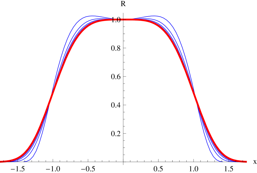
Figure 1: $R_{p,q}\left(n,\,n/2,\,x\,n^{3/4}\right)$ (blue curves) versus $x$ at $z=-9$ and $y=2\,w=-0.105391$ for $n=2^{6}$, $2^{8}$, $2^{10}$ and $2^{12}$. The red curve is the asymptote $e^{-0.719718\,x^{4}}$.

VI.2 Wide and double-peaked distributions

Changing $p$ only slightly, say on the order of $1/n^{3/2}$, allows us to move around in the region where the distribution is wide. The end result is that with $q=1+z/n$ and $p=1+2\,w/n+a/n^{3/2}$ we get

$$R_{p,q}\left(n,\,n/2,\,x\,n^{3/4}\right)\sim\exp\left(\frac{w\,z\,(2\,w+z)\,x^{4}}{6}+\frac{a\,z\,(1+w)\,x^{2}}{2\,w-z}\right)$$ (63)

The ratio expression gets nicer if we change the coefficient of $1/n^{3/2}$. We suggest the following parametrization instead; with $q=1+z/n$ let

$$p=1+\frac{2\,w}{n}+\frac{a\,w\,\left(z^{2}-4\,w^{2}\right)}{3\,(1+w)\,n^{3/2}}$$ (64)

and we receive

$$R_{p,q}\left(n,\,n/2,\,x\,n^{3/4}\right)\sim\exp\left(\frac{w\,z\,(2\,w+z)}{6}\,\left(x^{4}-2\,a\,x^{2}\right)\right)$$ (65)

This puts the maximum at $x=\pm\sqrt{a}$ for $a>0$ and at $x=0$ for $a\leq 0$.

Figure 2 works like figure 1 but here with the parameter $a$ set to $1$. It shows $R_{p,q}\left(n,\,n/2,\,x\,n^{3/4}\right)$ for $z=-9$ with $p=1-0.105391/n-1.50171/n^{3/2}$ and the asymptotic ratio is given by (65), that is, $e^{-0.719718\,(x^{4}-2\,x^{2})}$. The red curve is the asymptote and the blue curves are for finite $n$ where the larger $n$ are closer to the asymptote. Had we set $a<0$ the distributions would still be wide but with a single peak in the middle.

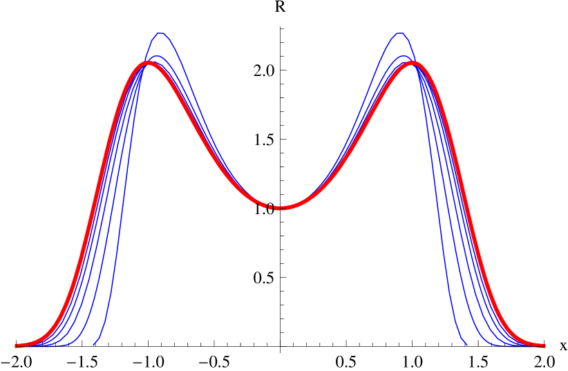
Figure 2: $R_{p,q}\left(n,\,n/2,\,x\,n^{3/4}\right)$ (blue curves) versus $x$ at $z=-9$ and $a=1$ so that $q=1-9/n$ and $p=1-0.105391/n-1.50171/n^{3/2}$ for $n=2^{6}$, $2^{8}$, $2^{10}$, $2^{12}$ and $2^{14}$. The red curve is the asymptote $e^{-0.719718\,(x^{4}-2\,x^{2})}$.

VI.3 Peakish distributions

If we instead choose a middle ratio of $1+a/n$ then we receive a sharply peaked distribution. Say that we want

$$R_{p,q}\left(n,\,n/2,\,1\right)=\frac{p^{n/2}-q^{n/2}}{p^{n/2+1}-q^{n/2+1}}=1+\frac{a}{n}$$ (66)

for $p=1+y_{1}/n+\cdots$ and $q=1+z/n$ as before. Note that $a=-2$ corresponds to a binomial distribution, so we are usually interested in the case $-2<a<0$. After expanding the equation we receive as before, from the first term of the left and right hand side, the equation

$$(a+y_{1})\,e^{y_{1}/2}=(a+z)\,e^{z/2}$$ (67)

which has the solution $y_{1}=2\,w-a$ where

$$w=\mathrm{W}\left(\frac{a+z}{2}\,e^{(a+z)/2}\right)$$ (68)

The second equation, which is slightly longer, has the solution

$$y_{2}=\frac{(a-2\,w+z)\,\left(a^{2}\,(w+2)-2\,a\,w^{2}-w\,z\,(2\,w+z)\right)}{2\,(w+1)\,(a+z)}$$ (69)

but we do not really need it at this moment. This gives a distribution with a width of the order $\sqrt{n}$. Computing the limit ratio gives us

$$R_{p,q}\left(n,\,n/2,\,x\,\sqrt{n}\right)\sim e^{a\,x^{2}}$$ (70)

thus giving us an essentially gaussian distribution. Note that it does not depend on $z$ in its current form. Of course, we expect other terms to depend on $z$ but these vanish when $n\to\infty$.

VI.4 Two separate peaks

Suppose that we want the peaks located outside the middle. Defining $k=\frac{n}{2}\,(1+\mu)$ for $0<\left\lvert\mu\right\rvert<1$ means that we move the peaks out from the middle and that we move to another isocurve. We keep $q=1+z/n$ and $p=1+y_{1}/n+y_{2}/n^{2}+\cdots$ and solve $R_{p,q}\left(n,\,k,\,1\right)=1$, i.e.

$$p^{n-k+1}-p^{k}=q^{n-k+1}-q^{k}$$ (71)

With $k=\frac{n}{2}\,(1+\mu)$ we use (35) on both sides and find the equation

$$\exp\left(\frac{y_{1}}{2}\,(1-\mu)\right)-\exp\left(\frac{y_{1}}{2}\,(1+\mu)\right)=\exp\left(\frac{z}{2}\,(1-\mu)\right)-\exp\left(\frac{z}{2}\,(1+\mu)\right)$$ (72)

which we rewrite as

$$e^{y_{1}/2}\,\sinh{\frac{\mu\,y_{1}}{2}}=e^{z/2}\,\sinh{\frac{\mu\,z}{2}}$$ (73)

At this point it would be appropriate to define the function $s=\mathrm{\Omega}_{\mu}\left(x\right)$, for $0<\mu<1$, as the maximum solution to the equation

$$x=e^{s}\,\sinh\left(s\,\mu\right)$$ (74)

Note here that the function $e^{x}\,\sinh(\mu\,x)$ has a minimum at $(-\operatorname{atanh}\mu)/\mu$ for $0<\mu<1$ and, due to symmetry, a maximum at the same point for $-1<\mu<0$. The function $\Omega$ returns a value in the interval

$$-\frac{\operatorname{atanh}{\mu}}{\mu}<s<0$$ (75)

The solution sought in our equation is thus $y_{1}=2\,w$ where

$$w=\mathrm{\Omega}_{\mu}\left(e^{z/2}\,\sinh\frac{\mu\,z}{2}\right)$$ (76)

We should mention that $\mathrm{\Omega}_{\mu}\left(x\right)$ is a natural extension of $\mathrm{W}\left(x\right)$. In fact, if we let $w=\mathrm{W}\left(x\,e^{x}\right)$ then

$$\mathrm{\Omega}_{\mu}\left(e^{x}\,\sinh\mu\,x\right)=w+\frac{w\,(x^{2}-w^{2})}{6\,(1+w)}\,\mu^{2}+\cdots$$ (77)

giving a good approximation for small values of $\mu$. The reader may recall (60) above for comparison.

Having computed $p=1+y_{1}/n$ we compute the upper and lower bounds of the ratio as before. Unfortunately, the ratio has the rather ghastly expression

$$R_{p,q}\left(n,\,\frac{n}{2}\,(1+\mu),\,x\,\sqrt{n}\right)\sim\\ \exp\left\{\frac{x^{2}}{2}\,\left(2\,w+z-\frac{e^{\mu w+\frac{\mu z}{2}}\left(e^{2w}-e^{z}\right)(z-2w)}{-e^{2\mu w+w+\frac{z}{2}}+e^{\mu w+2w+\frac{\mu z}{2}}+e^{\mu w+\frac{\mu z}{2}+z}-e^{w+\mu z+\frac{z}{2}}}\right)\right\}$$ (78)

where $w$ is defined by (76).

In figure 3 we show how the finite cases approach their asymptote for $\mu=1/3$ and $z=-9$. This gives $p=1-0.153208/n$ and the asymptotic ratio is given by (78), that is, $e^{-0.103551\,x^{2}}$. The red curve is the asymptote and the blue curves are for finite $n$ where the larger $n$ are closer to the asymptote.

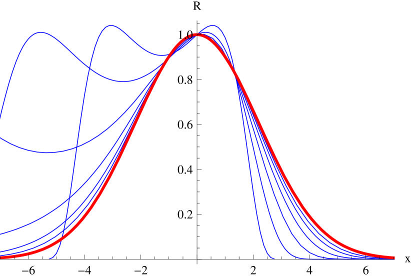
Figure 3: $R_{p,q}\left(n,\,n/2\,(1+\mu),\,x\,\sqrt{n}\right)$ (blue curves) versus $x$ at $\mu=1/3$ and $z=-9$ so that $q=1-9/n$ and $p=1-0.153208/n$ for $n=2^{6}$, $2^{8}$, $2^{10}$, $2^{12}$, $2^{14}$ and $2^{16}$. The red curve is the asymptote $e^{-0.103551\,x^{2}}$.

VII Moving along a diagonal

With $q=1+z/n$ and using the expressions given by (64) and (65), we can move around in the region where $R_{p,q}\left(n,\,n/2,\,1\right)$ is very close to $1$. It is understood here that a change in the parameter $a$ only changes $p$, i.e. we only move in the $p$-direction and keep $q$ fixed. Let us instead say that we want to move, ever so slightly, in both the $p$- and $q$-direction. If the movement is on the order $1/n^{3/2}$ we can translate it to a different parameter $a$ in the expression given by (64).

Given a $z$ in $q=1+z/n$ the starting point for $p$ is $p=1+y/n$ with $y=2\,w$ and $w$ given by (59). Let us think of the starting coordinate as $(y_{0},\,z_{0})$. We wish to move from this point $s/\sqrt{n}$ steps in the direction $t$, where the limit $t\to\infty$ corresponds to the case where we only move in the direction $y$ (or $p$). The new point is now

$$(y_{1},\,z_{1})=\left(y_{0}+\frac{s\,t}{\sqrt{1+t^{2}}\,\sqrt{n}},\,z_{0}+\frac{s}{\sqrt{1+t^{2}}\,\sqrt{n}}\right)$$ (79)

and note here that $\sqrt{(y_{1}-y_{0})^{2}+(z_{1}-z_{0})^{2}}=\left\lvert s\right\rvert/\sqrt{n}$.

Having moved in the $z$-direction from $z_{0}$ to $z_{1}$ we now compute the point $y_{2}$ so that $(y_{2},\,z_{1})$ stays on the isocurve with $R_{p,q}\left(n,\,n/2,\,1\right)=1$. A small change in $z$ requires only a small change in $y$ to preserve this property.

With $w_{0}=\mathrm{W}\left(z_{0}\,e^{z_{0}/2}/2\right)$ we have the series expansion

$$\mathrm{W}\left(\frac{(z_{0}+x)\,\exp\left((z_{0}+x)/2\right)}{2}\right)=w_{0}+\frac{x\,w_{0}\,(z_{0}+2)}{2\,z_{0}\,(w_{0}+1)}+\cdots$$ (80)

giving an approximation for small $x$. We want to set

$$x=\frac{s}{\sqrt{1+t^{2}}\,\sqrt{n}}$$ (81)

and thus we have

$$y_{2}=y_{0}+\frac{s\,w_{0}\,(z_{0}+2)}{z_{0}\,(w_{0}+1)\,\sqrt{1+t^{2}}\,\sqrt{n}}$$ (82)

The difference $y_{1}-y_{2}$ is what we want:

$$y_{1}-y_{2}=\frac{s\,t}{\sqrt{1+t^{2}}\,\sqrt{n}}-\frac{s\,w_{0}\,(z_{0}+2)}{z_{0}\,(w_{0}+1)\,\sqrt{1+t^{2}}\,\sqrt{n}}=$$ (83)

$$\frac{s}{\sqrt{1+t^{2}}\,\sqrt{n}}\,\left(t-\frac{w_{0}\,(z_{0}+2)}{z_{0}\,(w_{0}+1)}\right)$$ (84)

Now solve

$$y_{1}-y_{2}=\frac{a\,w_{0}\,(z_{0}^{2}-4\,w_{0}^{2})}{3\,(w_{0}+1)\,\sqrt{n}}$$ (85)

where the right hand side is extracted from (64). This gives

$$a=\frac{3\,s}{\sqrt{1+t^{2}}}\,\frac{t\,z_{0}\,(w_{0}+1)-w_{0}\,(z_{0}+2)}{z_{0}\,w_{0}\,(z_{0}^{2}-4\,w_{0}^{2})}$$ (86)

which then gives the ratio in (65).

As an example, we take the case $p=q$ which corresponds to $t=1$ and $z_{0}\to-2^{-}$. Taking the limit of the expression for $a$ gives

$$\lim_{z\to-2^{-}}a=-\frac{3\,s}{8\,\sqrt{2}}$$ (87)

which corresponds to the coefficient ratio

$$R_{p,q}\left(n,\,n/2,\,x\,n^{3/4}\right)\sim\exp\left(-\frac{4}{3}\,(x^{4}-2\,a\,x^{2})\right)=\exp\left(-\frac{4}{3}\,x^{4}-\frac{s}{\sqrt{2}}\,x^{2}\right)$$ (88)

Compare this with lemma IV.6; the parameter $a$ in the lemma corresponds to taking $s=a\,\sqrt{2}$ steps in direction $t=1$ and this gives the same coefficient ratio as in the lemma.

VIII Moments

Once we have the ratios (62), (65), (70), (78) it is an easy task to compute moments of the distributions. Let us do this for the most interesting case of (65). First, to make the notation somewhat simpler, denote $\phi=\mathrm{\Phi}\!\left(z\right)=-w\,z\,(2\,w+z)/6$, i.e. $\phi>0$, with $w$ as in (59), so that

$$R_{p,q}\left(n,\,n/2,\,x\,n^{3/4}\right)\sim e^{-\phi\,(x^{4}-2\,a\,x^{2})}$$ (89)

where $a$ is defined by (64). We use the notation

$$\sigma_{m}=\left\langle\left\lvert k-\frac{n}{2}\right\rvert^{m}\right\rangle$$ (90)

for the $m$th moment of the probability distribution of $k=0,\ldots,n$. Define also

$$\varrho_{m}=\int\limits_{-\infty}^{+\infty}\left\lvert x\right\rvert^{m}\,\exp\left(-\phi\,(x^{4}-2\,a\,x^{2})\right)\,\mathrm{d}x,\quad m\geq 0$$ (91)

so that the $m$th moment becomes $\left\langle\left\lvert x\right\rvert^{m}\right\rangle=\varrho_{m}/\varrho_{0}$. For $m=0$ we have

$$\varrho_{0}=\,\left\{\begin{array}[]{ll}\Big{.}\frac{\pi\,\sqrt{a}}{2}\,\exp\left(\phi\,a^{2}/2\right)\,\left(I_{1/4}\left(\scriptstyle\phi\,a^{2}/2\right)+I_{-1/4}\left(\scriptstyle\phi\,a^{2}/2\right)\right),&\textrm{for $a>0$}\\ \Big{.}\frac{\sqrt{-a}}{\sqrt{2}}\,\exp\left(\phi\,a^{2}/2\right)\,K_{1/4}\left(\scriptstyle\phi\,a^{2}/2\right),&\textrm{for $a<0$}\\ \Big{.}\frac{\Gamma\!\left(\scriptstyle 1/4\right)}{2\,\phi^{1/4}},&\textrm{for $a=0$}\end{array}\right.$$ (92)

so that

$$1=\sum_{k=-n/2}^{n/2}\mathbb{P}_{p,q}\left(n,\,n/2+k\right)\sim n^{3/4}\,\mathbb{P}_{p,q}\left(n,\,n/2\right)\,\varrho_{0}$$ (93)

Next, for $m=1$

$$\varrho_{1}=\frac{\sqrt{\pi}}{2\,\sqrt{\phi}}\,\exp\left(\phi\,a^{2}\right)\,\left(1+\mathrm{erf}\left(a\,\sqrt{\phi}\right)\right)$$ (94)

where $-1<\mathrm{erf}\left(x\right)<1$ is the error function. and thus

$$\sigma_{1}=\left\langle\left\lvert k-\frac{n}{2}\right\rvert\right\rangle\sim n^{3/4}\,\frac{\varrho_{1}}{\varrho_{0}}$$ (95)

In general we have for $m\geq 0$ that

$$\sigma_{m}=\left\langle\left\lvert k-\frac{n}{2}\right\rvert^{m}\right\rangle\sim n^{3\,m/4}\,\frac{\varrho_{m}}{\varrho_{0}}$$ (96)

where $\varrho_{m}$ is given by

$$\left\{\begin{array}[]{ll}\Big{.}\!\!\!\frac{\phi^{-(m+1)/4}}{2}\,\left(\Gamma\!\left(\scriptstyle\frac{m+1}{4}\right)\,{}_{1}\mathrm{F}_{1}\!\left(\scriptstyle\frac{m+1}{4},\,\frac{1}{2},\,\phi\,a^{2}\right)+2\,a\,\sqrt{\phi}\,\Gamma\!\left(\scriptstyle\frac{m+3}{4}\right)\,{}_{1}\mathrm{F}_{1}\!\left(\scriptstyle\frac{m+3}{4},\,\frac{3}{2},\,\phi\,a^{2}\right)\right),&a>0\\ \Big{.}\!\!\!\frac{\phi^{-(m+1)/4}}{2^{(m+1)/2}}\,\Gamma\!\left(\scriptstyle\frac{m+1}{2}\right)\,\mathrm{U}\!\left(\scriptstyle\frac{m+1}{4},\,\frac{1}{2},\,\phi\,a^{2}\right),&a<0\\ \Big{.}\!\!\!\frac{\phi^{-(m+1)/4}}{2}\,\Gamma\!\left(\scriptstyle\frac{m+1}{4}\right),&a=0\\ \end{array}\right.$$ (97)

Here ${}_{1}\mathrm{F}_{1}\!\left(\scriptstyle a,\,b,\,c\right)$ and $\mathrm{U}\!\left(\scriptstyle a,\,b,\,c\right)$ denote the confluent hypergeometric functions of the first and second kind respectively. If we want to compute cumulant ratios we first need moment ratios which of course is easy now. For example, in the case of $a=0$ we have

$$\frac{\sigma_{2}}{\sigma_{1}^{2}}\sim \frac{\varrho_{0}\,\varrho_{2}}{\varrho_{1}^{2}}=\sqrt{2}=1.4142\ldots$$ (98)

$$\frac{\sigma_{4}}{\sigma_{2}^{2}}\sim \frac{\varrho_{0}\,\varrho_{4}}{\varrho_{2}^{2}}=\frac{\Gamma\!\left(\scriptstyle 1/4\right)^{4}}{8\,\pi^{2}}=2.1884\ldots$$ (99)

$$\frac{\sigma_{6}}{\sigma_{2}^{3}}\sim \frac{\varrho_{0}^{2}\,\varrho_{6}}{\varrho_{2}^{3}}=\frac{3\,\Gamma\!\left(\scriptstyle 1/4\right)^{4}}{8\,\pi^{2}}=6.5653\ldots$$ (100)

These moment ratios are the same as obtained in the 5-dimensional Ising model, see e.g. Brezin and Zinn-Justin (1985).

IX Fine-tuning the exponents

Note (65) and, as before, keep $\mathrm{\Phi}\!\left(z\right)=-w\,z\,(2\,w+z)/6$ where $w$ is defined by (59). Recall that the first and second absolute moments obtained from (97) for $a=0$ are

$$\sigma_{1} \sim n^{3/4}\,\frac{\varrho_{1}}{\varrho_{0}}=n^{3/4}\,\frac{\sqrt{\pi}}{\Gamma\!\left(\scriptstyle 1/4\right)}\,\frac{1}{\mathrm{\Phi}\!\left(z\right)^{1/4}}\propto\frac{n^{3/4}}{\mathrm{\Phi}\!\left(z\right)^{1/4}}$$ (101)

$$\sigma_{2} \sim n^{3/2}\,\frac{\varrho_{2}}{\varrho_{0}}=n^{3/2}\,\frac{\pi\,\sqrt{2}}{\Gamma\!\left(\scriptstyle 1/4\right)^{2}}\,\frac{1}{\sqrt{\mathrm{\Phi}\!\left(z\right)}}\propto\frac{n^{3/2}}{\sqrt{\mathrm{\Phi}\!\left(z\right)}}$$ (102)

The argument $z$ is allowed to depend on $n$ but probably not to a high order. At this point it is not clear how $z$ may depend on $n$ for the calculations leading to (65) and $\mathrm{\Phi}\!\left(z\right)$ to work. We will assume, for the moment (see the end of this section), that the expressions for the moments of (97) are valid when $z=\mathcal{O}\left(\log n\right)$.

The series expansion of $\mathrm{W}\left(x\right)$ is

$$w=\mathrm{W}\left(x\right)=x-x^{2}+\frac{3\,x^{3}}{2}-\frac{8\,x^{4}}{3}+\cdots$$ (103)

With $x=e^{z/2}\,z/2$, and note that $z$ is negative, we have

$$w=\mathrm{W}\left(x\right)=\mathrm{W}\left(\frac{z\,e^{z/2}}{2}\right)=\frac{z\,e^{z/2}}{2}-\frac{z^{2}\,e^{z}}{4}+\frac{3\,z^{3}\,e^{3\,z/2}}{16}+\cdots$$ (104)

so that

$$\mathrm{\Phi}\!\left(z\right)=\frac{-z\,w\,(2\,w+z)}{6}=-\frac{z^{3}\,e^{z/2}}{12}-\frac{z^{3}\,e^{z}}{12}+\frac{z^{4}\,e^{z}}{24}+\cdots$$ (105)

Set $z=\lambda_{0}+\lambda_{1}\,\log n+\lambda_{2}\,\log\log n+\lambda_{3}\,\log\log\log n$ with $\lambda_{1},\lambda_{2}\leq 0$ and focus on the first term of (105).

$$\mathrm{\Phi}\!\left(z\right)\sim\frac{-1}{12}\,\left(\lambda_{0}+\lambda_{1}\,\log n+\lambda_{2}\,\log\log n+\lambda_{3}\,\log\log\log n\right)^{3}\\ e^{\lambda_{0}/2}\,n^{\lambda_{1}/2}\,\log^{\lambda_{2}/2}n\,\left(\log\log n\right)^{\lambda_{3}/2}$$ (106)

We are interested in two special cases. First choose $\lambda_{1}<0$, $\lambda_{2}=-6$ and $\lambda_{3}=0$. This gives

$$\mathrm{\Phi}\!\left(z\right)\sim\frac{(-\lambda_{1})^{3}}{12}\,e^{\lambda_{0}/2}\,n^{\lambda_{1}/2}$$ (107)

Combining this with (101) we receive

$$\sigma_{1}\sim\frac{3^{1/4}\,\sqrt{2\,\pi}}{\Gamma\!\left(\scriptstyle 1/4\right)}\,\frac{n^{3/4-\lambda_{1}/8}}{(-\lambda_{1})^{3/4}\,e^{\lambda_{0}/8}}$$ (108)

and

$$\sigma_{2}\sim\frac{2\,\sqrt{6}\,\pi}{\Gamma\!\left(\scriptstyle 1/4\right)^{2}}\,\frac{n^{3/2-\lambda_{1}/4}}{(-\lambda_{1})^{3/2}\,e^{\lambda_{0}/4}}$$ (109)

Had we let $\lambda_{2}=0$, instead of $\lambda_{2}=-6$, then we would have ended up with a factor $\log^{3/4}n$ in the denominator of (108) and a factor $\log^{3/2}n$ in the denominator of (109). For the second case we choose $\lambda_{1}=0$, $\lambda_{2}<0$ and $\lambda_{3}=-6$. We get

$$\mathrm{\Phi}\!\left(z\right)\sim\frac{(-\lambda_{2})^{3}}{12}\,e^{\lambda_{0}/2}\,\log^{\lambda_{2}/2}n$$ (110)

This together with (101) gives us

$$\sigma_{1}\sim\frac{3^{1/4}\,\sqrt{2\,\pi}}{\Gamma\!\left(\scriptstyle 1/4\right)}\,\frac{n^{3/4}\,\log^{-\lambda_{2}/8}n}{(-\lambda_{2})^{3/4}\,e^{\lambda_{0}/8}}$$ (111)

and

$$\sigma_{2}\sim\frac{2\,\sqrt{6}\,\pi}{\Gamma\!\left(\scriptstyle 1/4\right)^{2}}\,\frac{n^{3/2}\,\log^{-\lambda_{2}/4}n}{(-\lambda_{2})^{3/2}\,e^{\lambda_{0}/4}}$$ (112)

These expressions obviously converge extremely slowly and are probably not of any use for $n$ that might occur in practical situations.

We have managed to verify (108) and (109) by using the method described in section VI, again using Mathematica, only in the special case $z=-\log n$, i.e. $\lambda_{1}=-1$, $\lambda_{0}=\lambda_{2}=\lambda_{3}=0$. We could then confirm that

$$R_{p,q}\left(n,\,n/2,\,\frac{x\,n^{7/8}}{\log^{3/4}n}\right)\sim\exp\left(\frac{-x^{4}}{12}\right)$$ (113)

Computing the moments of this distribution produces the same result as setting $\lambda_{1}=-1$ and $\lambda_{0}=\lambda_{2}=\lambda_{3}=0$ in (106) and then computing the moments in the same the way we obtained (108) and (109). A more general computation seems not to be within reach with our current set of tools though. To conclude this section we note that the exponent of $n$ in (113) is $3/4-\lambda_{1}/8$. For this exponent to stay less than one we thus need $\lambda_{1}>-2$, giving us a bound on $z$.

X The Ising model

A state $\tau$ on a graph $G$ is a function from the set of vertices to $\{\pm 1\}$. There are thus $2^{n}$ states for a graph on $n$ vertices. We define the energy of a state as $E(\tau)=\sum_{ij}\tau_{i}\tau_{j}$ where the sum is taken over all edges $ij$ of $G$. The magnetisation is defined as $M(\tau)=\sum_{i}\tau_{i}$ with the sum taken over all vertices $i$ of $G$. Note that $-n\leq M\leq n$ and it only takes every alternate value, i.e. $M\in\{-n,-n+2,-n+4,\ldots,n-4,n-2,n\}$. We will often need to refer to it in terms of how many negative spins the state has. If $k$ spins are negative then $M=n-2\,k$.

The partition function of the Ising model is defined for any graph $G$ as

$$\mathrm{Z}(G;\,x,\,y)=\sum_{\tau}x^{E(\tau)}\,y^{M(\tau)}=\sum_{E,M}a(E,M)\,x^{E}\,y^{M}$$ (114)

The coefficients $a(E,M)$ then are defined as the number of states with energy $E$ and magnetisation $M$. Denote the number of states at energy $E$ by $a(E)=\sum_{M}a(E,M)$. Note that the number of states at magnetisation $M$ is just $\binom{n}{k}$, where $k=(n-M)/2$ is the number of negative spins. Let also $\mathrm{Z}_{k}$ denote the terms of $\mathrm{Z}$ with magnetisation $M=n-2\,k$ for a graph on $n$ vertices, so that $\mathrm{Z}=\mathrm{Z}_{0}+\mathrm{Z}_{2}+\cdots+\mathrm{Z}_{n}$, i.e. $\mathrm{Z}_{k}$ are the terms corresponding to $k$ negative spins.

If we evaluate the partition function in $x=e^{K}$ and $y=e^{H}$ with $K$ the dimensionless coupling, or inverse temperature $J/k_{B}T$, and $H=h/k_{B}T$ as the dimensionless external magnetic field, we obtain the physical partition function denoted $\mathcal{Z}=\mathcal{Z}(G;\,K,\,H)=\mathrm{Z}(G;\,e^{K},\,e^{H})$, though we are usually interested only in the case when $H=0$ (or $y=1$). Analogously, we write $\mathcal{Z}=\mathcal{Z}_{0}+\cdots+\mathcal{Z}_{n}$. The dimensionless and normalised free energy is defined as $\mathcal{F}=\left(\log\mathcal{Z}\right)/n$. From the derivatives of the free energy we can now obtain other physical quantities such as the internal energy $\partial\mathcal{F}/\partial K$ and the specific heat $\partial^{2}\mathcal{F}/\partial K^{2}$ though we shall not be needing the latter for this investigation.

We assume the Boltzmann distribution on the states so that (with $H=0$) the probability for state $\tau$ is

$$\mathbb{P}\left(\tau\right)=\frac{e^{K\,E(\tau)}}{\mathcal{Z}}$$ (115)

We have then especially that the probability for energy $E$ is

$$\mathbb{P}\left(E\right)=\frac{a(E)\,e^{K\,E}}{\mathcal{Z}}$$ (116)

and the probability for magnetisation $M$ is

$$\mathbb{P}\left(M\right)=\frac{1}{\mathcal{Z}}\,\sum_{E}a(E,M)\,e^{K\,E}=\frac{\mathcal{Z}_{k}}{\mathcal{Z}}$$ (117)

where $M=n-2\,k$.

Denote by $K^{*}$ the coupling where $\mathcal{Z}_{n/2-1}=\mathcal{Z}_{n/2}=\mathcal{Z}_{n/2+1}$. This coupling will correspond to the relation $R_{p,q}\left(n,\,n/2,\,1\right)=1$ for some choice of $p,q$. We define the (spontaneous) normalised magnetisation $\bar{\mu}=\left\langle\left\lvert M\right\rvert\right\rangle/n$ and the (spontaneous) susceptibility $\bar{\chi}=\mathrm{Var}\left(\left\lvert M\right\rvert\right)/n=\left(\left\langle M^{2}\right\rangle-\left\langle\left\lvert M\right\rvert\right\rangle^{2}\right)/n$. The pure susceptibility is simply $\chi=\mathrm{Var}\left(M\right)/n=\left\langle M^{2}\right\rangle=4\,\sigma_{2}/n$. Since $M=n-2\,k$ we thus have $\bar{\mu}=2\,\sigma_{1}/n$ and $\bar{\chi}=4\,(\sigma_{2}-\sigma_{1}^{2})/n$. Recall the traditional finite-size scaling laws which claim that in the critical region, i.e. near $K_{c}$, $\bar{\mu}\propto L^{-\beta/\nu}$ and $\bar{\chi}\propto L^{\gamma/\nu}$. Being near $K_{c}$ means that $\left\lvert K-K_{c}\right\rvert\propto L^{-1/\nu}$ and we especially expect $K^{*}$ to belong to this region. Though the high- and low-temperature exponents may or may not be equal for three dimensions, see Häggkvist et al. (2007) for an in-depth numerical investigation of this matter, the details of these exponents are not important for our present investigation. What matters is that there are exponents that guide the growth of e.g. the susceptibility near $K_{c}$.

X.1 The complete graph

For a complete graph, denoted $K_{n}$ on $n$ vertices and $\binom{n}{2}$ edges the partition function is easy to compute. Suppose $k$ of the vertices are assigned spin $-1$ and the other $n-k$ have spin $+1$. The magnetisation is obviously $M=n-2\,k$ and the energy is

$$E=\binom{k}{2}+\binom{n-k}{2}-k\,(n-k)=\binom{n}{2}-2\,k\,(n-k)$$ (118)

The partition function is then

$$\mathrm{Z}(K_{n};\,x,\,y)=x^{\binom{n}{2}}\,y^{n}\,\sum_{k=0}^{n}\binom{n}{k}\,\left(\frac{1}{x^{2}}\right)^{k\,(n-k)}\,\left(\frac{1}{y^{2}}\right)^{k}$$ (119)

and with $y=1$ we have

$$\mathrm{Z}(K_{n};\,x,\,1)=x^{\binom{n}{2}}\,\sum_{k=0}^{n}\genfrac{[}{]}{0.0pt}{0}{n}{k}_{q,q}=x^{\binom{n}{2}}\,\Psi_{q,q}\left(n\right)$$ (120)

where $q=1/x^{2}$. Thus we have

$$\mathcal{Z}(K_{n};\,K,\,0)=\exp\left\{K\,\binom{n}{2}\right\}\,\Psi_{q,q}\left(n\right)$$ (121)

where $q=\exp(-2\,K)$. Obviously we have

$$\mathbb{P}\left(M=n-2\,k\right)=\mathbb{P}_{q,q}\left(n,\,k\right)$$ (122)

Since we have defined the critical temperature as the $K=K^{*}$ where the middle ratio is $1$, i.e. $\mathbb{P}\left(M=-2\right)=\mathbb{P}\left(M=0\right)=\mathbb{P}\left(M=+2\right)$ then this corresponds to the point where $R_{q,q}\left(n,\,n/2,\,1\right)=1$, which takes place at $q=n/(n+2)$ as we saw in lemma IV.1. Thus $K^{*}=\frac{1}{2}\,\log\left(1+\frac{2}{n}\right)$ for $K_{n}$.

In short, the partition function and the magnetisation distribution for $K_{n}$ can be expressed in terms of $p,q$-binomial coefficients. Does this hold for all graphs? No. In fact, it seems to only be true for $K_{n}$. However, it does seem to hold asymptotically as the order of the graphs increase, for some interesting classes of graphs. The precise formulation of such a statement remains and falls outside this paper.

X.2 The average graph

Let us compute the sum of all partition functions taken over all graphs on $n$ vertices.

$$\bar{\mathrm{Z}}_{n}(x,y)=\sum_{G\subseteq K_{n}}\mathrm{Z}(G;\,x,\,y)=$$ (123)

$$\sum_{i=0}^{n}\binom{n}{i}\,y^{n-2\,i}\,\sum_{j=0}^{\binom{i}{2}}\binom{\binom{i}{2}}{j}\,x^{j}\,\sum_{k=0}^{\binom{n-i}{2}}\binom{\binom{n-i}{2}}{k}\,x^{k}\,\sum_{\ell=0}^{i\,(n-i)}\binom{i\,(n-i)}{\ell}\,x^{-\ell}=$$ (124)

$$\sum_{i=0}^{n}\binom{n}{i}\,y^{n-2\,i}\,\left(1+x\right)^{\binom{i}{2}}\,\left(1+x\right)^{\binom{n-i}{2}}\,\left(1+\frac{1}{x}\right)^{\binom{i\,(n-i)}{2}}=$$ (125)

$$\left(1+x\right)^{\binom{n}{2}}\,y^{n}\,\sum_{i=0}^{n}\binom{n}{i}\,\left(\frac{1}{y^{2}}\right)^{i}\,\left(\frac{1}{x}\right)^{i\,(n-i)}$$ (126)

and for $y=1$ we have

$$\bar{\mathrm{Z}}_{n}(x,1)=\left(1+x\right)^{\binom{n}{2}}\,\sum_{i=0}^{n}\binom{n}{i}\,\left(\frac{1}{x}\right)^{i\,(n-i)}=$$ (127)

$$\left(1+x\right)^{\binom{n}{2}}\,\sum_{i=0}^{n}\genfrac{[}{]}{0.0pt}{0}{n}{i}_{q,q}=\left(1+x\right)^{\binom{n}{2}}\,\Psi_{q,q}\left(n\right)$$ (128)

where $q=1/x$ so that $K^{*}=\log(1+2/n)$. Again we have $\mathbb{P}\left(M=n-2\,k\right)=\mathbb{P}_{q,q}\left(n,\,k\right)$. The mean magnetisation distribution can then be modelled by $p,q$-binomial coefficients, though with $p=q$, just as for the complete graph.

X.3 The complete bipartite graph

What about $K_{u,v}$, i.e. the complete bipartite graph on $n=u+v$ vertices? Now the partition function is

$$\mathrm{Z}(K_{u,v};\,x,\,y)=$$ (129)

$$\sum_{i=0}^{u}\sum_{j=0}^{v}\binom{u}{i}\,\binom{v}{j}\,y^{u+v-2\,i-2\,j}\,x^{i\,j+(u-i)\,(v-j)-i\,(v-j)-j\,(u-i)}=$$ (130)

$$x^{u\,v}\,y^{u+v}\,\sum_{i=0}^{u}\sum_{j=0}^{v}\binom{u}{i}\,\binom{v}{j}\,\left(\frac{1}{y^{2}}\right)^{i+j}\,\left(\frac{1}{x^{2}}\right)^{i\,(v-j)+j\,(u-i)}$$ (131)

which for $y=1$ gives us

$$\mathrm{Z}(K_{u,v};\,x,\,1)=$$ (132)

$$x^{u\,v}\,\sum_{i=0}^{u}\sum_{j=0}^{v}\binom{u}{i}\,\binom{v}{j}\,\left(\frac{1}{x^{2}}\right)^{i\,(v-j)+j\,(u-i)}=$$ (133)

$$\sum_{k=0}^{u+v}\sum_{\ell}\binom{u}{\ell}\,\binom{v}{k-\ell}\,x^{(u-2\,\ell)\,(v-2\,(k-\ell))}$$ (134)

which defines the partial sums for $y=1$ as

$$\mathrm{Z}_{k}=\sum_{\ell}\binom{u}{\ell}\,\binom{v}{k-\ell}\,x^{(u-2\,\ell)\,(v-2\,(k-\ell))}$$ (135)

Data suggests that

$$\mathbb{P}\left(M=n-2\,k\right)=\frac{\mathcal{Z}_{k}}{\mathcal{Z}}\approx\mathbb{P}_{p,q}\left(n,\,k\right)$$ (136)

given an appropriate choice of $p$ and $q$ and for a rather wide range of temperatures. It does however not seem to hold if $u$ differ from $v$. In the left panel of figure 4 we show a sample of magnetisation distributions together with fitted $p,q$-distributions for a $K_{32,32}$. To find the appropriate $p$ and $q$ we used the method described in the $p,q$-find algorithm in section III. The fit is excellent. The right panel of figure 4 shows $y=n\,(p-1)$ versus $z=n\,(q-1)$ for a range of temperatures and for complete bipartite graphs of different sizes. High temperatures, $K=0$ gives $p=q=1$, i.e. $y=z=0$ in the upper right corner. As the temperature decreases, i.e. with increasing $K$, we move along the curves. The points are where the distribution is exactly flat, i.e. the inverse temperature $K^{*}$ where the middle probabilities are equal. We have no exact closed form expression for $K^{*}$ but one can show that the series expansion of this inverse temperature for $K_{n/2,n/2}$, i.e. a total of $n$ vertices is

$$K^{*}=\frac{2}{n}-\frac{3}{n^{2}}+\frac{11}{3\,n^{3}}-\frac{101}{24\,n^{4}}+\frac{3827}{480\,n^{5}}+\cdots$$ (137)

The calculations behind this are rather long and were done with Mathematica. Compare this with the expansion in the previous subsection for the complete graph on $n$ vertices, $K_{n}$, which begins $K^{*}=1/n-1/n^{2}+4/3n^{3}+\cdots$. In the lower left corner the distribution has $\mathbb{P}\left(M=n\right)=\mathbb{P}\left(M=n-2\right)$, i.e. at $K=\log{n}/n$.

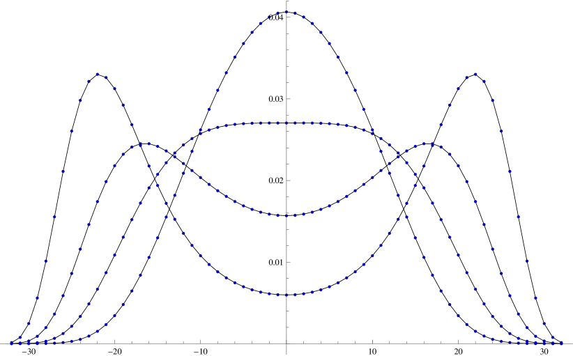
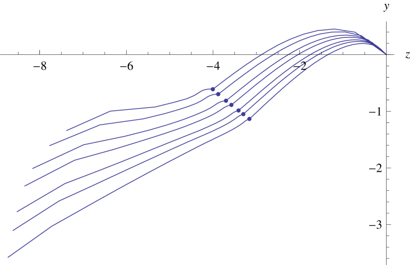
Figure 4: Left: magnetisation distributions for $K_{32,32}$ (points) and fitted $\mathbb{P}_{p,q}\left(64,\,k\right)$ (lines) vs $k-32$ for four different temperatures. Right: $y=n\,(p-1)$ versus $z=n\,(q-1)$ for $K_{n/2,n/2}$, with $n=24,32,48,64,96,128,192$ (downwards). Points represent $K^{*}$. Low temperatures in lower left corner.

The points in the right panel of figure 4 should approach $z=y=-2$. One can show that the distribution of a balanced bipartite graph $K_{n/2,n/2}$ has the shape

$$R\left(n,\,n/2,\,x\,n^{3/4}\right)\sim\exp\left(-\frac{4}{3}\,x^{4}\right)$$ (138)

at $K^{*}$, just like the complete graph on $n$ vertices. Since $\mathrm{\Phi}\!\left(-2\right)=4/3$ we then assume that $z$, and thus also $y$, will approach $-2$.

X.4 The free energy

If the magnetisations were indeed an exact $p,q$-binomial distribution then we could also express the free energy as

$$\mathcal{F}(G;K)=\frac{K\,m}{n}+\frac{\log\Psi_{p,q}\left(n\right)}{n}$$ (139)

for a graph on $n$ vertices and $m$ edges and it is here implied that $p$ and $q$ depend on $K$. Why this expression? Note that $\mathcal{Z}_{0}=a(m,n)\,e^{K\,m}=e^{K\,m}$ and thus we have

$$\mathbb{P}_{p,q}\left(n,\,0\right)=\frac{\genfrac{[}{]}{0.0pt}{0}{n}{0}_{p,q}}{\Psi_{p,q}\left(n\right)}=\frac{1}{\Psi_{p,q}\left(n\right)}=\frac{\mathcal{Z}_{0}}{\mathcal{Z}}=\frac{e^{K\,m}}{\mathcal{Z}}$$ (140)

from which the result follows. Compare with (121) where this relation holds exactly. Actually we expect (139) to be a good approximation for $K$ near 0, where the distributions are close to binomial, and for very high $K$ where all the probability mass is concentrated on the extreme magnetisations. In the left plot of figure 5 we show the exactly computed free energy (red curve) for a complete bipartite graph on $16+16$ vertices together with the $p,q$-approximation (139) (points). The fit is indeed very good for the whole temperature range. Taking a derivative of the points with respect to $K$ produces a good approximation to the internal energy as the right plot shows.

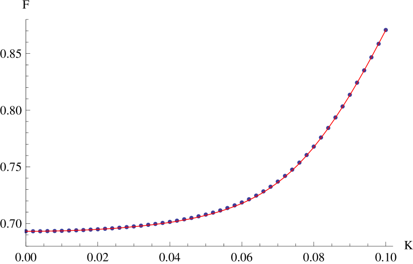
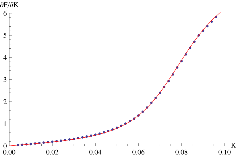
Figure 5: Left: free energy (red curve) compared to the formula (139) (points) for $K_{16,16}$. Right: internal energy (red curve) compared to the derivative of the points produced by (139) (points) for $K_{16,16}$.

XI Lattices

The plots in figure 4 are very representative for several graphs of interest. We intend to focus on the graphs that traditionally are studied in statistical physics; lattice graphs. We will take a look at the simple lattices in 1, 2, 3, 4 and 5 dimensions. Just to be clear, a 1D-lattice is a cycle $C_{n}$ on $n$ vertices and it is $2$-regular, i.e. $2$ neighbours for each vertex. The 2-dimensional $L\times L$-lattice is the cartesian product of two cycles on $L$ vertices. The product thus has $n=L^{2}$ vertices and it is $4$-regular. The $d$-dimensional $L\times L\times\cdots\times L$-lattice is a product of $d$ cycles on $L$ vertices, thus having a total of $n=L^{d}$ vertices. It is obviously $2\,d$-regular. Assuming finite-size scaling to hold then for a $d$-dimensional lattice we have

$$\sigma_{1}=n\,\bar{\mu}/2\propto n\,L^{-\beta/\nu}=n\,\left(n^{1/d}\right)^{-\beta/\nu}=n^{1-\beta/d\,\nu}$$ (141)

and correspondingly for the second moment

$$\sigma_{2}=n\,\chi/4\propto n\,L^{\gamma/\nu}=n\,\left(n^{1/d}\right)^{\gamma/\nu}=n^{1+\gamma/d\,\nu}$$ (142)

Note also that for an $r$-regular triangle-free graphs we have $\mathbb{P}\left(M=n\right)=\mathbb{P}\left(M=n-2\right)$ when $K=\frac{\log n}{2\,r}$.

XI.1 1D-lattices

For 1D-lattices we can compute the coefficients $a(E,M)$ exactly. It is an exercise to show that the number of states with $k$ negative spins and $\ell$ negative spin products (over the edges) is

$$a(E,M)=\binom{k}{k-\ell/2}\,\binom{n-k-1}{n-k-\ell/2}+\binom{k-1}{k-\ell/2}\,\binom{n-k}{n-k-\ell/2}$$ (143)

where $M=n-2\,k$ and $E=n-2\,\ell$. The distribution of magnetisations do not behave in a way representative for lattices of higher dimension. However, for extremely low temperatures the probabilities $\mathbb{P}\left(M=-n\right)=\mathbb{P}\left(M=n\right)$ will dominate the other probabilities. The two outermost probabilities, $\mathbb{P}\left(M=n\right)$ and $\mathbb{P}\left(M=n-2\right)$, are equal when $K=\frac{\log n}{4}$. For the 1D-lattice the distribution is here sharply unimodal, while for higher dimensions the distribution is bimodal and has its peaks at the extreme magnetisations. For $K$ larger than $(\log n)/4$ the distribution actually has three peaks, i.e. a local maximum at $M=0$. For 1D-lattices the $p,q$-approximation of the distribution thus breaks down beyond this $K$ since it can not model a local maximum in the middle as well as peaks at the ends; they are at most bimodal. For $K$ less than this point the $p,q$-distribution is a very good approximation. Figure 6 demonstrates this clearly; for the flattest distribution (low temperature) the fitted $p,q$-distribution starts to deviate from the actual distribution. In figure 7 we plot $y=n\,(p-1)$ and $z=n\,(q-1)$ versus $K$ for a range of different $n$. Clearly there is some limit curve here, though we have not established what the limit function is.

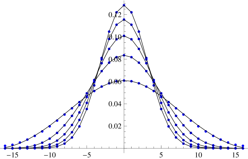
Figure 6: Magnetisation distributions for $C_{32}$ (points) and fitted $\mathbb{P}_{p,q}\left(n,\,k\right)$ (lines) vs $k-n/2$ for several temperatures.

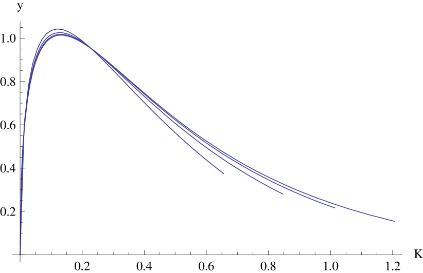
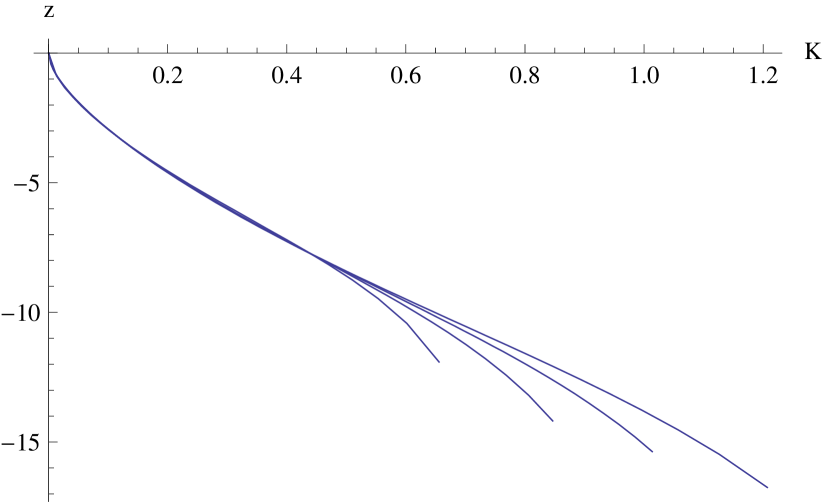
Figure 7: Left: $y=n\,(p-1)$ versus $K$ for $C_{n}$. Right: $z=n\,(q-1)$ versus $K$ for $C_{n}$. Both plots are for $n=16,32,64,128$ (larger cycles stretch farther to the right).

In figure 8 we see $y=n\,(p-1)$ versus $z=n\,(q-1)$ for different $n$. The right plot of figure 8 shows the value at $K$ that gives the maximum value of $y$. The fitted straight line gives the limit $0.1333$, very close to $2/15$.

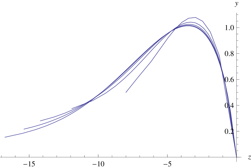
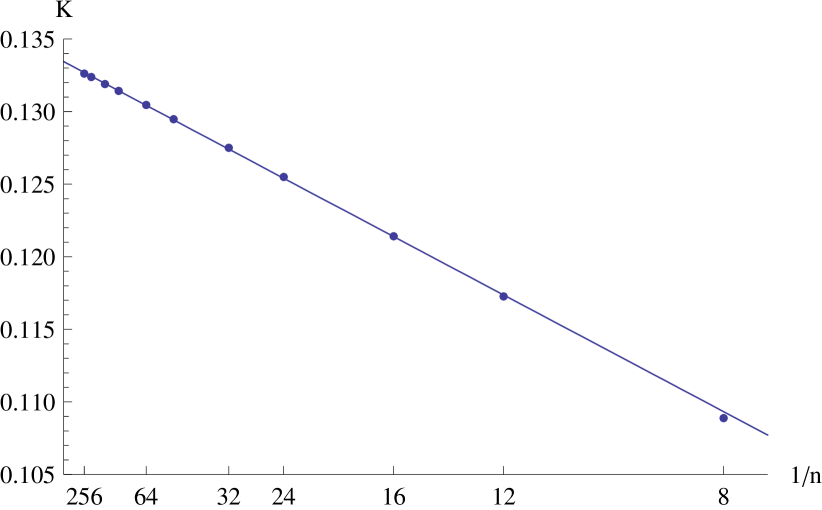
Figure 8: Left: $y=n\,(p-1)$ versus $z=n\,(q-1)$ for $C_{n}$, with $n=8,16,32,64,128$ with larger $n$ extending farther to the left. Right: $K$ giving the maximum $y$ vs $1/n$ for $C_{n}$, $n=8$, 12, 16, 24, 32, 48, 64, 96, 128, 192, 256.

What about the values of $y$ and $z$? Indeed they converge beautifully as figure 9 indicates. The limit for $y$ is about $1.010$ and $z$ approaches a value of $-3.537$.

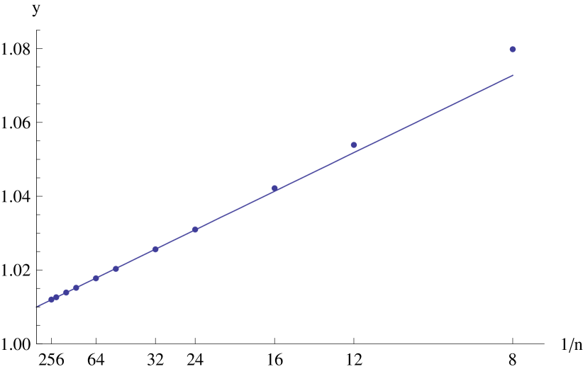
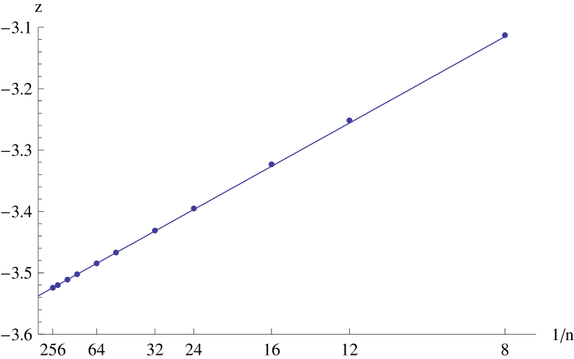
Figure 9: Left: Maximum value of $y=n\,(p-1)$ versus $1/n$ for $C_{n}$. Right: value of $z\,(q-1)$ versus $1/n$ for $C_{n}$ when $y$ is at its maximum. In both cases $n=8$, 12, 16, 24, 32, 48, 64, 96, 128, 192, 256.

Though we can not exactly solve what $y$ and $z$ should be at $K=2/15$ we can at least see how $y$ and $z$ relate at this point. For an infinite 1-dimensional lattice we have that $\chi=e^{2\,K}$, see e.g. Baxter (1982). The second moment then should behave as

$$\sigma_{2}\sim\frac{n\,\chi}{4}=\frac{n\,e^{2\,K}}{4}$$ (144)

Let $\ell=k-n/2$ and $\sigma=\sqrt{\sigma_{2}}$. For high temperatures we expect $\ell/\sigma$ to be normally distributed and thus

$$\mathbb{P}\left(\ell\right)\sim\frac{\exp\left(-(\ell/\sigma)^{2}/2\right)}{\sigma\,\sqrt{2\,\pi}}$$ (145)

The probability ratio is then

$$R\left(n,\,n/2,\,\ell\right)=\frac{\mathbb{P}\left(\ell\right)}{\mathbb{P}\left(0\right)}=\exp\left(-\ell^{2}/2\,\sigma^{2}\right)$$ (146)

and for $\ell=1$ this simplifies to

$$R\left(n,\,n/2,\,1\right)=\exp\left(-1/2\,\sigma^{2}\right)=\exp\left(-2\,e^{-2\,K}/n\right)\sim 1-\frac{2\,e^{-2\,K}}{n}$$ (147)

Compare this with (66). We thus have $a=-2\,e^{-2\,K}$. Now $y$ and $z$ are related as $y=2\,w-a$ where $w$ is defined by (68). If we set $K=2/15$ then $a=-1.531857$, and choosing $z=-3.537$ indeed gives us $y=1.01002$. To actually solve $z$ as a function of $K$ seems harder though. However, numerical experimentation suggests that $y$ and $z$ for small $K$ behave as

$$y(K)\approx c_{1}\,\sqrt{K}+c_{2}\,K$$ (148)

$$z(K)\approx-c_{1}\,\sqrt{K}+c_{2}\,K$$ (149)

where $c_{1}\approx 6.164$ and $c_{2}\approx-10.33$.

Strangely, when the $p,q$-distribution fit the magnetisation distribution so well one might think that the free energy would be well approximated by (139). This is not so. The $p,q$-approximation differs clearly from the asymptotic free energy, given by $\log\left(2\,\cosh K\right)$.

XI.2 2D-lattices

For the 2-dimensional lattices we can rely on exact data only for up to $L=16$ and they were computed according to the method in Häggkvist and Lundow (2002). We have sampled data for $L=32,64,128,256,512$, collected with the methods described in Häggkvist et al. (2004) and Lundow and Markström (2009a). These methods gave us the energy distribution and then it is just a matter of combining this with the distribution of magnetisations for each given energy as described in Häggkvist et al. (2007). Figure 10 shows an example of some distributions for the $128\times 128$-lattice together with their fitted $p,q$-binomial distributions. The fit is fairly good, but hardly excellent near $K^{*}$. However, as the figure shows, at $K=0.4388$ (i.e. for $L=128$) the fit is practically spot on. For the lattices we have studied there is always one such temperature where the $p,q$-distribution fit particularly well. This point is located between $K^{*}$ and $K_{c}$ and is very close to, but not exactly equal to, the point where the susceptibility is at its maximum.

Of course, for high temperatures (small $K$) and low temperatures (high $K$) the fit is typically very good but in the high-temperature region the measured $y$ and $z$ are unfortunately extremely sensitive to noise. As we get closer to the critical region where the distribution becomes bimodal this problem goes away, even though the sampled distributions are more noisy there. Regarding the free energy it is well-fitted by (139) for low temperatures $K>K^{*}$ though less well for high temperatures $K<K^{*}$.

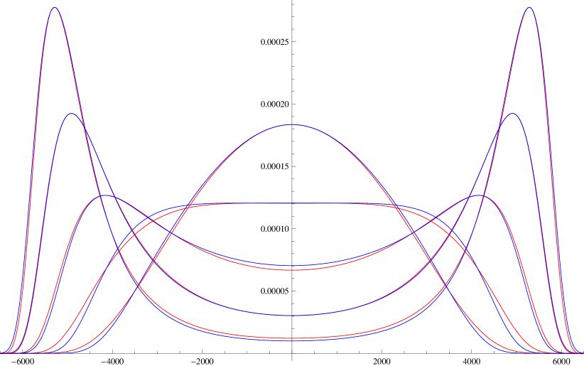
Figure 10: Magnetisation distributions for the $128\times 128$-lattice (red) together with fitted $p,q$-binomial distributions $\mathbb{P}_{p,q}\left(n,\,k\right)$ (blue) vs $k-n/2$ at $K=0.432$, $K^{*}=0.43467$, $K=0.437$, $K=0.4388$ and $K_{c}=0.44068$ (downwards at $y$-axis).

Recall from section IX how the exponents of the moment growth rates could be computed if we allow $z$ to depend on $n$. For the 2D-lattices it is known that $\beta=1/8$, $\gamma=7/4$ and $\nu=1$, see Onsager (1944), Yang (1952) and Abraham (1978). Thus the first moment $\sigma_{1}$ should scale as $n^{15/16}$ and the second moment $\sigma_{2}$ as $n^{15/8}$. From equation (108) and (109) this would be achieved by choosing $\lambda_{1}=-3/2$, $\lambda_{2}=-6$ and $\lambda_{3}=0$. The left plot of Figure 11 shows $z$ versus $\log n$ at $K^{*}$ together with the curve $3-1.5\,\log n-6\log\log n$. The constant $\lambda_{0}$ is chosen only to make the curve look plausibly near the points. The point for $L=512$ deviate slightly but we suspect that noise in the sampled data explains this. With $\lambda_{0}=3$ the coefficient of $n^{15/8}$ obtained from (109) would be $0.301$ though the measured $\sigma_{2}$ divided by $n^{15/8}$ are closer $0.08$. To get this we have to choose $\lambda_{0}\approx 8.3$. In that case the convergence is extremely slow. Note also that the fitted $p,q$-distribution is far from perfect which would contribute some amount of error as well.

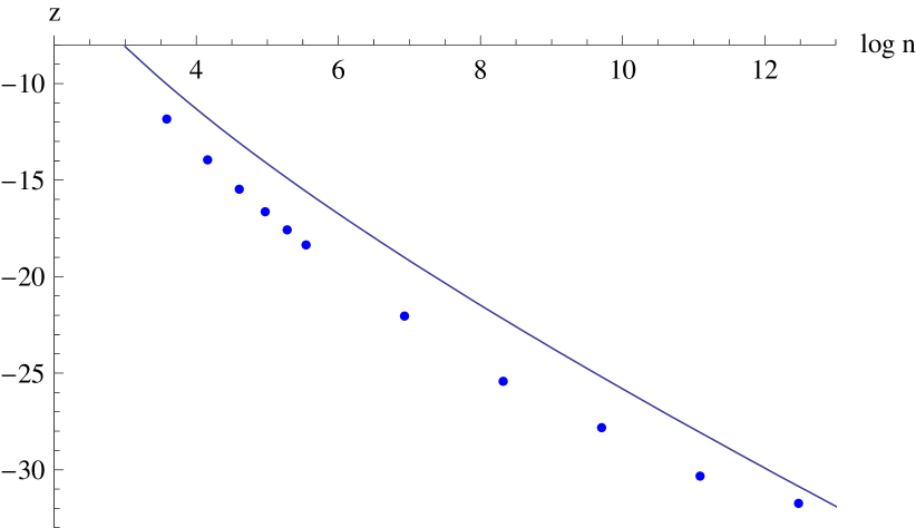
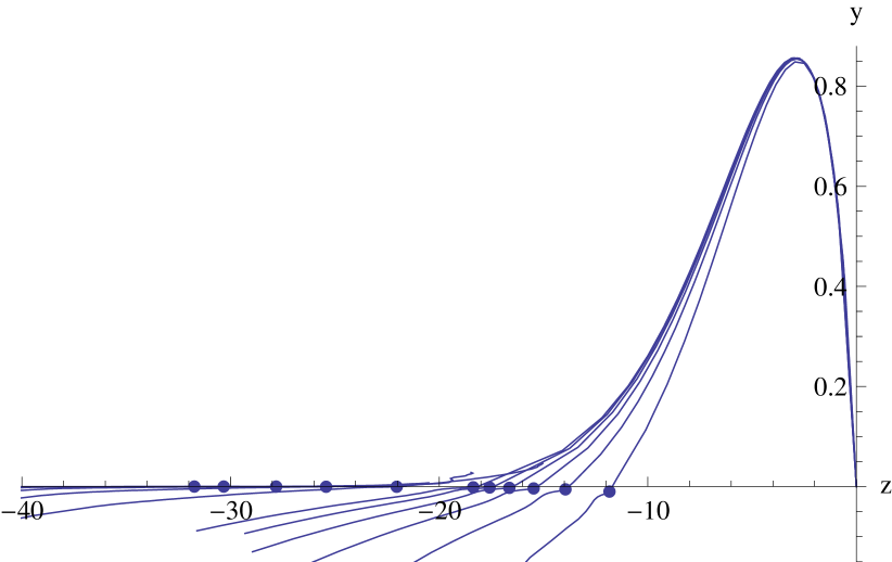
Figure 11: Left: $z=n\,(q-1)$ vs $\log n$ at $K^{*}$ for the $L\times L$-lattice, $L=6$,  8, 10, 12, 14, 16, 32, 64, 128, 256, 512. The curve is $3-1.5\,\log n-6\,\log\log n$. Right: $y=n\,(p-1)$ vs $z=n\,(q-1)$ for the $L\times L$-lattice, $L=6$, 8, 10, 12, 14, 16, 32, 64, 128, 256, 512 (512 barely visible near the $z$-axis). The points represent $K^{*}$.

The right plot of figure 11 shows $y$ vs $z$ for a range of temperatures. The points representing $K^{*}$ may appear to lie on the $z$-axis but they are are slightly below it. In the 1D-case we suspected that there is a limit curve for the high-temperature region, but we suspect that the exact data that produced this part of the plot rely on far too small lattices to give any conclusive evidence. Also, the $p,q$-find algorithm is rather sensitive to noise in this region to be useful for sampled data. However, as we said before, this problem goes away once $K\geq K^{*}$. Figure 12 shows $y$ and $z$ versus $K$ for all the lattices though for the sampled data we only show low-temperature data. The red line is located at $K_{c}=\operatorname{atanh}{\left(\sqrt{2}-1\right)}\approx 0.44068$.

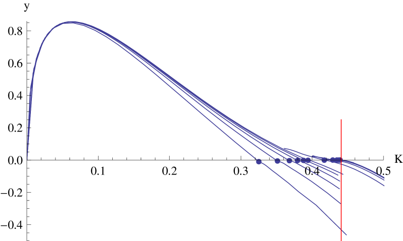
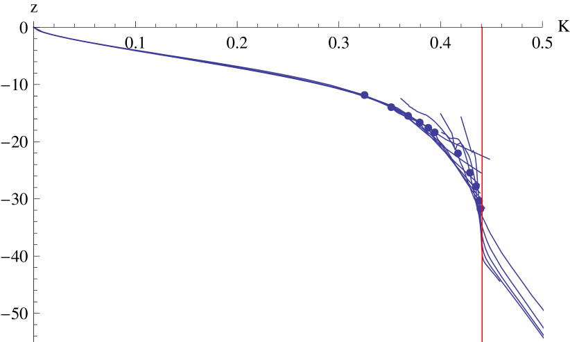
Figure 12: $y=n\,(p-1)$ vs $K$ (left) and $z=n\,(q-1)$ vs $K$ (right) for the $L\times L$-lattice, $L=6$, 8, 10, 12, 14, 16, 32, 64, 128, 256, 512. The points represent $K^{*}$ and the red line is at $K_{c}$. The larger lattices have their points farther to the right in the plots.

XI.3 3D-lattices

For these lattices we only have exact data for $L=4$ and sampled data for $L=6,8,12,16,32,64$. The situation is actually somewhat better for 3D-lattices. Figure 13 shows some distributions in the vicinity of $K^{*}$ for $L=32$ together with the fitted $p,q$-distributions. For $K\geq K^{*}$, just when the distributions become bimodal, the fit is certainly less than perfect, but near $K^{*}$ the $p,q$-approximation is actually rather good.

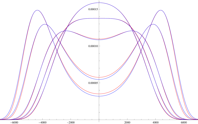
Figure 13: Magnetisation distributions for the $32\times 32\times 32$-lattice (red) and the fitted $\mathbb{P}_{p,q}\left(n,\,k\right)$ (blue) vs $k-n/2$ for $K=0.2204$, $K^{*}=0.22066$, $K=0.2210$, $K_{c}=0.2216546$ and $0.2220$ (downwards at the y-axis).

In the left plot of figure 14 we show $z$ versus $\log n$ at $K^{*}$. The fitted line through the points corresponds to $z=-5.3-\log n$ and is not too bad an approximation. However, in Häggkvist et al. (2007) it was estimated that the growth rate exponent at $K_{c}$ of the susceptibility is $\gamma/\nu=1.978\pm 0.009$ (assuming $\gamma=\gamma^{\prime}$ and $\nu=\nu^{\prime}$). For the magnetisation it was estimated $\beta/\nu=0.5147\pm 0.0007$. Translated into exponents of $n$ this means $1.657\leq 1+\gamma/3\nu\leq 1.663$ and $0.8282\leq 1-\beta/3\nu\leq 0.8287$. If we choose $\lambda_{1}=-5/8$ in (108) and (109) the first moment exponent would be $53/64=0.828125$ and $53/32=1.65625$ for the second moment, slightly below the lower bound of the estimate intervals. Choosing $\lambda_{1}=-2/3$ would give exponents $5/6=0.8333\ldots$ and $5/3=1.666\ldots$ respectively, slightly above the upper bound of the intervals. Let us suggest, as an example, that $\lambda_{0}=6.8$, $\lambda_{1}=-2/3$, $\lambda_{2}=-6$ and $\lambda_{3}=0$ in the expression (109). In figure 14 the curve use these parameters for $z$ at $K^{*}$, i.e. $z=6.8-(2/3)\,\log n-6\,\log\log n$. Will the points eventually converge to the curve? It would take considerably larger lattices to shed any light on this. We also have the problem what $\lambda_{0}$ should be. Using $\lambda_{0}=6.8$ means that the coefficient in (109) is about $0.393$. Comparing the measured $\sigma_{2}$ with $n^{5/3}$ gives a factor of roughly $0.16$ though the data are certainly far from conclusive. Since the distribution fit is not perfect a different constant is perhaps to be expected. Also, slow convergence is to be expected here.

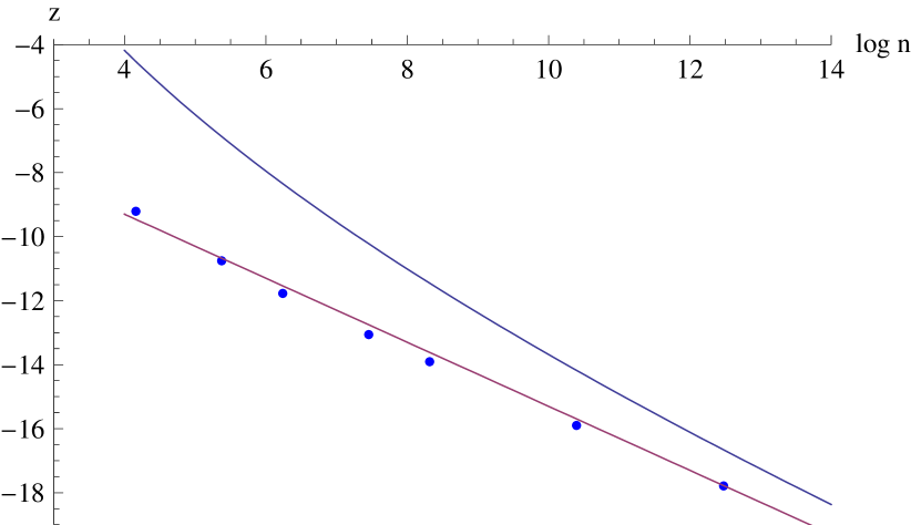
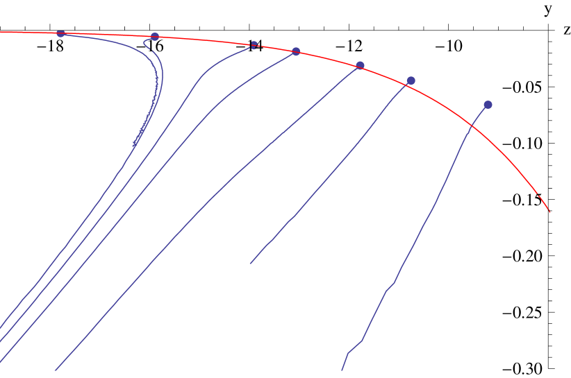
Figure 14: Left: $z=n\,(q-1)$ vs $\log n$ at $K^{*}$ for the $L\times L\times L$-lattice, $L=4,6,8,12,16,32,64$. The line though the points is $-5.3-\log n$ and the curve is $6.8-(2/3)\,\log n-6\,\log\log n$. Right: $y=n\,(p-1)$ vs $z$ for the $L\times L\times L$-lattice, $L=4,6,8,12,16,32,64$ (leftwards) for $K>K^{*}$. Higher values of $K$ when we move downwards left. The red curve is $y=2\,w$ with $w$ defined by (59).

The right plot of figure 14 shows $y$ versus $z$ for $K>K^{*}$. Note the peculiar backwards movement of $z$ getting more and more pronounced for larger $L$. The curves for $16$, $32$ and $64$ show signs of approaching some limit curve. We don’t have data for very low temperatures for the smaller lattices though, except for $L=4$. The plots in figure 15 shows $y$ and $z$ versus $K$ for $K>K^{*}$. The red lines show location of $K_{c}\approx 0.2216546$, found in Häggkvist et al. (2007), but see also Rosengren (1986) for a theoretical estimate of $K_{c}$.

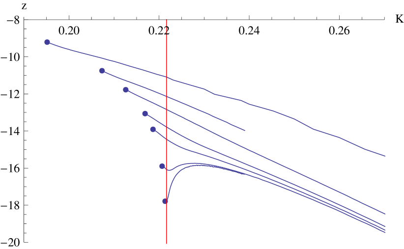
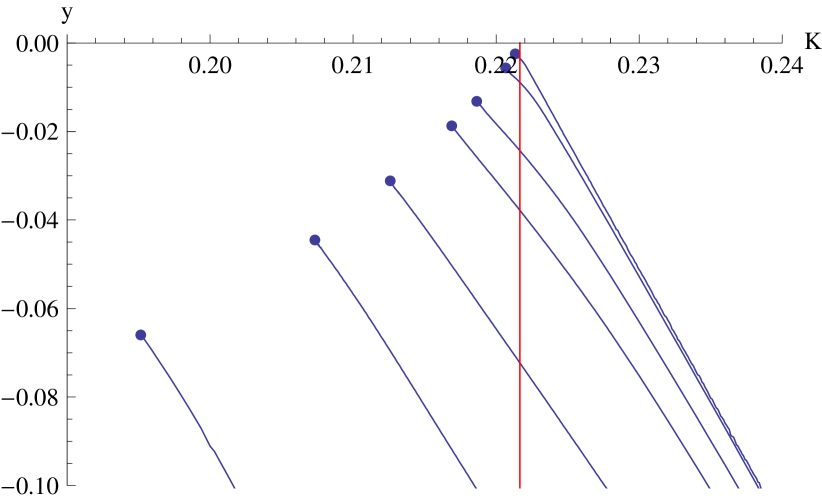
Figure 15: Left: $z=n\,(q-1)$ vs $K$ with $K>K^{*}$ for the $L\times L\times L$-lattice, $L=4,6,8,12,16,32,64$ (downwards). Right: $y=n\,(p-1)$ vs $K$ with $K>K^{*}$ for the $L\times L\times L$-lattice, $L=4,6,8,12,16,32,64$ (upwards). In both plots the red line indicates location of $K_{c}$ and the points are the locations of $K^{*}$.

XI.4 4D-lattices

In the case of 4-dimensional lattices we have sampled data of magnetisation distributions for $L=4,6,8,10,12,16$. Figure 16 shows some of these magnetisation distributions for $L=12$ near $K^{*}$ together with fitted $p,q$-binomial distributions. The fit is quite good, considerably better than for 2D and 3D, in the whole range of selected temperatures. Though it is hard to distinguish the fitted curves from the magnetisation curves, there is a small deviation near the middle.

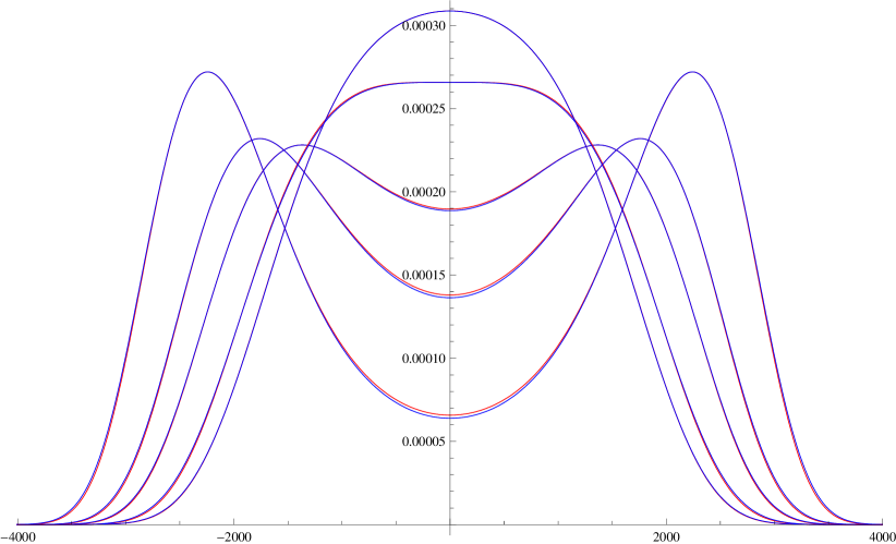
Figure 16: Magnetisation distributions for the $12\times 12\times 12\times 12$-lattice (red) and the fitted $\mathbb{P}_{p,q}\left(n,\,k\right)$ (blue) vs $k-n/2$ for $K=0.1490$, $K^{*}=0.149255$, $K_{c}=0.149695$, $K=0.1500$ and $K=0.1505$ (downwards at the y-axis).

How should $z$ at $K^{*}$ depend on $n$? Actually, taking the data at face-value they are rather well-fitted to the simple formula $z=-6.5-0.45\,\log n$. However, for the 4D-lattice we have $\gamma=\gamma^{\prime}=1$, $\beta=1/2$ and $\nu=\nu^{\prime}=1/2$. This gives that $1+\gamma/d\,\nu=3/2$ and $1-\beta/d\,\nu=3/4$. Moreover, according to Lai and Mon (1990) there should be a correction to this. They calculated, using renormalization group techniques, that the susceptibility should scale as $L^{2}\,\sqrt{\log L}$ near $K_{c}$. This means that $\sigma_{2}$ should scale as $n^{3/2}\,\sqrt{\log n}$. From (112) we see that we have to choose $\lambda_{2}=-2$, with $\lambda_{1}=0$ and $\lambda_{3}=-6$, to obtain this. In the left plot of figure 17 we have set $z=-1.2-2\,\log\log n-6\log\log\log n$ and plotted it versus $\log\log n$. The curve would then behave as a limit curve rather than as a fitted curve. The choice of coefficient $\lambda_{0}=-1.2$ is only supported by the human eye as a guide rather than any theory and herein lies a problem. With this choice the coefficient of (112) is about $0.558$. However, dividing the measured $\sigma_{2}$ at the different $K^{*}$ with $n^{3/2}\,\sqrt{\log n}$ gives values close to $0.15$. This discrepancy could be due to several sources; e.g. the expression in (112) could be incorrect or our data could be suffering from very slow convergence.

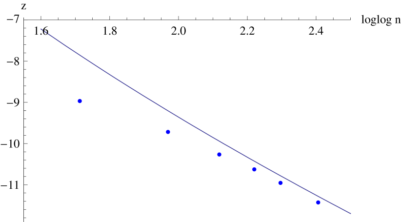
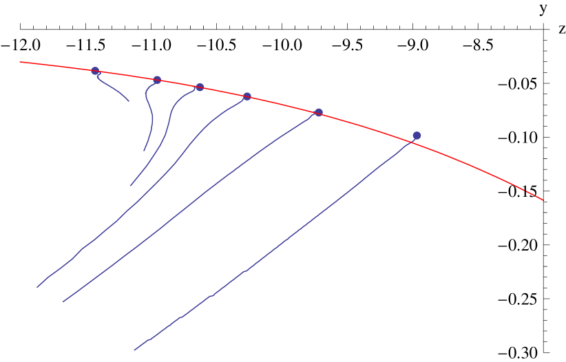
Figure 17: Left: $z=n\,(q-1)$ vs $\log\log n$ at $K^{*}$ for the $L\times L\times L\times L$-lattice, $L=4,6,8,10,12,16$. The curve is $-1.2-2\,\log\log n-6\,\log\log\log n$. Right: $y=n\,(p-1)$ vs $z=n\,(q-1)$ for the $L\times L\times L\times L$-lattice, $L=4,6,8,10,12,16$ (leftwards). Higher temperatures (low $K$) begin at the upper right part of the plot and with lower temperatures we move down to the left. The red curve is $y=2\,w$ with $w$ defined by (59).

In the right plot of figure 17 we show $y$ versus $z$ for $K>K^{*}$ together with the curve $y=2\,w$ with $w$ defined by (59). In figure 18 we show $y$ and $z$ versus $K$ for $K>K^{*}$. The red line is located at $K_{c}\approx 0.1496497$, estimated in Lundow and Markström (2009b).

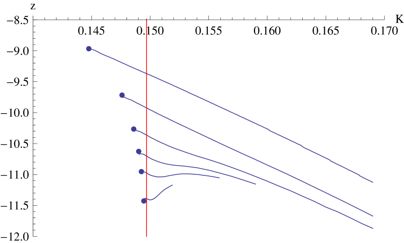
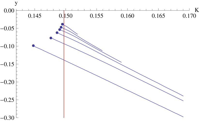
Figure 18: Left: $z=n\,(q-1)$ vs $K$ with $K>K^{*}$ for the $L\times L\times L\times L$-lattice, $L=4,6,8,10,12,16$ (downwards). Right: $y=n\,(p-1)$ vs $K$ with $K>K^{*}$ for the $L\times L\times L\times L$-lattice, $L=4,6,8,10,12,16$ (upwards). In both plots the red line indicates location of $K_{c}$ and the points are the locations of $K^{*}$.

XI.5 5D-lattices

For the 5-dimensional lattices we have sampled data of magnetisation distributions only for $L=4,6,8,10,12$. The distributions in figure 19 are extremely well fitted by $p,q$-binomial distributions; it is almost impossible to tell them apart with the naked eye.

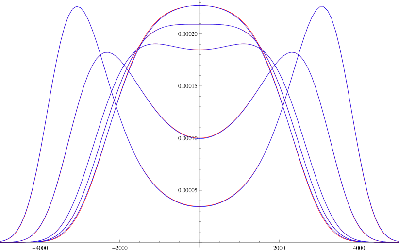
Figure 19: Magnetisation distributions for $8\times 8\times 8\times 8\times 8$-lattice (red) and the fitted $\mathbb{P}_{p,q}\left(n,\,k\right)$ (blue) vs $k-n/2$ for $K=0.1137$, $K^{*}=0.113786$, $K_{c}=0.113914$, $0.1143$ and $0.1147$.

In five dimensions the susceptibility near $K_{c}$ scales as $L^{5/2}$, see Cardy (1996). Thus $\sigma_{2}$ should scale as $n^{3/2}$ which is exactly what we receive when keeping $z$ fixed. So, for $z$ constant we obtain $\sigma_{1}\propto n^{3/4}$ and $\sigma_{2}\propto n^{3/2}$.

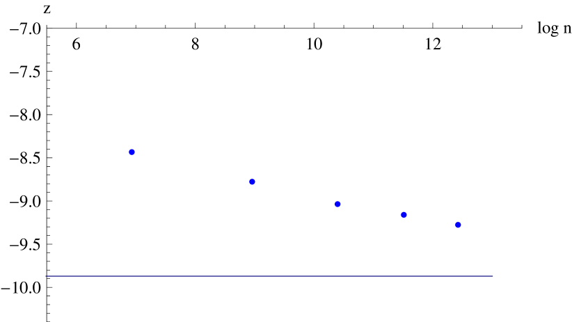
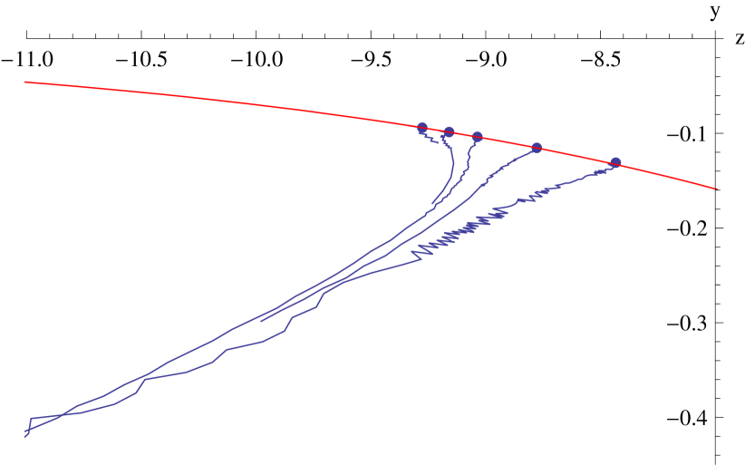
Figure 20: Left: $z=n\,(q-1)$ vs $\log n$ at $K^{*}$ for the $L\times L\times L\times L\times L$-lattice, $L=4,6,8,10,12$. The straight line is constant at $z=-9.87$. Right: $y=n\,(p-1)$ vs $z=n\,(q-1)$ for the $L\times L\times L\times L\times L$-lattice, $L=4,6,8,10,12$ (leftwards). Higher temperatures (low $K$) begin at the upper right part of the plot and with lower temperatures we move down to the left. The red curve is $y=2\,w$ with $w$ defined by (59).

The left plot of figure 20 shows $z$ at $K^{*}$ for $L=4,6,8,10,12$. If $z$ approaches a constant then what is the limit value? Extracting the limit $z$ from this plot is futile of course. The right plot of figure 20 shows $y$ vs $z$ for the different lattices together with the points $K^{*}$ and the curve $y=2\,w$.

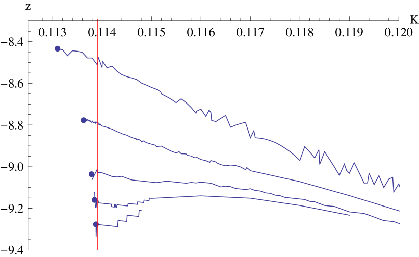
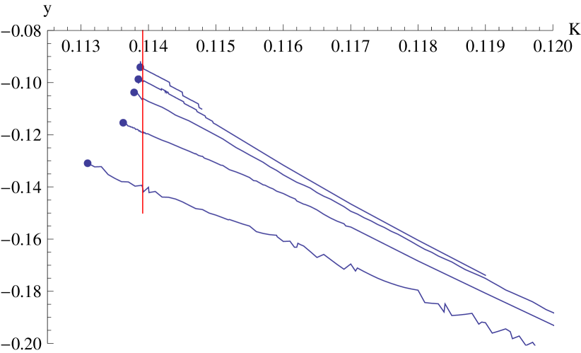
Figure 21: Left: $z=n\,(q-1)$ vs $K$ with $K>K^{*}$ for the $L\times L\times L\times L\times L$-lattice, $L=4,6,8,10,12$ (downwards). Right: $y=n\,(p-1)$ vs $K$ with $K>K^{*}$ for the $L\times L\times L\times L\times L$-lattice, $L=4,6,8,10,12$ (upwards). In both plots the red line indicates location of $K_{c}$ and the points are the locations of $K^{*}$.

In figure 21 we show $y$ and $z$ versus $K$ for $K\geq K^{*}$ with an estimated $K_{c}$ marked as a red line. Despite the noise in the plots it seems plausible that $z$ stays essentially constant very close to $K^{*}$ (and $K_{c}$) and that only $y$ moves. Let us assume this and see where this leads us. We employ the moment expressions in section VIII in terms of the parameter $a$ to model the behaviour near $K^{*}$. A normalised first cumulant of the absolute magnetisation $\left\langle\left\lvert M\right\rvert\right\rangle/2\,n^{3/4}=\sigma_{1}/n^{3/4}$ should approach $\varrho_{1}/\varrho_{0}$ when plotted as a function of $a$ for a fixed $z$. Analogously, the second cumulant (normalised) should behave as

$$\frac{\sigma_{2}-\sigma_{1}^{2}}{n^{3/2}}\to\frac{\varrho_{2}}{\varrho_{0}}$$ (150)

where the $\varrho_{m}$ were defined in section VIII. Note that for a fixed $z$ the $\varrho_{m}$ now depend only on $a$. The third and fourth cumulants of the absolute magnetisation, divided by respectively $8\,n^{9/4}$ and $16\,n^{3}$, quite analogously approach their corresponding limits

$$\frac{\varrho_{3}}{\varrho_{0}}-3\,\frac{\varrho_{1}\,\sigma_{2}}{\varrho_{0}^{2}}+2\,\frac{\varrho_{1}^{3}}{\varrho_{0}^{3}}$$ (151)

and

$$\frac{\varrho_{4}}{\varrho_{0}}-4\,\frac{\varrho_{1}\,\sigma_{3}}{\varrho_{0}^{2}}-3\,\frac{\sigma_{2}^{2}}{\varrho_{0}^{2}}+12\,\frac{\varrho_{1}^{2}\,\varrho_{2}}{\varrho_{0}^{3}}-6\,\frac{\varrho_{1}^{4}}{\varrho_{0}^{4}}$$ (152)

Through a simple scaling analysis based on our sampled data we have found that the normalised third cumulant has a limit maximum of about $0.0205$ and a minimum of $-0.0500$. The fourth normalised cumulant has a limit maximum of $0.0229$ and a minimum of $-0.0278$, based upon our sampled data. Choosing $z=-9.87$ puts the maximums and minimums of the limit curves at appropriate values. Now we identify the coupling $K$ where the minimum of the fourth cumulant occurs with the point $a$ where the minimum of the corresponding limit curve occurs and likewise for the maximum, thus providing us with a rescaling translating $K$ into $a$. In figure 22 and 23 the first four cumulants are shown together with their estimated limit curves for $z=-9.87$. Indeed the red curve may provide us with a limit.

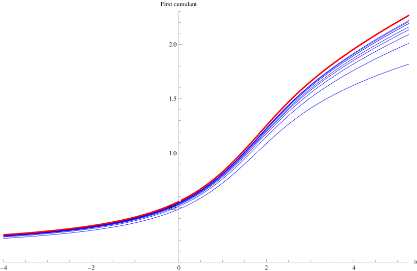
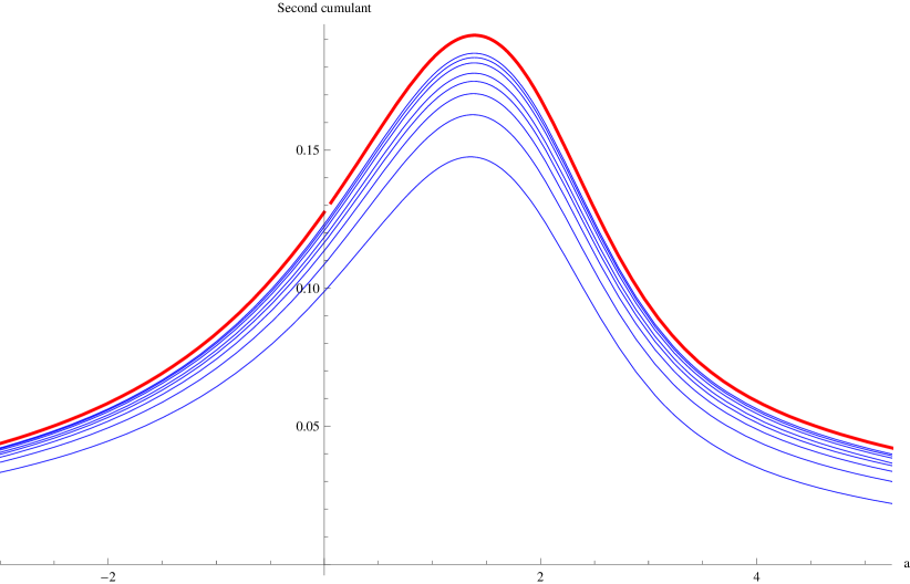
Figure 22: Normalised first (left) and second (right) cumulants for the $L\times L\times L\times L\times L$-lattice, $L=4,6,8,10,12,16,20,24$ (blue) versus $a$ for $z=-9.87$ together with the limit curve (red).

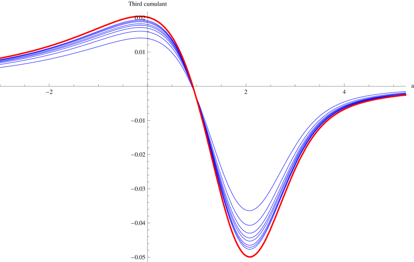
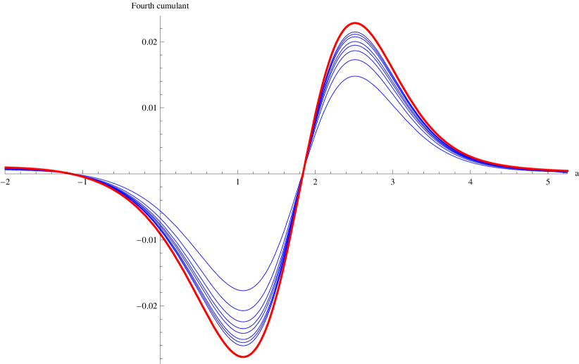
Figure 23: Normalised third (left) and fourth (right) cumulants for the $L\times L\times L\times L\times L$-lattice, $L=4,6,8,10,12,16,20,24$ (blue) versus $a$ for $z=-9.87$ together with the limit curve (red).

Given a lattice size $L$ we denote by $K_{\min}(L)$ the location of the minimum fourth cumulant and by $K_{\max}(L)$ the location of the maximum. Analogously for the limit curve, given a $z$ we denote by $a_{\min}(z)$ and $a_{\max}(z)$ the location of the minimum and maximum fourth cumulant. For $z=-9.87$ we have $a_{\min}\approx 1.06965$ and $a_{\max}\approx 2.51275$. A simple scaling projection gives that roughly $K_{\max}(L)\approx K_{c}+0.22/L^{5/2}$ and $K_{\max}(L)-K_{\min}(L)\approx 0.093/L^{5/2}$. Also $K_{c}\approx 0.113915$, see Luijten et al. (1999). Thus, in principle at least, the rescaling between $a$ and $K$ is

$$K(a)\sim\frac{K_{\max}(L)-K_{\min}(L)}{a_{\max}(z)-a_{\min}(z)}\,\left(a-a_{\max}(z)\right)+K_{\max}(L)$$ (153)

However, this kind of expression is somewhat too simplistic to get figure 23. It would take higher-order corrections to scaling to produce it but this would probably take a more involved numerical study of the 5D-model. Other investigations of the 5D-lattice includes e.g. Brezin and Zinn-Justin (1985), Mon (1996) and Luijten et al. (1999).

XII Conclusions

The magnetisation distribution for the complete graph is exactly described by the $p,q$-binomial distribution, corresponding to the special (or limit) case of $p=q$. For balanced complete bipartite graphs this is most likely also true in some limit sense, yet to be made precise. Actually, it appears that for most graphs, at least those which are more or less regular, the magnetisations are well-fitted by a $p,q$-binomial distribution for some choice of $p$ and $q$. The exact extent to which the $p,q$-binomial approximation is good we do not yet know (e.g. convergence in moment) nor the exact class of graphs that would satisfy this. We have investigated the matter more closely for lattices of dimension one through five. In general they are always well-fitted by $p,q$-binomial distributions for high- and low-temperatures but the problems arise near $K_{c}$, or rather $K^{*}$ where the distribution changes from unimodal to bimodal.

For the 1-dimensional lattices (having no such bounded $K^{*}$) the situation is basically always that of high temperatures. It seems possible to give expressions for $p$ and $q$ in terms of $K$ in this case though we have not done so. For 2-dimensional lattices the distributions near $K^{*}$ are least well-fitted by the $p,q$-binomials but slightly better fitted in the 3-dimensional case. We made theory-based predictions of how $z$ should scale with $n$ near $K^{*}$. Unfortunately, scaling is probably very slow, involving logarithms and double logarithms, making it near impossible to test the prediction. For 4-dimensional lattices the distributions are clearly much better fitted by $p,q$-binomials, though some discrepancy still remains just above $K^{*}$. For 5-dimensional lattices even this small discrepancy is gone, leaving us perfectly fitted (that is, to the human eye) $p,q$-binomial distributions. In this case the values of $z$ at $K^{*}$ should approach a limit value. We estimated this limit and, using this limit value, compared the first four normalised cumulants for finite lattices with the (possible) limit curves.

We described and used a rather simple method to determine $p$ and $q$ given a distribution. Possibly this method is not optimal since it simply forces the distribution to be correct at a single point rather than providing a good overall-fit. It is also sensitive to noise when the distributions are unimodal, thus making it difficult to determine $p$ and $q$. On the other hand it works extremely well for bimodal distributions where the noise sensitivity problem vanishes.

The $p,q$-binomial coefficients are just a tweaked form of $q$-binomials, i.e. they are multiplied by a power of $p$. It is possible that a different choice of factor would produce better results in the case of 2- and 3-dimensional lattices.

We believe that what is said here for the Ising model also goes for other models, i.e. the magnetisation distribution for quantum spin models or for spin-glass models can be modeled by $p,q$-binomial distributions.