Light cone QCD sum rules for the $g_{\Xi_{Q}\Xi_{Q}\pi}$ coupling constant

Abstract

For the heavy baryons $\Xi_{c}$ and $\Xi_{b}$ the coupling constants $g_{\Xi_{c}\Xi_{c}\pi}$ and $g_{\Xi_{b}\Xi_{b}\pi}$ are calculated in the framework of light cone QCD sum rules. The most general form of the interpolating field of $\Xi_{Q}$ is used in the calculation.

I Introduction

Experimental progresses over the last few years provided exciting results in the heavy baryon sector. There have been plenty of heavy baryon observations yielding a large amount of experimental data on charm and bottom baryons. Observation of Belle, BABAR, DELPHI, CLEO, CDF, DO etc Mizuk2005 ; Mizuk2007 ; Aubert2007 ; Feindt2007 ; Edwards1995 ; Artuso2001 ; I.V.Gorelov2007 ; Aaltonen2007 ; Abazov2007 have motivated the theoretical interests on heavy baryons containing c and b quarks. The mass spectroscopy of these baryons have been studied using various theoretical models Capstick ; Roncaglia ; Jenkins ; Mathur ; Ebert ; Karliner1 ; Karliner2 ; Rosner ; Karliner3 as well as QCD sum rules method Shifman ; Bagan ; Navarra ; Shuryak ; Grozin ; Dai ; Wang1 ; Zhu1 ; Huang ; Wang2 ; Wang3 ; Duraes ; Liu . Their masses calculated via QCD sum rules in heavy quark limit Shuryak and in the heavy quark effective theoryGrozin ; Dai ; Wang1 .

Beside the mass spectrum there have been theoretical studies on the magnetic moments of these baryons utilizing naive quark model Choudhury ; Lic , quark model Glozman ; Julia , bound state approach Schollamd , relativistic three-quark model Faessler , hyper central model Patel , Chiral perturbation model Savage , soliton model DOR , skyrmion model Oh , nonrelativistic constituent quark model An , QCD sum rules in external magnetic fiels Zhu2 , and light cone QCD sum rules (LCQSR) method Aliev1 ; Aliev2 .

In the present work we make use of the (LCQSR) to calculate the coupling constant $g_{\Xi_{Q}\Xi_{Q}\pi}$. A similar work has been done in Azizi for the coupling constant $g_{\Sigma_{Q}\Lambda_{Q}\pi}$. This paper is organized as follows. In section 2, we introduce the interpolating field for $\Xi_{Q}$ and give the details of (LCQSR) calculations for the coupling constant. In section 3 the numerical analysis, discussion and conclusion are presented.

II Light cone QCD sum rules for the $g_{\Xi_{Q}\Xi_{Q}\pi}$ coupling constant

To calculate the coupling constant $g_{{\Xi_{Q}\Xi_{Q}\pi}}$ via the (LCQSR) one studies a suitably chosen correlation function of the form

$$\Pi=i\int d^{4}xe^{ipx}\langle\pi(q)\mid{\cal T}\{\eta_{\Xi_{Q}}(x)\bar{\eta}_{\Xi_{Q}}(0)\}\mid 0\rangle,$$ (1)

where $\eta_{\Xi_{Q}}(x)$ denotes the interpolating current of $\Xi_{Q}$ baryon and ${\cal T}$ denotes the time ordering product. One can calculate this correlation function either phenomenologically, inserting a complete set of hadronic states into the correlator to obtain a result containing hadronic parameters, or theoretically via the operator product expansion (OPE) in deep Euclidean region $p^{2}\rightarrow\infty$ in terms of QCD parameters. Sum rules are obtained by matching these two expressions after Borel transformations and the contribution of the higher states and continuum is subtracted.

The calculation of the phenomenological side is similar to the calculation in Azizi and the details are presented for completeness. To obtain the physical representation of the correlator a complete set of hadronic state having the quantum number of $\Xi_{Q}$ baryon is inserted. Then the correlation function becomes

$$\Pi = \frac{\langle 0\mid\eta_{\Xi_{Q}}\mid\Xi_{Q}(p_{2})\rangle}{p_{2}^{2}-m_{\Xi_{Q}}^{2}}\langle\Xi_{Q}(p_{2})\pi(q)\mid\Xi_{Q}(p_{1})\rangle\frac{\langle\Xi_{Q}(p_{1})\mid\bar{\eta}_{\Xi_{Q}}\mid 0\rangle}{p_{1}^{2}-m_{\Xi_{Q}}^{2}}+...,$$

where $p_{1}=p+q$ and $p_{2}=p$ and … represents the contribution of the higher states and continuum. The matrix elements representing the coupling of the interpolating field to the baryon state under consideration are defined as

$$\langle 0\mid\eta_{\Xi_{Q}}\mid\Xi_{Q}(p,s)\rangle=\lambda_{\Xi_{Q}}u_{\Xi_{Q}}(p,s),$$ (3)

where $\lambda_{\Xi_{Q}}$ denotes the coupling strength and $u_{\Xi_{Q}}$ is the spinor for the $\Xi_{Q}$ baryon. The coupling constant $g_{\Xi_{Q}\Xi_{Q}\pi}$ is defined by the matrix element in Eq. (II) which is given as

$$\langle\Xi_{Q}(p_{2}){\pi}(q)\mid\Xi_{Q}(p_{1})\rangle = g_{\Xi_{Q}\Xi_{Q}\pi}\overline{u}(p_{2})i\gamma_{5}u(p_{1}).$$

Using the Eqs. (3) and(II)in Eq. (II) one obtains the phenomenological side of the correlator as

$$\Pi = i\frac{g_{\Xi_{Q}\Xi_{Q}\pi}|\lambda_{\Xi_{Q}}|^{2}}{(p_{1}^{2}-m_{\Xi_{Q}}^{2})(p_{2}^{2}-m_{\Xi_{Q}}^{2})}\left[-\not\!p\not\!q\gamma_{5}-m_{\Xi_{Q}}\not\!q\gamma_{5}\right].$$ (5)

The coefficient of any one of the structures $\not\!p\not\!q\gamma_{5}$ or $\not\!q\gamma_{5}$ can be used. In this work, we will work with the structure $\not\!q\gamma_{5}$.

For the calculation of the QCD side of the correlation function which is obtained via (OPE) one needs to know the explicit expression of the interpolating field of $\Xi_{Q}$ which is given in the following form:

$$\eta_{\Xi_{Q}} = \frac{1}{\sqrt{2}}\epsilon^{abc}\Bigg{[}\bigg{(}u_{a}^{T}Cs_{b}\bigg{)}\gamma^{5}Q_{c}+\beta\bigg{(}u_{a}^{T}C\gamma^{5}s_{b}\bigg{)}Q_{c}+\bigg{(}u_{a}^{T}CQ_{b}\bigg{)}\gamma^{5}s_{c}+\beta\bigg{(}u_{a}^{T}C\gamma^{5}Q_{b}\bigg{)}s_{c}\Bigg{]}$$ (6)

where $Q$ represents the heavy quarks $c$ or $b$, $\beta$ is an arbitrary parameter with $\beta=-1$ corresponding to the Ioffe current, $C$ is the charge conjugation operator and $a,b,c$ are the color indices. After inserting the interpolating fields into Eq. (1) and carrying out the contractions, the following expression is obtained:

$$\Pi = -\frac{i}{2}\epsilon^{abc}\epsilon^{a^{\prime}b^{\prime}c^{\prime}}\int d^{4}xe^{ipx}\langle\pi(q)\mid\Bigg{\{}-\gamma_{5}S_{Q}^{cb^{\prime}}CS_{u}^{Taa^{\prime}}CS_{s}^{bc^{\prime}}\gamma_{5}-\gamma_{5}S_{s}^{cb^{\prime}}CS_{u}^{Taa^{\prime}}CS_{Q}^{bc^{\prime}}\gamma_{5}$$ (7)

$$+Tr[CS_{u}^{Taa^{\prime}}CS_{s}^{bb^{\prime}}]\gamma_{5}S_{Q}^{cc^{\prime}}\gamma_{5}+Tr[CS_{u}^{Taa^{\prime}}CS_{Q}^{bb^{\prime}}]\gamma_{5}S_{s}^{cc^{\prime}}\gamma_{5}+\beta\Bigg{[}-\gamma_{5}S_{Q}^{cb^{\prime}}\gamma_{5}CS_{u}^{Taa^{\prime}}CS_{s}^{bc^{\prime}}$$

$$-\gamma_{5}S_{s}^{cb^{\prime}}\gamma_{5}CS_{u}^{Taa^{\prime}}CS_{Q}^{bc^{\prime}}-S_{Q}^{cb^{\prime}}CS_{u}^{Taa^{\prime}}C\gamma_{5}S_{s}^{bc^{\prime}}\gamma_{5}-S_{s}^{cb^{\prime}}CS_{u}^{Taa^{\prime}}C\gamma_{5}S_{Q}^{bc^{\prime}}\gamma_{5}$$

$$+Tr[\gamma_{5}CS_{u}^{Taa^{\prime}}CS_{s}^{bb^{\prime}}]\gamma_{5}S_{Q}^{cc^{\prime}}+Tr[\gamma_{5}CS_{u}^{Taa^{\prime}}CS_{Q}^{bb^{\prime}}]\gamma_{5}S_{s}^{cc^{\prime}}+Tr[CS_{u}^{Taa^{\prime}}C\gamma_{5}S_{s}^{bb^{\prime}}]S_{Q}^{cc^{\prime}}\gamma_{5}$$

$$+Tr[CS_{u}^{Taa^{\prime}}C\gamma_{5}S_{Q}^{bb^{\prime}}]S_{s}^{cc^{\prime}}\gamma_{5}\Bigg{]}+\beta^{2}\Bigg{[}-S_{Q}^{cb^{\prime}}\gamma_{5}CS_{u}^{Taa^{\prime}}C\gamma_{5}S_{s}^{bc^{\prime}}-S_{s}^{cb^{\prime}}\gamma_{5}CS_{u}^{Taa^{\prime}}C\gamma_{5}S_{Q}^{bc^{\prime}}$$

$$+Tr[\gamma_{5}CS_{u}^{Taa^{\prime}}C\gamma_{5}S_{s}^{bb^{\prime}}]S_{Q}^{cc^{\prime}}+Tr[\gamma_{5}CS_{u}^{Taa^{\prime}}C\gamma_{5}S_{Q}^{bb^{\prime}}]S_{s}^{cc^{\prime}}\Bigg{]}\Bigg{\}}\mid 0\rangle.$$

Note that this is a schematical representation. The pion can be emitted from any one of the $u$ or $d$ quarks and hence both contribution should be summed. To obtain the contribution of pion emission from any one of the quarks, its propagator is replaced by $:q^{a}(0)q^{b}(x):$. To proceed with the calculation the heavy and light quark propagators are needed. In this work, the following propagators are used: Balitsky

$$S_{Q}(x) = S_{Q}^{free}(x)-ig_{s}\int\frac{d^{4}k}{(2\pi)^{4}}e^{-ikx}\int_{0}^{1}dv\Bigg{[}\frac{\not\!k+m_{Q}}{(m_{Q}^{2}-k^{2})^{2}}G^{\mu\nu}(vx)\sigma_{\mu\nu}+\frac{1}{m_{Q}^{2}-k^{2}}vx_{\mu}G^{\mu\nu}\gamma_{\nu}\Bigg{]},$$

$$S_{q}(x) = S_{q}^{free}(x)-\frac{\langle\bar{q}q\rangle}{12}-\frac{x^{2}}{192}m_{0}^{2}\langle\bar{q}q\rangle$$ (8)

$$-ig_{s}\int_{0}^{1}du\left[\frac{\not\!x}{16\pi^{2}x^{2}}G_{\mu\nu}(ux)\sigma_{\mu\nu}-ux^{\mu}G_{\mu\nu}(ux)\gamma^{\nu}\frac{i}{4\pi^{2}x^{2}}\right].$$

where the free light and heavy quark propagators in Eq. (II) are given in $x$ representation as

$$S^{free}_{q} = \frac{i\not\!x}{2\pi^{2}x^{4}},$$

$$S^{free}_{Q} = \frac{m_{Q}^{2}}{4\pi^{2}}\frac{K_{1}(m_{Q}\sqrt{-x^{2}})}{\sqrt{-x^{2}}}-i\frac{m_{Q}^{2}\not\!x}{4\pi^{2}x^{2}}K_{2}(m_{Q}\sqrt{-x^{2}}),$$

where $K_{i}$ are the Bessel functions. As seen from Eq. (7) as well as the propagators the matrix elements of the form $\langle\pi(q)|\bar{q}(x_{1})\Gamma_{i}q(x_{2})|0\rangle$ are also needed. Here $\Gamma_{i}$ represents any member of the Dirac basis i.e. $\{1,\gamma_{\alpha},\sigma_{\alpha\beta}/\sqrt{2},i\gamma_{5}\gamma_{\alpha},\gamma_{5}\}$. In terms of the pion light cone distribution amplitudes the matrix elements $\langle\pi(q)|\bar{q}(x_{1})\Gamma_{i}q(x_{2})|0\rangle$ are given explicitly as R21 ; R22

$$\langle{\pi}(p)|\bar{q}(x)\gamma_{\mu}\gamma_{5}q(0)|0\rangle = -if_{\pi}p_{\mu}\int_{0}^{1}due^{i\bar{u}px}\left(\varphi_{\pi}(u)+\frac{1}{16}m_{\pi}^{2}x^{2}{\mathbb{A}}(u)\right)$$

$$- \frac{i}{2}f_{\pi}m_{\pi}^{2}\frac{x_{\mu}}{px}\int_{0}^{1}due^{i\bar{u}px}{\mathbb{B}}(u),$$

$$\langle{\pi}(p)|\bar{q}(x)i\gamma_{5}q(0)|0\rangle = \mu_{\pi}\int_{0}^{1}due^{i\bar{u}px}\varphi_{P}(u),$$

$$\langle{\pi}(p)|\bar{q}(x)\sigma_{\alpha\beta}\gamma_{5}q(0)|0\rangle = \frac{i}{6}\mu_{\pi}\left(1-\tilde{\mu}_{\pi}^{2}\right)\left(p_{\alpha}x_{\beta}-p_{\beta}x_{\alpha}\right)\int_{0}^{1}due^{i\bar{u}px}\varphi_{\sigma}(u),$$

$$\langle{\pi}(p)|\bar{q}(x)\sigma_{\mu\nu}\gamma_{5}g_{s}G_{\alpha\beta}(vx)q(0)|0\rangle = i\mu_{\pi}\left[p_{\alpha}p_{\mu}\left(g_{\nu\beta}-\frac{1}{px}(p_{\nu}x_{\beta}+p_{\beta}x_{\nu})\right)\right.$$

$$- p_{\alpha}p_{\nu}\left(g_{\mu\beta}-\frac{1}{px}(p_{\mu}x_{\beta}+p_{\beta}x_{\mu})\right)$$

$$- p_{\beta}p_{\mu}\left(g_{\nu\alpha}-\frac{1}{px}(p_{\nu}x_{\alpha}+p_{\alpha}x_{\nu})\right)$$

$$+ p_{\beta}p_{\nu}\left.\left(g_{\mu\alpha}-\frac{1}{px}(p_{\mu}x_{\alpha}+p_{\alpha}x_{\mu})\right)\right]$$

$$\times \int{\cal D}\alpha e^{i(\alpha_{\bar{q}}+v\alpha_{g})px}{\cal T}(\alpha_{i}),$$

$$\langle{\pi}(p)|\bar{q}(x)\gamma_{\mu}\gamma_{5}g_{s}G_{\alpha\beta}(vx)q(0)|0\rangle = p_{\mu}(p_{\alpha}x_{\beta}-p_{\beta}x_{\alpha})\frac{1}{px}f_{\pi}m_{\pi}^{2}\int{\cal D}\alpha e^{i(\alpha_{\bar{q}}+v\alpha_{g})px}{\cal A}_{\parallel}(\alpha_{i})$$

$$+ \left[p_{\beta}\left(g_{\mu\alpha}-\frac{1}{px}(p_{\mu}x_{\alpha}+p_{\alpha}x_{\mu})\right)\right.$$

$$- p_{\alpha}\left.\left(g_{\mu\beta}-\frac{1}{px}(p_{\mu}x_{\beta}+p_{\beta}x_{\mu})\right)\right]f_{\pi}m_{\pi}^{2}$$

$$\times \int{\cal D}\alpha e^{i(\alpha_{\bar{q}}+v\alpha_{g})px}{\cal A}_{\perp}(\alpha_{i}),$$

$$\langle{\pi}(p)|\bar{q}(x)\gamma_{\mu}ig_{s}G_{\alpha\beta}(vx)q(0)|0\rangle = p_{\mu}(p_{\alpha}x_{\beta}-p_{\beta}x_{\alpha})\frac{1}{px}f_{\pi}m_{\pi}^{2}\int{\cal D}\alpha e^{i(\alpha_{\bar{q}}+v\alpha_{g})px}{\cal V}_{\parallel}(\alpha_{i})$$ (10)

$$+ \left[p_{\beta}\left(g_{\mu\alpha}-\frac{1}{px}(p_{\mu}x_{\alpha}+p_{\alpha}x_{\mu})\right)\right.$$

$$- p_{\alpha}\left.\left(g_{\mu\beta}-\frac{1}{px}(p_{\mu}x_{\beta}+p_{\beta}x_{\mu})\right)\right]f_{\pi}m_{\pi}^{2}$$

$$\times \int{\cal D}\alpha e^{i(\alpha_{\bar{q}}+v\alpha_{g})px}{\cal V}_{\perp}(\alpha_{i}),$$

where $\mu_{\pi}=f_{\pi}\frac{m_{\pi}^{2}}{m_{u}+m_{d}},$ $\tilde{\mu}_{\pi}=\frac{{m_{u}+m_{d}}}{m_{\pi}}$, ${\cal D}\alpha=d\alpha_{\bar{q}}d\alpha_{q}d\alpha_{g}\delta(1-\alpha_{\bar{q}}-\alpha_{q}-\alpha_{g})$ and the $\varphi_{\pi}(u),$ $\mathbb{A}(u),$ $\mathbb{B}(u),$ $\varphi_{P}(u),$ $\varphi_{\sigma}(u),$ ${\cal T}(\alpha_{i}),$ ${\cal A}_{\perp}(\alpha_{i}),$ ${\cal A}_{\parallel}(\alpha_{i}),$ ${\cal V}_{\perp}(\alpha_{i})$ and ${\cal V}_{\parallel}(\alpha_{i})$ are functions of definite twist and their expressions will be given in the numerical analysis section.

With these inputs, the correlation function can be calculated in terms of quark-gluon degrees of freedom. To match the two representation, their spectral representation is used. The contributions of the higher states and continuum are subtracted using quark-hadron duality. Furthermore, to eliminate the unknown polynomials in the spectral representation and suppress the contribution of higher states and continuum, Borel transformation is applied with respect to $p^{2}$ and $(p+q)^{2}$. Finally, the sum rules is obtained from the integral:

$$e^{\frac{-m_{\Xi_{Q}}}{M^{2}}}m_{\Xi_{Q}}|\lambda_{\Xi_{Q}}|^{2}g_{\Xi_{Q}\Xi_{Q}\pi} = \int_{m_{Q}^{2}}^{s_{0}}e^{\frac{-s}{M^{2}}}\rho(s)ds+e^{\frac{-m_{Q}^{2}}{M^{2}}}\Gamma,$$ (11)

where the explicit expressions of $\rho(s)$ and $\Gamma$ are given in Appendix A.

To obtain a prediction for $g_{\Xi_{Q}\Xi_{Q}\pi}$, the residue $\lambda_{\Xi_{Q}}$ is also needed. The residue can be calculated using mass sum rules and is given as:

$$-\lambda_{\Xi_{Q}}^{2}e^{-m_{\Xi_{Q}}^{2}/M^{2}} = \int_{m_{Q}^{2}}^{s_{0}}e^{\frac{-s}{M^{2}}}\rho_{1}(s)ds+e^{\frac{-m_{Q}^{2}}{M^{2}}}\Gamma_{1},$$ (12)

where explicit expressions of $\rho_{1}(s)$ and $\Gamma_{1}$ are given in Appendix B. From Eq. (12), the mass can be obtained by differentiation with respect to $M^{2}$ as

$$m_{\Xi_{Q}} = \frac{\int_{m_{Q}^{2}}^{s_{0}}e^{\frac{-s}{M^{2}}}s~{}\rho_{1}(s)ds+M^{4}\frac{d}{dM^{2}}(e^{\frac{-m_{Q}^{2}}{M^{2}}}\Gamma_{1})}{\int_{m_{Q}^{2}}^{s_{0}}e^{\frac{-s}{M^{2}}}\rho_{1}(s)ds+e^{\frac{-m_{Q}^{2}}{M^{2}}}\Gamma_{1}}.$$ (13)

III Numerical Analysis

In this section the numerical analysis for the coupling constant $g_{\Xi_{Q}\Xi_{Q}\pi}$ is presented. The required input parameters are given as: $\langle\bar{u}u\rangle(1~{}GeV)=-(0.243)^{3}~{}GeV^{3}$, $\langle\bar{s}s\rangle(1~{}GeV)=0.8\langle\bar{u}u\rangle(1~{}GeV)$, $m_{b}=4.7~{}GeV$, $m_{c}=1.23~{}GeV$, $m_{\Xi_{b}}=5.792~{}GeV$, $m_{\Xi_{c}}=2.470~{}GeV$, and $m_{0}^{2}(1~{}GeV)=(0.8\pm 0.2)~{}GeV^{2}$ Belyaev , $f_{\pi}=0.131$ R21 ; Belyaev , $m_{\pi}=0.135~{}GeV$ . We also need the $\pi$-meson wave functions for the coupling constant calculation, whose explicit forms are presented as R21 ; R22

$$\phi_{\pi}(u) = 6u\bar{u}\left(1+a_{1}^{\pi}C_{1}(2u-1)+a_{2}^{\pi}C_{2}^{3\over 2}(2u-1)\right),$$

$${\cal T}(\alpha_{i}) = 360\eta_{3}\alpha_{\bar{q}}\alpha_{q}\alpha_{g}^{2}\left(1+w_{3}\frac{1}{2}(7\alpha_{g}-3)\right),$$

$$\phi_{P}(u) = 1+\left(30\eta_{3}-\frac{5}{2}\frac{1}{\mu_{\pi}^{2}}\right)C_{2}^{1\over 2}(2u-1)$$

$$+ \left(-3\eta_{3}w_{3}-\frac{27}{20}\frac{1}{\mu_{\pi}^{2}}-\frac{81}{10}\frac{1}{\mu_{\pi}^{2}}a_{2}^{\pi}\right)C_{4}^{1\over 2}(2u-1),$$

$$\phi_{\sigma}(u) = 6u\bar{u}\left[1+\left(5\eta_{3}-\frac{1}{2}\eta_{3}w_{3}-\frac{7}{20}\mu_{\pi}^{2}-\frac{3}{5}\mu_{\pi}^{2}a_{2}^{\pi}\right)C_{2}^{3\over 2}(2u-1)\right],$$

$${\cal V}_{\parallel}(\alpha_{i}) = 120\alpha_{q}\alpha_{\bar{q}}\alpha_{g}\left(v_{00}+v_{10}(3\alpha_{g}-1)\right),$$

$${\cal A}_{\parallel}(\alpha_{i}) = 120\alpha_{q}\alpha_{\bar{q}}\alpha_{g}\left(0+a_{10}(\alpha_{q}-\alpha_{\bar{q}})\right),$$

$${\cal V}_{\perp}(\alpha_{i}) = -30\alpha_{g}^{2}\left[h_{00}(1-\alpha_{g})+h_{01}(\alpha_{g}(1-\alpha_{g})-6\alpha_{q}\alpha_{\bar{q}})+h_{10}(\alpha_{g}(1-\alpha_{g})-\frac{3}{2}(\alpha_{\bar{q}}^{2}+\alpha_{q}^{2}))\right],$$

$${\cal A}_{\perp}(\alpha_{i}) = 30\alpha_{g}^{2}(\alpha_{\bar{q}}-\alpha_{q})\left[h_{00}+h_{01}\alpha_{g}+\frac{1}{2}h_{10}(5\alpha_{g}-3)\right],$$

$$B(u) = g_{\pi}(u)-\phi_{\pi}(u),$$

$$g_{\pi}(u) = g_{0}C_{0}^{\frac{1}{2}}(2u-1)+g_{2}C_{2}^{\frac{1}{2}}(2u-1)+g_{4}C_{4}^{\frac{1}{2}}(2u-1),$$

$${\mathbb{A}}(u) = 6u\bar{u}\left[\frac{16}{15}+\frac{24}{35}a_{2}^{\pi}+20\eta_{3}+\frac{20}{9}\eta_{4}+\left(-\frac{1}{15}+\frac{1}{16}-\frac{7}{27}\eta_{3}w_{3}-\frac{10}{27}\eta_{4}\right)C_{2}^{3\over 2}(2u-1)\right.$$ (14)

$$+ \left.\left(-\frac{11}{210}a_{2}^{\pi}-\frac{4}{135}\eta_{3}w_{3}\right)C_{4}^{3\over 2}(2u-1)\right]$$

$$+ \left(-\frac{18}{5}a_{2}^{\pi}+21\eta_{4}w_{4}\right)\left[2u^{3}(10-15u+6u^{2})\ln u\right.$$

$$+ \left.2\bar{u}^{3}(10-15\bar{u}+6\bar{u}^{2})\ln\bar{u}+u\bar{u}(2+13u\bar{u})\right],$$

where $C_{n}^{k}(x)$ are the Gegenbauer polynomials,

$$h_{00} = v_{00}=-\frac{1}{3}\eta_{4},$$

$$a_{10} = \frac{21}{8}\eta_{4}w_{4}-\frac{9}{20}a_{2}^{\pi},$$

$$v_{10} = \frac{21}{8}\eta_{4}w_{4},$$

$$h_{01} = \frac{7}{4}\eta_{4}w_{4}-\frac{3}{20}a_{2}^{\pi},$$

$$h_{10} = \frac{7}{4}\eta_{4}w_{4}+\frac{3}{20}a_{2}^{\pi},$$

$$g_{0} = 1,$$

$$g_{2} = 1+\frac{18}{7}a_{2}^{\pi}+60\eta_{3}+\frac{20}{3}\eta_{4},$$

$$g_{4} = -\frac{9}{28}a_{2}^{\pi}-6\eta_{3}w_{3}.$$ (15)

The constants in the Eqs. (14) and (15) are calculated at the renormalization scale $\mu=1~{}~{}GeV^{2}$ and are given as $a_{1}^{\pi}=0$, $a_{2}^{\pi}=0.44$, $\eta_{3}=0.015$, $\eta_{4}=10$, $w_{3}=-3$ and $w_{4}=0.2$.

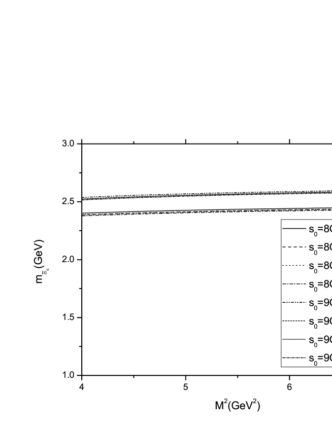
Figure 1: The mass of the $\Xi_{c}$ as a function of the Borel parameter $M^{2}$ for different values of arbitrary parameter $\beta$ and the continuum threshold $s_{0}$.

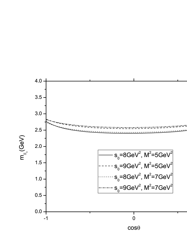
Figure 2: The dependence of the mass of the $\Xi_{c}$ on $\cos\theta$ for different values of Borel parameter $M^{2}$ and the continuum threshold $s_{0}$.

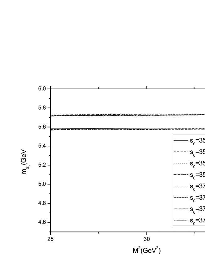
Figure 3: The mass of the $\Xi_{b}$ as a function of the Borel parameter $M^{2}$ for different values of arbitrary parameter $\beta$ and the continuum threshold $s_{0}$.

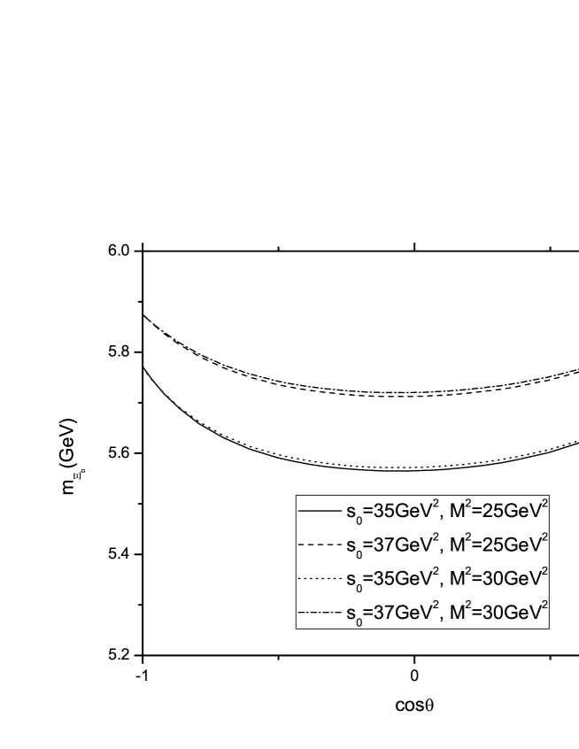
Figure 4: The dependence of the mass of the $\Xi_{b}$ on $\cos\theta$ for different values of Borel parameter $M^{2}$ and the continuum threshold $s_{0}$.

Looking at the result of LCQCD sum rules calculation for the coupling constant $g_{\Xi_{Q}\Xi_{Q}\pi}$ one encounters three auxiliary parameters. These parameters are the Borel mass $M^{2}$, the continuum threshold $s_{0}$ and the arbitrary parameter $\beta$ and there should be no dependency of a physical quantity, such as the coupling constant for our case, on them. Therefore at this stage a working region of these auxiliary parameters should be determined. In order to determine the upper and lower bound of $M$ we use the requirements that the continuum contribution be less than that of the ground state, and the highest power of $1/M^{2}$ be less than $30^{0}/_{0}$ of the highest power of $M$. The former (latter) is used to determine upper (lower) bound of $M^{2}$. To determine the value of continuum threshold $s_{0}$ we use the two-point correlation function from which we obtain the mass sum rules. In Fig. 1 and Fig. 2, we plot the dependence of our prediction on $m_{\Xi_{c}}$ to the Borel parameter $M^{2}$, and $\cos\theta$, where $\beta=\cos\theta$, respectively. For these plots, the continuum threshold is chosen to be $s_{0}=8$ Gev² and $s_{0}=9$ Gev². For these values of the continuum threshold we see from these figures that our predictions are in agreement with experimental results and that there is no dependence on the auxiliary parameters. In Figs. 3, 4, we carry out the same analysis for $m_{\Xi_{b}}$ and find the continuum threshold to be $s_{0}=36$ Gev² and $s_{0}=37$ Gev². In Fig. 4, we also observe that our prediction is stable with respect to variations of $\theta$ for the region $0.5<\cos\theta<0.5$ which corresponds to $|\beta|>1.7$.

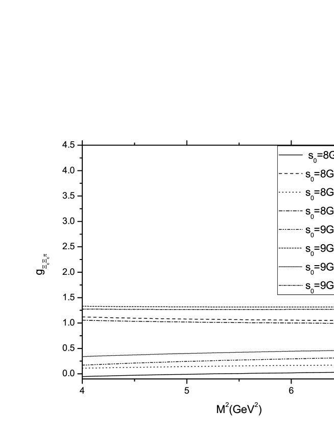
Figure 5: The dependence of the coupling constant $g_{{\Xi_{c}\Xi_{c}\pi}}$ on the Borel parameter $M^{2}$ for different values arbitrary parameter $\beta$ and the continuum threshold $s_{0}$.

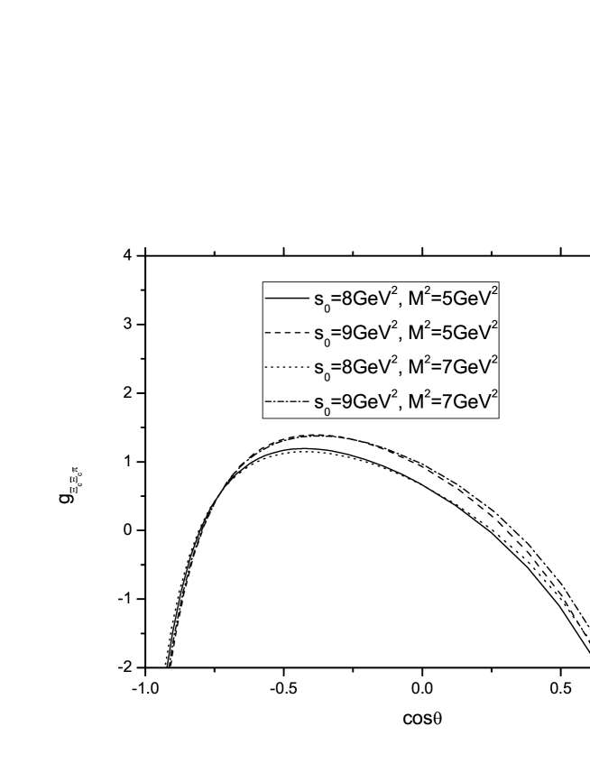
Figure 6: The dependence of the coupling constant $g_{{\Xi_{c}\Xi_{c}\pi}}$ on $\cos\theta$ for different values of Borel parameter $M^{2}$ and the continuum threshold $s_{0}$.

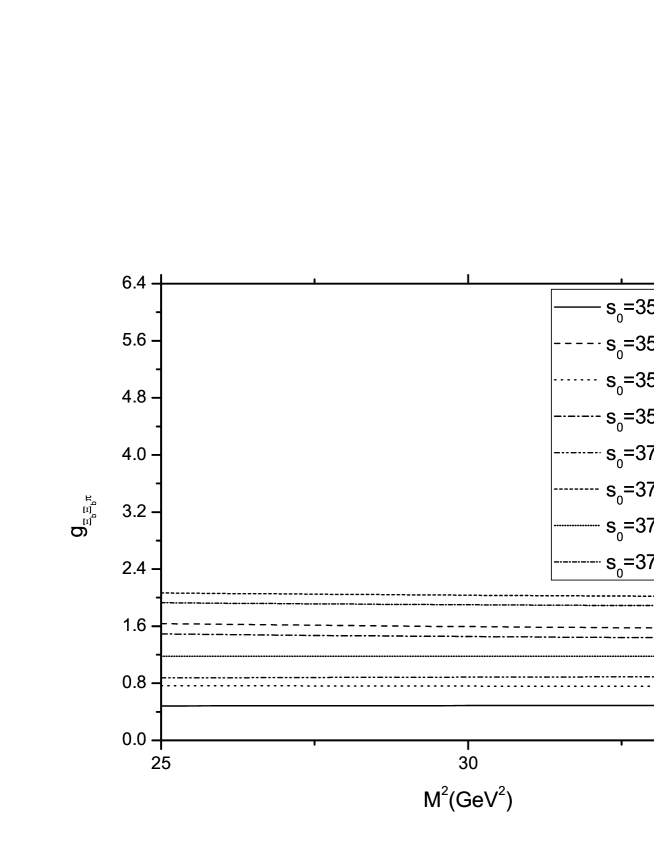
Figure 7: The dependence of the coupling constant $g_{{\Xi_{b}\Xi_{b}\pi}}$ on the Borel parameter $M^{2}$ for different values of arbitrary parameter $\beta$ and the continuum threshold $s_{0}$.

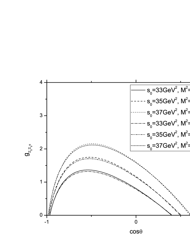
Figure 8: The dependence of the coupling constant $g_{{\Xi_{b}\Xi_{b}\pi}}$ on $\cos\theta$ for different values of Borel parameter $M^{2}$ and the continuum threshold $s_{0}$.

The results for the coupling constant calculation are presented in Figs. 5, 6, 7 and 8. Figs. 5 and 7 depicts respectively the dependence of the coupling constants $g_{\Xi_{c}\Xi_{c}\pi}$ and $g_{\Xi_{b}\Xi_{b}\pi}$ on $M^{2}$ in the working region of $M^{2}$. The results are given for two fixed values of $\beta$ and two fixed values of $s_{0}$ for each coupling constant. It follows from the figures that the results are rather stable with respect to the variations of $M^{2}$ in the given region of $M^{2}$. The dependence of the coupling constants on $\cos\theta$ are also presented in Figs. 6 and 8 and with respect to these figures when $\cos\theta$ is in between $-0.25<\cos\theta<0.25$ the coupling constant $g_{\Xi_{c}\Xi_{c}\pi}$ is practically independent of the unphysical parameter $\beta$. The interval of $\beta$ that gives coupling constant result independent of $\beta$ for $g_{\Xi_{b}\Xi_{b}\pi}$ is $-0.75<\cos\theta<0.75$. As a result of our analysis we obtain the values of the coupling constants as

$$g_{\Xi_{c}\Xi_{c}\pi}=1.0\pm 0.5,~{}~{}~{}~{}~{}~{}~{}~{}~{}~{}~{}~{}~{}~{}~{}g_{\Xi_{b}\Xi_{b}\pi}=1.6\pm 0.4.$$

To summarize, in this work we present the results of the coupling constant for the coupling constants $g_{\Xi_{c}\Xi_{c}\pi}$ and $g_{\Xi_{b}\Xi_{b}\pi}$. To this end, we make use of the LCQSR approach with the $\Xi_{Q}$ current applied in its most general form. We obtain the appropriate values of the threshold parameters $s_{0}$ from the mass sum rules and, using them and appropriate intervals of Borel parameter and $\beta$, we attain the coupling constants $g_{\Xi_{c}\Xi_{c}\pi}$ and $g_{\Xi_{b}\Xi_{b}\pi}$.

IV Acknowledgment

The authors would like to thank T. M. Aliev for his useful discussions. S. H. L. was supported by the Korean Research Foundation KRF-2006-C00011. The work of A. O. and Y. S. have been supported in part by the European Union (HadronPhysics2 project ”Study of strongly interacting matter”).

Appendix A

$$\rho(s) = -\frac{f_{\pi}m_{Q}^{2}}{768\sqrt{2}\pi^{2}}\Bigg{[}3m_{b}\Bigg{\{}m_{Q}(1+6\beta+\beta^{2})(2\psi_{10}-\psi_{20}+\psi_{30})-4m_{Q}(3-4\beta+\beta^{2})\psi_{10}$$

$$-2[m_{Q}(1+6\beta+\beta^{2})\psi_{00}-2m_{s}(3-4\beta+\beta^{2})]ln(\frac{s}{m_{Q}^{2}})\Bigg{\}}+u_{0}^{2}m_{\pi}^{2}8(1+7\beta+\beta^{2})\psi_{32}\Bigg{]}\varphi_{\pi}(u_{0})$$

$$-\frac{\mu_{\pi}}{384\sqrt{2}\pi^{2}}(\beta-1)(\widetilde{\mu}^{2}-1)\Bigg{[}2m_{Q}^{2}[(-m_{Q}+3\beta m_{Q}+5m_{s}+3\beta m_{s})\psi_{10}+m_{Q}(1-3\beta)ln(\frac{s}{m_{Q}^{2}})]$$

$$-[m_{Q}(3\beta-1)(2\psi_{10}-\psi_{11}-\psi_{12}+2\psi_{21})+m_{s}(5+3\beta)(\psi_{11}+\psi_{12})]u_{0}m_{\pi}^{2}\Bigg{]}\varphi_{\sigma}(u_{0})$$

$$-\frac{f_{\pi}m_{\pi}^{2}}{256\sqrt{2}\pi^{2}}\Bigg{[}-m_{Q}\Bigg{\{}m_{Q}(1+6\beta+\beta^{2})\psi_{10}+m_{s}(3-4\beta+\beta^{2})\psi_{00}\Bigg{\}}$$

$$+2(1+7\beta+\beta^{2})(\psi_{11}+\psi_{12})u_{0}^{2}m_{\pi}^{2}\Bigg{]}A(u_{0})-\frac{f_{\pi}m_{Q}^{4}u_{0}}{384\sqrt{2}\pi^{2}}[1+7\beta+\beta^{2})\Bigg{[}6\psi_{10}-3\psi_{20}+\psi_{30}-2\psi_{41}$$

$$-6\psi_{00}ln(\frac{s}{m_{Q}^{2}})\Bigg{]}\varphi_{\pi}^{\prime}(u_{0})-\frac{\mu_{\pi}m_{Q}^{2}u_{0}}{768\sqrt{2}\pi^{2}}(\beta-1)(\widetilde{\mu}^{2}-1)\Bigg{[}m_{Q}(3\beta-1)(2\psi_{10}-\psi_{20}+\psi_{31})$$

$$+m_{s}(5+3\beta)(\psi_{20}-\psi_{31})+2m_{Q}(1-3\beta)ln(\frac{s}{m_{Q}^{2}})\Bigg{]}\varphi_{\sigma}^{\prime}(u_{0})-\frac{f_{\pi}m_{\pi}^{2}m_{Q}^{2}u_{0}}{256\sqrt{2}\pi^{2}}(1+7\beta+\beta^{2})(\psi_{20}-\psi_{31})A^{\prime}(u_{0})$$

$$-\frac{f_{\pi}\mu_{\pi}}{64\sqrt{2}\pi^{2}m_{Q}}\Bigg{[}m_{s}(-1-4\beta+5\beta^{2})[m_{Q}^{2}(-1+3\psi_{00}-\psi_{01}+\psi_{10})-s\psi_{00}](\eta_{1}-2\eta_{2})ln(\frac{\Lambda^{2}}{m_{Q}})$$

$$+m_{Q}^{2}\mu_{\pi}\Bigg{\{}m_{s}(-1-4\beta+5\beta^{2})\psi_{01}(\eta_{1}-2\eta_{2})ln(\frac{s}{\Lambda^{2}})+[m_{Q}u_{0}(2+14\beta+2\beta^{2})(2\eta^{\prime}_{4}-\eta^{\prime}_{3})$$

$$-(5+14\beta+5\beta^{2})(2\eta^{\prime}_{8}-\eta_{7})+m_{Q}(7-2\beta+7\beta^{2})\eta_{1}+m_{s}(-5+4\beta+\beta^{2})(\eta_{1}-2\eta_{2})]ln(\frac{s}{m_{Q}^{2}})$$

$$+m_{s}(-1-4\beta+5\beta^{2})(\eta_{1}-2\eta_{2})\Bigg{(}\gamma_{E}(2\psi_{00}-\psi_{10}+\psi_{11}-\psi_{21})+(-2\psi_{00}+\psi_{01}+\psi_{10}-\psi_{21})ln(\frac{s-m_{Q}^{2}}{\Lambda^{2}})$$

$$-\psi_{00}ln(\frac{m_{Q}^{2}(s-m_{Q}^{2})}{\Lambda^{2}s})\Bigg{)}\Bigg{\}}-[m_{Q}^{4}(1-4\beta+3\beta^{2})+m_{Q}^{3}m_{s}(-5+2\beta+3\beta^{2})](2\eta^{\prime}_{6}-\eta^{\prime}_{5})ln(\frac{s}{m_{Q}^{2}})\Bigg{]}$$

$$+\frac{1}{128\sqrt{2}\pi^{2}}\Bigg{[}f_{\pi}m_{\pi}^{2}\mu_{\pi}\Bigg{\{}2m_{Q}\Bigg{(}3m_{Q}u_{0}(1+\beta^{2})(\psi_{20}-\psi_{31})(2\eta^{\prime}_{8}-\eta^{\prime}_{7})+m_{Q}(1+\beta^{2})[(2\eta^{\prime}_{8}-\eta_{7}^{\prime}-10\eta^{\prime}_{4}+5\eta^{\prime}_{3})$$

$$+14(1+\beta^{2})m_{Q}\eta_{1}-m_{s}(1-5\beta^{2})(\eta_{1}-2\eta_{2})]\psi_{10}+m_{Q}(1-5\beta^{2})(\psi_{00}-\psi_{01}-\psi_{21})(\eta_{1}-2\eta_{2})\Bigg{)}$$

$$+3m_{Q}u_{0}[m_{Q}(\psi_{20}-\psi_{31})-2m_{s}(\psi_{10}+\psi_{21})]\zeta+m_{Q}u_{0}\beta^{2}[3m_{Q}(\psi_{20}-\psi_{31})-2m_{s}(\psi_{10}+\psi_{21})]\zeta$$

$$-2u_{0}^{2}m_{\pi}^{2}(1+\beta^{2})[(12\psi_{10}-3\psi_{11}-3\psi_{12}+12\psi_{21})\eta_{1}+(-10\psi_{10}+6\psi_{11}+6\psi_{12}-10\psi_{21})\eta_{2}]\Bigg{\}}$$

$$+2\mu_{\pi}[(m_{Q}-5m_{s})+3\beta^{2}(m_{Q}+m_{s})][(2\eta^{\prime}_{6}-\eta^{\prime}_{5})\psi_{10}+2u_{0}m_{\pi}^{2}(\psi_{10}+\psi_{21})(2\eta_{6}-\eta_{5})]\Bigg{]}$$

$$+\frac{\beta}{64\sqrt{2}\pi^{2}}\Bigg{[}f_{\pi}m_{\pi}^{2}2m_{Q}\Bigg{\{}[7m_{q}u_{0}(2\eta^{\prime}_{4}-\eta^{\prime}_{3}+\eta^{\prime}_{7}-2\eta^{\prime}_{8})+4m_{Q}\eta_{1}$$

$$-2m_{s}(\eta_{1}-2\eta_{2})]\psi_{10}+2m_{s}(\psi_{00}-\psi_{01}-\psi_{21})(\eta_{1}-2\eta_{2})+m_{Q}u_{0}[11m_{Q}(\psi_{20}-\psi_{31})+4m_{s}(\psi_{10}+\psi_{21})]\zeta$$

$$-2u_{0}^{2}m_{\pi}^{2}[(6\psi_{10}+3\psi_{11}+3\psi_{12}+6\psi_{21})\eta_{1}-14(\psi_{10}+\psi_{21})\eta_{2}]\Bigg{\}}+2\mu_{\pi}\Bigg{\{}(2m_{q}-m_{s})[m_{Q}^{2}(2\eta^{\prime}_{6}-\eta^{\prime}_{5})$$

$$+2u_{0}m_{\pi}^{2}(\psi_{10}+\psi_{21})(2\eta_{6}-\eta_{5})]\Bigg{\}}\Bigg{]}+\frac{\langle\bar{s}s\rangle}{288\sqrt{2}}\Bigg{[}3f_{\pi}\Bigg{\{}2m_{Q}(3-4\beta+\beta^{2})-m_{s}(1+6\beta+\beta^{2})\Bigg{\}}\varphi_{\pi}(u_{0})$$

$$+2\mu_{\pi}\Bigg{\{}(-5+2\beta+3\beta^{2})(\widetilde{\mu}_{\pi}^{2}-1)\psi_{00}\Bigg{\}}\varphi_{\sigma}(u_{0})+6f_{\pi}u_{0}\Bigg{\{}(1+7\beta+\beta^{2})\psi_{00}\Bigg{\}}\varphi_{\pi}^{\prime}(u_{0})\$$

$$+\mu_{\pi}u_{0}\Bigg{\{}(-5+2\beta+3\beta^{2})(\widetilde{\mu}_{\pi}^{2}-1)\psi_{00}\Bigg{\}}\varphi_{\sigma}^{\prime}(u_{0})-6(1+\gamma_{E})\mu_{\pi}(-5+2\beta+3\beta^{2})(2\eta^{\prime}_{6}-\eta^{\prime}_{5})\psi_{00}\Bigg{]}$$

$$+\frac{\langle g_{s}^{2}G^{2}\rangle}{4608\sqrt{2}\pi^{2}}\Bigg{[}f_{\pi}\Bigg{\{}\frac{-6m_{Q}^{3}m_{s}}{M^{2}}(3-4\beta+\beta^{2})ln(\frac{s-m_{Q}^{2}}{\Lambda^{2}})\psi_{00}+\frac{1}{m_{Q}^{2}}[-m_{Q}(1+6\beta+\beta^{2})$$

$$+2m_{s}(1-9\gamma_{E})(3-4\beta+\beta^{2})]\psi_{00}+18m_{Q}m_{s}(3-4\beta+\beta^{2})(\psi_{00}-\psi_{02}-2\psi_{10}+2\psi_{21}\psi_{22})ln(\frac{s-m_{Q}^{2}}{\Lambda^{2}})$$

$$+4u_{0}^{2}m_{\pi}^{2}(1+7\beta+\beta^{2})\psi_{02}\Bigg{\}}\varphi_{\pi}(u_{0})+\Bigg{\{}\frac{\mu_{\pi}m_{s}(\tilde{\mu}_{\pi}^{2}-1)}{M^{2}}(-5+2\beta+3\beta^{2})ln(\frac{s-m_{Q}^{2}}{\Lambda^{2}})\psi_{10}[u_{0}^{2}m_{\pi}^{2}(-\frac{3}{M^{2}}-\frac{2}{m_{Q}^{2}}$$

$$-\frac{2m_{Q}^{2}}{M^{4}})+\frac{2m_{Q}^{2}}{M^{4}}]-\frac{\mu_{\pi}(\beta-1)(\tilde{\mu}_{\pi}^{2}-1)}{6m_{Q}^{6}}\Bigg{(}m_{Q}^{4}\Big{[}4m_{Q}(3\beta-1)\psi_{00}-3m_{s}(5+3\beta)(56\gamma_{E}\psi_{00}-\psi_{20}+\psi_{21}+\psi_{31})$$

$$+12m_{s}(5+3\beta)(14\psi_{00}-14\psi_{03}-42\psi_{10}+30\psi_{20}+27\psi_{21}+18\psi_{22}+9\psi_{23}+24\psi_{31}+12\psi_{32})ln(\frac{s-m_{Q}^{2}}{\Lambda^{2}})\Big{]}$$

$$-6u_{0}^{2}m_{\pi}^{2}\Big{[}m_{Q}^{2}[m_{Q}(3\beta-1)\psi_{02}+m_{s}(5+3\beta)(-61\psi_{00}+20\psi_{01}+20\psi_{02}+20\psi_{03}+122\psi_{10}+2\psi_{12}+5\psi_{13}+11\psi_{14}$$

$$-122\psi_{21}-61\psi_{22}-20\psi_{23})]+6m_{s}(5+3\beta)\{[m_{Q}^{2}(39\psi_{00}+40\psi_{10})-40s\psi_{00}]ln(\frac{s-m_{Q}^{2}}{\Lambda^{2}})$$

$$+m_{Q}^{2}\psi_{04}ln(\frac{s(s-m_{Q}^{2})}{m_{Q}^{2}\Lambda^{2}})\}\Big{]}\Bigg{)}\Bigg{\}}\varphi_{\sigma}(u_{0})+(3-4\beta+\beta^{2})f_{\pi}m_{\pi}^{2}m_{s}\Bigg{\{}(\frac{3m_{Q}^{5}}{2M^{8}}-\frac{3m_{Q}^{3}}{4M^{6}})ln(\frac{s-m_{Q}^{2}}{\Lambda^{2}})$$

$$+18\frac{1}{m_{Q}^{3}}[2\psi_{00}-\psi_{01}-\psi_{02}-3\psi_{10}+3\psi_{21}+\psi_{22}+2(\psi_{00}-\psi_{03}-3\psi_{10}+3\psi_{21}+2\psi_{22}+\psi_{23})ln(\frac{s-m_{Q}^{2}}{\Lambda^{2}})]\Bigg{\}}A(u_{0})$$

$$-2(1+7\beta+\beta^{2})f_{\pi}u_{0}(\psi_{10}+\psi_{21})\varphi_{\pi}^{\prime}(u_{0})+\Bigg{\{}\frac{(-5+2\beta+3\beta^{2})}{M^{2}}m_{s}u_{0}\mu_{\pi}(\tilde{\mu}_{\pi}^{2}-1)(\frac{m_{Q}^{2}}{M^{2}}+\frac{3}{2})ln(\frac{s-m_{Q}^{2}}{\Lambda^{2}})\psi_{00}$$

$$+\frac{1}{6m_{Q}^{2}}(\beta-1)(\tilde{\mu}_{\pi}^{2}-1)\Bigg{(}(3\beta-1)m_{Q}(\psi_{00}-3\psi_{10}-3\psi_{21})+3m_{s}(5+3\beta)[(20\gamma_{E}-1)\psi_{00}+\psi_{10}-2\psi_{12}-\psi_{20}+\psi_{31}]$$

$$+12m_{s}(5+3\beta)(5\psi_{00}-5\psi_{03}-15\psi_{10}+30\psi_{20}+24\psi_{31}+12\psi_{32}+4\psi_{33})ln(\frac{s-m_{Q}^{2}}{\Lambda^{2}})\Bigg{)}\Bigg{\}}\varphi_{\sigma}^{\prime}(u_{0})$$

$$+\frac{1}{M^{4}}(\beta-1)m_{Q}m_{s}\Bigg{\{}3f_{\pi}m_{\pi}^{2}(7\beta-13)(\eta_{1}-2\eta_{2})-m_{Q}\mu_{\pi}(10+6\beta)(2\eta^{\prime}_{6}-\eta^{\prime}_{5})-\frac{2m_{Q}}{M^{2}}\mu_{\pi}^{2}[m_{Q}f_{\pi}(2\beta-14)(\eta_{1}-2\eta_{2})$$

$$-u_{0}(3\beta-9)\zeta]+6u_{0}(5+3\beta)(2\eta_{6}-\eta_{5})\Bigg{\}}ln(\frac{s-m_{Q}^{2}}{\Lambda^{2}})-\frac{2}{m_{Q}^{4}}(\beta-1)\Bigg{\{}3m_{Q}m_{s}f_{\pi}\mu_{\pi}^{2}\Bigg{(}(18-6\beta)u_{0}\zeta[2\psi_{00}-\psi_{01}$$

$$-\psi_{02}-3\psi_{10}+3\psi_{21}+\psi_{22}+2(\psi_{00}-\psi_{03}-3\psi_{10}+3\psi_{21}+2\psi_{22}+\psi_{23})ln(\frac{s-m_{Q}^{2}}{\Lambda^{2}})]+(\eta_{1}-2\eta_{2})\Big{[}(1+5\beta)\gamma_{E}\psi_{00}$$

$$+(15+5\beta)(\psi_{10}-\psi_{11}-\psi_{21})-(\psi_{00}+3\psi_{02}-4\psi_{03}-36\psi_{10}+15\psi_{11}+15\psi_{12}+36\psi_{21}+20\psi_{22}+4\psi_{23}$$

$$+\beta[5\psi_{00}+15\psi_{02}-20\psi_{03}-36\psi_{10}+3\psi_{11}+3\psi_{12}+36\psi_{21}+28\psi_{22}+20\psi_{23}])ln(\frac{s-m_{Q}^{2}}{\Lambda^{2}})\Big{]}\Bigg{)}$$

$$+\mu_{\pi}\Bigg{(}m_{Q}^{2}(\eta^{\prime}_{5}-2\eta^{\prime}_{6})\Big{[}m_{Q}(3\beta-1)\psi_{00}-18m_{s}(5+3\beta)[\gamma_{E}\psi_{00}-(\psi_{00}-\psi_{02}-2\psi_{10}+3\psi_{20}+3\psi_{31}+\psi_{32})ln(\frac{s-m_{Q}^{2}}{\Lambda^{2}})]\Big{]}$$

$$-36m_{\pi}^{2}m_{s}u_{0}(5+3\beta)(\eta_{5}-2\eta_{6})\Big{[}2\psi_{00}-\psi_{01}-\psi_{02}-3\psi_{10}+3\psi_{21}+\psi_{22}+2(\psi_{00}-\psi_{03}-3\psi_{10}+3\psi_{21}+2\psi_{22}$$

$$+\psi_{23})ln(\frac{s-m_{Q}^{2}}{\Lambda^{2}})\Big{]}\Bigg{)}\Bigg{\}}\Bigg{]},$$ (16)

and

$$\Gamma = \frac{f_{\pi}m_{\pi}^{2}}{32\sqrt{2}\pi^{2}}m_{Q}m_{s}\gamma_{E}M^{2}(-1+4\beta+5\beta^{2})(\eta_{1}-2\eta_{2})+\frac{\langle\bar{s}s\rangle}{1728\sqrt{2}}\Bigg{[}f_{\pi}\Bigg{\{}\frac{3}{M^{4}}m_{0}^{2}m_{Q}^{2}m_{s}[m_{Q}^{2}(1+6\beta+\beta^{2})$$

$$-4u_{0}^{2}m_{\pi}^{2}(1+7\beta+\beta^{2})]+6m_{Q}[m_{0}^{2}(\beta^{2}-1)+3m_{Q}m_{s}(1+6\beta+\beta^{2})]-72m_{s}u_{0}^{2}m_{\pi}^{2}(1+7\beta+\beta^{2})$$

$$+\frac{m_{0}^{2}}{M^{2}}[9m_{Q}^{3}(3-4\beta+\beta^{2})+m_{Q}^{2}m_{s}(-11+10\beta-11\beta^{2})+2m_{s}u_{0}^{2}m_{\pi}^{2}(13+46\beta+13\beta^{2})]\Bigg{\}}\varphi_{\pi}(u_{0})$$

$$+\mu_{\pi}(\tilde{\mu}_{\pi}^{2}-1)\Bigg{\{}12(-5+2\beta+3\beta^{2})(m_{Q}^{2}-u_{0}^{2}m_{\pi}^{2})+\frac{1}{M^{2}}(\beta-1)\Bigg{(}\frac{m_{0}^{2}m_{Q}^{3}m_{s}}{M^{4}}(3\beta-1)(m_{Q}^{2}-u_{0}^{2}m_{\pi})$$

$$-\frac{m_{0}^{2}m_{Q}}{M^{2}}[m_{Q}^{4}(15+9\beta)+m_{Q}^{2}m_{s}(7\beta-5)-m_{Q}u_{0}^{2}m_{\pi}^{2}(15+3\beta)-m_{s}u_{0}^{2}m_{\pi}^{2}(\beta-3)]-6m_{Q}^{3}m_{s}(3\beta-1)$$

$$-m_{Q}^{2}m_{0}^{2}(\beta-1)+m_{Q}m_{0}^{2}m_{s}(\beta-3)+2u_{0}^{2}m_{\pi}^{2}[m_{0}^{2}(5+7\beta)+m_{Q}m_{s}(9\beta-3)]\Bigg{)}\Bigg{\}}\varphi_{\sigma}(u_{0})$$

$$+\frac{m_{\pi}^{2}f_{\pi}}{M^{2}}\Bigg{\{}\frac{3m_{0}^{2}m_{Q}^{4}m_{s}}{4M^{6}}[m_{Q}^{2}(1+6\beta+\beta^{2})-4u_{0}^{2}m_{\pi}^{2}(1+7\beta+\beta^{2})]+\frac{3}{2}[m_{Q}m_{0}^{2}(\beta^{2}-1)+6m_{Q}^{3}(3-4\beta+\beta^{2})$$

$$+12m_{s}u_{0}^{2}m_{\pi}^{2}(1+7\beta+\beta^{2})]+\frac{m_{Q}^{2}}{2M^{2}}[-9m_{Q}^{2}m_{s}(1+6\beta+\beta^{2})+6m_{0}^{2}m_{Q}(5-6\beta+\beta^{2})m_{0}^{2}m_{s}(-11+10\beta-11\beta^{2})$$

$$+36m_{s}u_{0}^{2}m_{\pi}^{2}(1+7\beta+\beta^{2})]+\frac{m_{Q}^{2}m_{0}^{2}}{4M^{4}}[-9m_{Q}^{3}(3-4\beta+\beta^{2})+2m_{Q}^{2}m_{s}(1-32\beta+\beta^{2})$$

$$-2m_{s}u_{0}^{2}m_{\pi}^{2}(7+4\beta+7\beta^{2})]\Bigg{\}}A(u_{0})-m_{0}^{2}m_{s}u_{0}f_{\pi}\Bigg{\{}(13+46\beta+13\beta^{2})+6\frac{m_{Q}^{2}}{M^{2}}(1+7\beta+\beta^{2})\Bigg{\}}\varphi_{\pi}^{\prime}(u_{0})$$

$$+\mu_{\pi}(\tilde{\mu}_{\pi}^{2}-1)u_{0}(\beta-1)\Bigg{\{}-m_{0}^{2}(7+5\beta)-3m_{Q}m_{s}(3\beta-1)+\frac{m_{0}^{2}m_{Q}^{3}m_{s}}{2M^{4}}(3\beta-1)$$

$$-\frac{m_{0}^{2}m_{Q}}{2M^{2}}[3m_{Q}(5+3\beta)+m_{s}(\beta-3)]\Bigg{\}}\varphi_{\sigma}^{\prime}(u_{0})+m_{s}u_{0}f_{\pi}m_{\pi}^{2}\Bigg{\{}-9(1+7\beta+\beta^{2})(1+\frac{m_{Q}^{2}}{M^{2}}-\frac{m_{0}^{2}m_{Q}^{4}}{6M^{6}})$$

$$+\frac{4m_{0}^{2}m_{Q}^{2}}{M^{4}}(7+4\beta+7\beta^{2})\Bigg{\}}A^{\prime}(u_{0})-\frac{3m_{0}^{2}m_{Q}^{2}m_{s}f_{\pi}m_{\pi}^{2}}{M^{6}}\Bigg{\{}m_{Q}^{2}[(7-2\beta+7\beta^{2})\eta_{1}+u_{0}(3+22\beta+3\beta^{2})\zeta]$$

$$-u_{0}^{2}m_{\pi}^{2}[6(1+\beta+\beta^{2})\eta_{1}-(5+14\beta+5\beta^{2})\eta_{2}]\Bigg{\}}+\frac{3}{M^{2}}\Bigg{\{}f_{\pi}m_{\pi}^{2}\Bigg{(}m_{Q}m_{0}^{2}[3(-5+4\beta+\beta^{2})(\eta_{1}-2\eta_{2})$$

$$-2u_{0}(\beta^{2}-1)\zeta]+6m_{Q}^{2}m_{s}[(7-2\beta+7\beta^{2})\eta_{1}+u_{0}(3+22\beta+3\beta^{2})\zeta]-12m_{Q}m_{s}u_{0}^{2}m_{\pi}^{2}[6(1+\beta+\beta^{2})\eta_{1}$$

$$-(5+14\beta+5\beta^{2})\eta_{2}]\Bigg{)}+3m_{0}^{2}m_{Q}^{2}\mu_{\pi}(-5+2\beta+3\beta^{2})(2\eta^{\prime}_{6}-\eta^{\prime}_{5})\Bigg{\}}$$

$$-\frac{3m_{0}^{2}m_{Q}^{2}m_{\pi}^{2}}{M^{4}}\Bigg{\{}f_{\pi}\Bigg{(}3m_{Q}(-5+4\beta+\beta^{2})(\eta_{1}-2\eta_{2})+3m_{Q}u_{0}(3-4\beta+\beta^{2})\zeta+2m_{s}u_{0}(1+7\beta+\beta^{2})(2\eta^{\prime}_{4}-\eta^{\prime}_{3})$$

$$-m_{s}(5+14\beta+5\beta^{2})\eta^{\prime}_{7}-2m_{s}(7-2\beta+7\beta^{2})\eta_{1}+m_{s}u_{0}(1+6\beta+\beta^{2})\zeta\Bigg{)}-6u_{0}\mu_{\pi}(-5+2\beta+3\beta^{2})(2\eta_{6}-\eta_{5})\Bigg{\}}$$

$$+18m_{\pi}^{2}\Bigg{\{}f_{\pi}\Bigg{(}2m_{s}u_{0}(1+7\beta+\beta^{2})(2\eta^{\prime}_{4}-\eta^{\prime}_{3})-m_{s}u_{0}(5+14\beta+5\beta^{2})\eta^{\prime}_{7}+m_{s}u_{0}(3+22\beta+3\beta^{2})\zeta$$

$$+2m_{Q}(-5+4\beta+\beta^{2})(\eta_{1}-2\eta_{2})+2m_{Q}u_{0}(3-4\beta+\beta^{2})\zeta\Bigg{)}-4u_{0}\mu_{\pi}(-5+2\beta+3\beta^{2})(2\eta_{6}-\eta_{5})\Bigg{\}}\Bigg{]}$$

$$+\frac{\langle g^{2}G^{2}\rangle}{4608\sqrt{2}\pi^{2}}\Bigg{[}m_{s}f_{\pi}(3-4\beta+\beta^{2})\Bigg{\{}m_{Q}+\frac{18\gamma_{E}M^{2}}{m_{Q}}-\frac{m_{Q}^{3}}{M^{2}}[2+3ln(\frac{\Lambda^{2}}{m_{Q}^{2}})]\Bigg{\}}\varphi_{\pi}(u_{0})$$

$$+\mu_{\pi}(\tilde{\mu}\pi^{2}-1)\Bigg{\{}m_{s}(-5+2\beta+3\beta^{2})\Bigg{(}-\frac{4M^{2}\gamma_{E}}{m_{Q}^{2}}+\frac{m_{Q}^{2}}{3M^{4}}[2+3ln(\frac{\Lambda^{2}}{m_{Q}^{2}})](m_{Q}^{2}-u_{0}^{2}m_{\pi}^{2})+\frac{1}{3M^{2}}[10m_{Q}^{2}-6u_{0}^{2}m_{\pi}^{2}$$

$$-3u_{0}^{2}m_{\pi}^{2}\gamma_{E}-6u_{0}^{2}m_{\pi}^{2}ln(\frac{\Lambda^{2}}{m_{Q}^{2}})]\Bigg{)}+\frac{(\beta-1)}{3m_{Q}^{2}}\Bigg{(}m_{Q}^{2}[m_{Q}(3\beta-1)+9m_{s}(5+3\beta)]-u_{0}^{2}m_{\pi}^{2}[m_{Q}(3\beta-1)\$$

$$+6m_{s}(5+3\beta)(1+2\gamma_{E})+6m_{s}(5+3\beta)ln(\frac{\Lambda^{2}}{m_{Q}^{2}})]\Bigg{)}\Bigg{\}}\varphi_{\sigma}(u_{0})+f_{\pi}m_{\pi}^{2}\Bigg{\{}m_{s}(3-4\beta+\beta^{2})\Bigg{(}-\frac{3}{4m_{Q}}$$

$$+\frac{m_{Q}^{5}}{4M^{6}}[2+3ln(\frac{\Lambda^{2}}{m_{Q}^{2}})]-\frac{3m_{Q}^{3}}{4M^{4}}[-3+\gamma_{E}+3ln(\frac{\Lambda^{2}}{m_{Q}^{2}})]\Bigg{)}+\frac{1}{4M^{2}}[m_{Q}^{2}(1+6\beta+\beta^{2})-12m_{Q}m_{s}(3-4\beta+\beta^{2})$$

$$-4u_{0}^{2}m_{\pi}^{2}(1+7\beta+\beta^{2})]\Bigg{\}}A(u_{0})+m_{s}u_{0}\mu_{\pi}(\tilde{\mu}_{\pi}^{2}-1)(-5+2\beta+3\beta^{2})\Bigg{\{}-\frac{10M^{2}\gamma_{E}}{m_{Q}^{2}}+1+2\gamma_{E}+ln(\frac{\Lambda^{2}}{m_{Q}^{2}})$$

$$+\frac{m_{Q}^{2}}{6M^{2}}[2+3ln(\frac{\Lambda^{2}}{m_{Q}^{2}})]\Bigg{\}}\varphi_{\sigma}^{\prime}(u_{0})+\frac{f_{\pi}m_{\pi}^{2}u_{0}}{2}(1+7\beta+\beta^{2})A^{\prime}(u_{0})+\frac{6m_{s}M^{2}\gamma_{E}}{m_{Q}^{3}}\Bigg{\{}f_{\pi}m_{\pi}^{2}(-1-4\beta+5\beta^{2})(\eta_{1}-2\eta_{2})$$

$$+6m_{Q}\mu_{\pi}(-5+2\beta+3\beta^{2})(2\eta^{\prime}_{6}-\eta^{\prime}_{5})\Bigg{\}}+\frac{m_{Q}^{2}m_{s}m_{\pi}^{2}}{M^{4}}(\beta-1)\Bigg{\{}m_{Q}f_{\pi}\Bigg{(}u_{0}(3-\beta)[2+3ln(\frac{\Lambda^{2}}{m_{Q}^{2}})]\zeta$$

$$+2[-5-\beta+(\beta-7)ln(\frac{\Lambda^{2}}{m_{Q}^{2}})](\eta_{1}-2\eta_{2})\Bigg{)}+2\mu_{\pi}u_{0}(5+3\beta)[2+3ln(\frac{\Lambda^{2}}{m_{Q}^{2}})](2\eta_{10}-\eta_{9})\Bigg{\}}$$

$$+\frac{1}{M^{2}}\Bigg{\{}m_{Q}f_{\pi}m_{\pi}^{2}\Bigg{(}-m_{Q}(7+10\beta+7\beta^{2})\eta_{1}-m_{s}[8(4-5\beta+\beta^{2})-3(-5+4\beta+\beta^{2})\gamma_{E}(\eta_{1}-2\eta_{2})$$

$$-7u_{0}(3-4\beta+\beta^{2})\zeta]+9m_{s}(3-4\beta+\beta^{2})(\eta_{1}-2\eta_{2})ln(\frac{\Lambda^{2}}{m_{Q}^{2}})\Bigg{)}+2u_{0}^{2}f_{\pi}m_{\pi}^{4}[3(1+4\beta+\beta^{2})\eta_{1}+(1-14\beta+\beta^{2})\eta_{2}]$$

$$+m_{Q}^{2}m_{s}\mu_{\pi}(-5+2\beta+3\beta^{2})[2+3ln(\frac{\Lambda^{2}}{m_{Q}^{2}})](\eta^{\prime}_{5}-2\eta^{\prime}_{6})+2u_{0}m_{\pi}^{2}\mu_{\pi}[m_{Q}(-1+4\beta-3\beta^{2})$$

$$-6m_{s}(-5+2\beta+3\beta^{2})](2\eta_{6}-\eta_{5})\Bigg{\}}+\frac{1}{m_{Q}^{2}}\Bigg{\{}m_{Q}f_{\pi}m_{\pi}^{2}\Bigg{(}2m_{Q}u_{0}(1+7\beta+\beta^{2})(\eta^{\prime}_{3}-2\eta^{\prime}_{4})$$

$$+m_{Q}u_{0}(1-14\beta+\beta^{2})(\eta^{\prime}_{7}-2\eta^{\prime}_{8})-m_{Q}u_{0}(3+22\beta+3\beta^{2})\zeta+m_{s}[12(1-2\beta+\beta^{2})(\eta_{1}-\eta_{2})+u_{0}(3-4\beta+\beta^{2})\zeta]\Bigg{)}$$

$$+[m_{Q}^{3}\mu_{\pi}(-1+4\beta-3\beta^{2})-6m_{Q}^{2}m_{s}\mu_{\pi}(-5+2\beta+3\beta^{2})](2\eta^{\prime}_{6}-\eta^{\prime}_{5})+2u_{0}m_{\pi}^{2}\mu_{\pi}[m_{Q}(2-8\beta+6\beta^{2})$$

$$-3m_{s}(-5+2\beta+3\beta^{2})]\Bigg{\}}\Bigg{]}.$$ (17)

The other functions entering Eqs. (Appendix A-Appendix A) are given as

$$\eta_{i} = \int{\cal D}\alpha_{i}\int_{0}^{1}dvf_{j}(\alpha_{i})\delta(\alpha_{q}+v\alpha_{g}-u_{0}),$$

$$\eta^{\prime}_{i} = \int{\cal D}\alpha_{i}\int_{0}^{1}dvf_{j}(\alpha_{i})\delta^{\prime}(\alpha_{q}+v\alpha_{g}-u_{0}),$$

$$\psi_{nm} = \frac{{({s-m_{Q}}^{2})}^{n}}{s^{m}{(m_{Q}^{2})}^{n-m}},$$

and $f_{1}(\alpha_{i})={\cal V_{\parallel}}(\alpha_{i})$, $f_{2}(\alpha_{i})={\cal V_{\perp}}(\alpha_{i})$, $f_{3}(\alpha_{i})={\cal A_{\parallel}}(\alpha_{i})$, $f_{4}(\alpha_{i})=v{\cal A_{\parallel}}(\alpha_{i})$, $f_{5}(\alpha_{i})={\cal T}(\alpha_{i})$, $f_{6}(\alpha_{i})=v{\cal T}(\alpha_{i})$, $f_{7}(\alpha_{i})={\cal A_{\perp}}(\alpha_{i})$ and $f_{8}(\alpha_{i})=v{\cal A_{\perp}}(\alpha_{i})$ are the pion distribution amplitudes. Note that, in the above equations, the Borel parameter $M^{2}$ is defined as $M^{2}=\frac{M_{1}^{2}M_{2}^{2}}{M_{1}^{2}+M_{2}^{2}}$ and $u_{0}=\frac{M_{1}^{2}}{M_{1}^{2}+M_{2}^{2}}$. Since the mass of the initial and final baryons are the same, we can set $M_{1}^{2}=M_{2}^{2}$ and $u_{0}=\frac{1}{2}$.

Appendix B

$$\rho_{1}(s) = \frac{1}{4096\pi^{4}}\Bigg{[}4\Big{\{}m_{Q}^{3}m_{s}(1-4\beta+3\beta^{2})+m_{Q}^{3}m_{u}(-7+4\beta+9\beta^{2})\Big{\}}\Big{\{}6\psi_{10}-3\psi_{20}+3\psi_{31}-\psi_{32}-6ln(\frac{s}{m_{Q}^{2}})\Big{\}}$$

$$-(13+2\beta+13\beta^{2})\Big{\{}12\psi_{10}-6\psi_{20}+2\psi_{30}-4\psi_{41}+\psi_{42}-12\psi_{00}ln(\frac{s}{m_{Q}^{2}})\Big{\}}\Bigg{]}+\frac{\langle\bar{u}u\rangle}{4096\pi^{2}}\Bigg{[}-\frac{8m_{0}^{2}}{m_{Q}}\Big{\{}10(\beta^{2}-1)(\psi_{00}$$

$$-\psi_{11})-(-21+4\beta+17\beta^{2})\psi_{02}\Big{\}}-32m_{Q}(-1+4\beta+3\beta^{2})(2\psi_{10}-\psi_{11}-\psi_{12}+2\psi_{21})$$

$$-\frac{8m_{0}^{2}}{m_{Q}^{2}}\Big{\{}16m_{s}(\beta^{2}-1)[2\gamma_{E}\psi_{00}-\psi_{01}-2\psi_{12}]-m_{s}(-13+2\beta+11\beta^{2})\psi_{02}-m_{u}(7+10\beta+7\beta^{2})\psi_{02}\Big{\}}$$

$$+4m_{Q}^{3}[m_{s}(1-4\beta+3\beta^{2})+m_{u}(-7+4\beta+3\beta^{2})]\Big{\{}6\psi_{10}-3\psi_{20}+3\psi_{31}-\psi_{32}-6ln(\frac{s}{m_{Q}^{2}})\Big{\}}$$

$$-(13+2\beta+13\beta^{2})m_{Q}^{4}\Big{\{}12\psi_{10}-6\psi_{20}+2\psi_{30}-4\psi_{41}+\psi_{42}+12ln(\frac{s}{m_{Q}^{2}})\psi_{00}\Big{\}}$$

$$-\frac{16}{M^{2}}\Big{\{}M^{2}[2m_{s}(-7-2\beta+9\beta^{2})-m_{u}(13+2\beta+13\beta^{2})](\psi_{11}+\psi_{12})-16m_{0}^{2}m_{s}(\beta^{2}-1)ln(\frac{s}{m_{Q}^{2}})\psi_{00}\Big{\}}\Bigg{]}$$

$$+\frac{\langle\bar{s}s\rangle}{512}\Bigg{[}-\frac{m_{0}^{2}}{m_{Q}}\Big{\{}2(\beta^{2}-1)(\psi_{00}-\psi_{11})-(-5-4\beta+9\beta^{2})\psi_{02}\Big{\}}-4m_{Q}(1-4\beta+3\beta^{2})\Big{\{}2\psi_{10}-\psi_{11}$$

$$-\psi_{12}+2\psi_{21}\Big{\}}-\frac{m_{0}^{2}}{m_{Q}^{2}}\Big{\{}16m_{u}(\beta^{2}-1)(2\gamma_{E}\psi_{00}-\psi_{01}-2\psi_{12})+[m_{s}(1+6\beta+\beta^{2})$$

$$-m_{u}(-21+2\beta+19\beta^{2})]\psi_{02}\Big{\}}+\frac{2}{M^{2}}\Big{\{}M^{2}[m_{s}(13+2\beta+13\beta^{2})+2m_{u}(7+2\beta-9\beta^{2})]$$

$$-16m_{0}^{2}m_{u}(\beta^{2}-1)ln(\frac{s-m_{Q}^{2}}{\Lambda^{2}})\Big{\}}\Bigg{]}+\frac{\langle g^{2}G^{2}\rangle}{12288\pi^{4}}\Bigg{[}(19-34\beta+19\beta^{2})(\psi_{11}+\psi_{12})+(46+44\beta+46\beta^{2})\psi_{21}$$

$$-9\Big{\{}(1-6\beta+\beta^{2})(\psi_{11}+\psi_{21})+4(3+2\beta+3\beta^{2})\psi_{21}+2(5+10\beta+5\beta^{2})\psi_{10}\Big{\}}$$

$$+\frac{2(\beta-1)}{m_{Q}}\Big{\{}m_{s}(23+3\beta)\psi_{02}+m_{s}(3\beta-1)(\psi_{10}-5\psi_{11}-2\psi_{12}+3\psi_{21})+m_{u}(55+75\beta)\psi_{02}$$

$$+3m_{u}(7+3\beta)\psi_{10}+m_{u}(13+33\beta)\psi_{11}-m_{u}(14+6\beta)\psi_{12}+m_{u}(21+9\beta)\psi_{21}-6(1+\beta)(3m_{s}+7m_{u})\psi_{01}$$

$$+3[m_{s}(-1+3\beta+4(1+\beta)\gamma_{E})-m_{u}(9+13\beta-4(1+\beta)\gamma_{E})]\psi_{00}+[m_{s}(\psi_{01}-3\psi_{02})$$

$$+m_{u}(5\psi_{01}+7\psi_{02})][ln(\frac{s^{2}-sm_{Q}^{2}}{\Lambda^{2}m_{Q}^{2}})+ln(\frac{s-m_{Q}^{2}}{\Lambda^{2}})-ln(\frac{s}{\Lambda^{2}})]\Big{\}}\Bigg{]}$$

$$+\frac{\langle g^{2}G^{2}\rangle(m_{s}\langle\bar{u}u\rangle+m_{u}\langle\bar{s}s\rangle)}{3072\pi^{2}}\Bigg{[}(7+2\beta-9\beta^{2})\Big{\{}\frac{(m_{0}^{2}m_{Q}^{4}-4m_{Q}^{2}M^{4})}{M^{10}}ln(\frac{s-m_{Q}^{2}}{\Lambda^{2}})$$

$$+\frac{2}{m_{Q}^{4}}[(2\psi_{12}+\psi_{13}+11\psi_{14})-6ln(\frac{s-m_{Q}^{2}}{\Lambda^{2}})\psi_{00}+6ln(\frac{s^{2}-sm_{Q}^{2}}{\Lambda^{2}m_{Q}^{2}})]\Big{\}}\Bigg{]}$$

$$+\frac{\langle g^{2}G^{2}\rangle\langle\bar{u}u\rangle}{1536\pi^{2}}\Bigg{[}m_{s}\Big{\{}(5-18\beta+13\beta^{2})\frac{m_{0}^{2}m_{Q}^{2}}{12M^{8}}-(31-2-33\beta^{2})\frac{1}{M^{4}}$$

$$-(19+2\beta-21\beta^{2})\frac{1}{m_{Q}^{2}M^{2}}\Big{\}}ln(\frac{s-m_{Q}^{2}}{\Lambda^{2}})\psi_{00}-6(\beta^{2}-1)\frac{(m_{Q}-2m_{s})}{m_{Q}^{4}}\psi_{02}\Bigg{]}$$

$$+\frac{\langle g^{2}G^{2}\rangle\langle\bar{s}s\rangle}{1536\pi^{2}}\Bigg{[}m_{u}\Big{\{}-(19+18\beta-37\beta^{2})\frac{m_{0}^{2}m_{Q}^{2}}{12M^{8}}-(15+2-17\beta^{2})\frac{1}{M^{4}}$$

$$-(11-24\beta+13\beta^{2})\frac{1}{m_{Q}^{2}M^{2}}\Big{\}}ln(\frac{s-m_{Q}^{2}}{\Lambda^{2}})\psi_{00}+2(\beta^{2}-1)\frac{(m_{Q}-2m_{u})}{m_{Q}^{4}}\psi_{02}\Bigg{]},$$

$$\Gamma_{1} = \frac{m_{0}^{2}(m_{s}\langle\bar{u}u\rangle+m_{u}\langle\bar{s}s\rangle)}{16\pi^{2}}\Bigg{[}\frac{(\beta^{2}-1)\gamma_{E}M^{2}}{m_{Q}^{2}}-\frac{1}{96}\Big{\{}6(7+2\beta-9\beta^{2})+96(\beta^{2}-1)\gamma_{E}-48(\beta^{2}-1)ln(\frac{m_{Q}^{2}}{\Lambda^{2}})\Big{\}}\Bigg{]}$$ (20)

$$-\frac{5m_{0}^{2}(m_{u}\langle\bar{u}u\rangle+m_{s}\langle\bar{s}s\rangle)}{1536\pi^{2}}(1+\beta^{2})+\frac{\langle\bar{u}u\rangle\langle\bar{s}s\rangle}{1152M^{2}}\Bigg{[}\frac{5m_{0}^{2}m_{Q}^{3}}{M^{4}}\Big{\{}m_{s}(-7+4\beta+3\beta^{2})+m_{u}(1-4\beta+3\beta^{2})\Big{\}}\Bigg{]}$$

$$+\frac{12m_{0}^{2}m_{Q}^{2}}{M^{2}}(7+2\beta-9\beta^{2})+6m_{0}^{2}(15+2\beta-17\beta^{2})-24M^{2}(7+2\beta-9\beta^{2})-\frac{6m_{Q}(\beta-1)}{M^{2}}\Big{\{}m_{s}m_{0}^{2}(3+\beta)$$

$$+m_{u}m_{0}^{2}(1+3\beta)+2m_{s}M^{2}(7+3\beta)+2m_{u}M^{2}(3\beta-1)\Big{\}}\Bigg{]}-\frac{\langle g^{2}G^{2}\rangle}{512m_{Q}\pi^{4}}(\beta^{2}-1)(m_{u}+m_{s})M^{2}\gamma_{E}$$

$$+\frac{\langle\bar{u}u\rangle\langle g^{2}G^{2}\rangle}{18432\pi^{2}}\Bigg{[}\frac{m_{0}^{2}m_{Q}^{4}m_{s}}{M^{8}}\Big{\{}2-3ln(\frac{m_{Q}^{2}}{\Lambda^{2}})\Big{\}}+\frac{m_{0}^{2}m_{Q}^{2}}{6M^{6}}\Big{\{}6m_{s}(67+18\beta-85\beta^{2})+5m_{u}(1+2\beta+\beta^{2})$$

$$-3m_{s}(5-18\beta+13\beta^{2})ln(\frac{m_{Q}^{2}}{\Lambda^{2}})\Big{\}}-\frac{4}{m_{Q}^{2}}\Big{\{}4m_{Q}(1+2\beta-3\beta^{2})+6m_{s}[7+2\beta-9\beta^{2}+(19+2\beta-21\beta^{2})\gamma_{E}]$$

$$-3m_{s}(19+2\beta-21\beta^{2})ln(\frac{m_{Q}^{2}}{\Lambda^{2}})\Big{\}}+\frac{1}{2M^{4}}\Big{\{}16m_{Q}^{2}m_{s}(-7-2\beta+9\beta^{2})+5m_{0}^{2}m_{Q}(1+4\beta-5\beta^{2})$$

$$-136m_{0}^{2}m_{s}(\beta^{2}-1)+24m_{Q}^{2}m_{s}(7+2\beta-9\beta^{2})ln(\frac{m_{Q}^{2}}{\Lambda^{2}})\Big{\}}+\frac{1}{2m_{Q}^{2}M^{2}}\Big{\{}2m_{0}^{2}m_{Q}(-11+4\beta+7\beta^{2})$$

$$+m_{0}^{2}m_{s}(89+6\beta-95\beta^{2})-24m_{Q}^{2}m_{s}(7+2\beta-9\beta^{2})(2+\gamma_{E})-76m_{Q}^{2}m_{u}(1+\beta)^{2}+12m_{Q}^{2}m_{u}(1+6\beta+\beta^{2})$$

$$+24m_{Q}^{2}m_{s}(19+2\beta-21\beta^{2})ln(\frac{m_{Q}^{2}}{\Lambda^{2}})\Big{\}}\Bigg{]}+\frac{\langle\bar{s}s\rangle\langle g^{2}G^{2}\rangle}{18432\pi^{2}}\Bigg{[}\frac{m_{0}^{2}m_{Q}^{4}m_{u}}{M^{8}}\Big{\{}2-3ln(\frac{m_{Q}^{2}}{\Lambda^{2}})\Big{\}}$$

$$+\frac{m_{0}^{2}m_{Q}^{2}}{6M^{6}}\Big{\{}18m_{u}(-25-6\beta+31\beta^{2})+5m_{s}(37+50\beta+37\beta^{2})-3m_{u}(19+18\beta-37\beta^{2})ln(\frac{m_{Q}^{2}}{\Lambda^{2}})\Big{\}}$$

$$+\frac{4}{m_{Q}^{2}}\Big{\{}4m_{Q}(1+2\beta-3\beta^{2})-6m_{u}[7+2\beta-9\beta^{2}+(11+2\beta-13\beta^{2})\gamma_{E}]+3m_{u}(11+2\beta-13\beta^{2})ln(\frac{m_{Q}^{2}}{\Lambda^{2}})\Big{\}}$$

$$+\frac{1}{2M^{4}}\Big{\{}16m_{Q}^{2}m_{u}(-7-2\beta+9\beta^{2})-m_{0}^{2}m_{Q}(3+20\beta-23\beta^{2})-88m_{0}^{2}m_{u}(\beta^{2}-1)$$

$$+24m_{Q}^{2}m_{u}(7+2\beta-9\beta^{2})ln(\frac{m_{Q}^{2}}{\Lambda^{2}})\Big{\}}+\frac{1}{2m_{Q}^{2}M^{2}}\Big{\{}2m_{0}^{2}m_{Q}(-3-4\beta+7\beta^{2})+m_{0}^{2}m_{u}(65+6\beta-71\beta^{2})$$

$$-24m_{Q}^{2}m_{u}(7+2\beta-9\beta^{2})(2+\gamma_{E})+116m_{Q}^{2}m_{s}(1+\beta)^{2}-12m_{Q}^{2}m_{s}(7+10\beta+7\beta^{2})$$

$$+24m_{Q}^{2}m_{u}(11+2\beta-13\beta^{2})ln(\frac{m_{Q}^{2}}{\Lambda^{2}})\Big{\}}\Bigg{]}+\frac{\langle\bar{u}u\rangle\langle\bar{s}s\rangle\langle g^{2}G^{2}\rangle}{13824M^{6}}\Bigg{[}\frac{5m_{0}^{2}m_{Q}^{5}}{M^{6}}\Big{\{}m_{s}(7-4\beta-3\beta^{2})$$

$$-m_{u}(1-4\beta+3\beta^{2})\Big{\}}+\frac{m_{0}^{2}m_{Q}^{3}}{M^{4}}\Big{\{}2m_{Q}(-7-2\beta+9\beta^{2})+5m_{u}(1+2\beta-3\beta^{2})-5m_{s}(7-4\beta-3\beta^{2})\Big{\}}$$

$$+\frac{m_{Q}}{M^{2}}\Big{\{}m_{Q}^{2}m_{s}(-7+4\beta+3\beta^{2})+m_{Q}^{2}m_{u}(1-4\beta+3\beta^{2})+4m_{0}^{2}m_{Q}(7+2\beta-9\beta^{2})-5m_{0}^{2}m_{u}(1+2\beta-3\beta^{2})$$

$$-5m_{s}(7-4\beta-3\beta^{2})\Big{\}}-4m_{Q}^{2}(7+2\beta-9\beta^{2})+3m_{Q}m_{u}(1-4\beta+3\beta^{2})-3m_{Q}m_{s}(7-4\beta-3\beta^{2})\Bigg{]}.$$