Optimal Dynamical Decoupling Sequence for Ohmic Spectrum

Abstract

We investigate the optimal dynamical decoupling sequence for a qubit coupled to an ohmic environment. By analytically computing the derivatives of the decoherence function, the optimal pulse locations are found to satisfy a set of non-linear equations which can be easily solved. These equations incorporates the environment information such as high-energy (UV) cutoff frequency $\omega_{c}$, giving a complete description of the decoupling process. The solutions explain previous experimental and theoretical results of locally optimized dynamical decoupling (LODD) sequence in high-frequency-dominated environment, which were obtained by purely numerical computation and experimental feedback. As shown in numerical comparison, these solutions outperform the Uhrig dynamical decoupling (UDD) sequence by one or more orders of magnitude in the ohmic case.

I INTRODUCTION

Suppressing decoherence is one of the fundamental issues in the field of quantum information processing. Decoherence, which has been caused by the environmental noise, plagues almost all the implementations of quantum bit. To eliminate the unwanted coupling between a qubit and its environment, several schemes have been proposed and tested. Among them a promising one is dynamical decoupling Viola and Lloyd (1998); Ban (1998); Viola et al. (1999); Gordon et al. (2008), which restores the qubit coherence by applying delicately designed sequence of control pulses.

For a qubit that can be modeled by a spin-1/2 particle, the oldest dynamical decoupling sequence is periodic dynamical decoupling (PDD). Originated from pulse sequences widely used in nuclear magnetic resonance (NMR) Ernst et al. (1991), the PDD sequence consists of periodic and equidistant $\pi$ pulses. To achieve better performance, there has been an extensive study in how to optimize the pulse locations Viola and Knill (2005); Kern and Alber (2005); Khodjasteh and Lidar (2005, 2007); Uhrig (2007); Yang and Liu (2008); Pryadko and Quiroz (2008); Pasini and Uhrig (2009); Biercuk et al. (2009a); Uys et al. (2009). One important progress is the powerful Uhrig DD (UDD) Uhrig (2007), which employs $n$ pulses located at $t_{j}$ according to the simple rules

$$\delta_{j}=\sin^{2}(j\pi/2(n+1)),$$

where $\delta_{j}=t_{j}/T$ and $T$ is the total evolution time. UDD is first derived on spin-boson model and further proved to be universal in the sense that it can remove the qubit-bath coupling to $n^{th}$ order in generic environment Yang and Liu (2008).

Beyond UDD, another locally optimized dynamical decoupling (LODD) sequence has drawn great attention Biercuk et al. (2009a). LODD, along with its simplified version optimized noise-filtration dynamic decoupling (OFDD) Uys et al. (2009), generates the decoupling sequence by directly optimizing the decoherence function using numeric methods as well as experimental feedback. It has been shown to be able to suppress decoherence effect by orders of magnitude over UDD for certain noise spectrum, especially for the one with a high frequency part and sharp high-energy (UV) cutoff.

However, in spite of the great experimental success, analytical results about the LODD sequence is insufficient. Until recently S. Pasini and G. S. Uhrig has made an analytical progress in optimizing the decoherence function for power law spectrum (PLODD) Pasini and Uhrig (2009). The power law spectrum $\omega^{\alpha}$ for $\alpha<1$ without UV cutoff is considered. They minimize the decoherence function through expanding the function and separating, canceling divergences from the relevant terms and solving variation problems. Inspired by Pasini’s work, we try to analyze the LODD problem with respect to the ohmic spectrum $S(\omega)\sim\omega$ and a sharp UV cutoff. Ohmic noise is the major decoherence source often found in a qubit’s environment, for example, the semiconducting quantum dot Leggett et al. (1987) and superconducting qubit Weiss (2008). Optimal performance pulse sequence is found analytically which entirely differs from the UDD sequence in such environment. We call this kind of optimal sequence HLODD (LODD for ohmic spectrum) for short.

We organize this paper as follows. In the second section we propose the optimization problem of the decoherence function. In section III, we derive the analytical equations for the optimal pulse sequence. In the following section, we run a simulation to verify our results. Conclusions are put in section V.

II OPTIMIZATION OF THE DECOHERENCE FUNCTION

Given a two-level quantum system, when the environmental noise behaves quantum-mechanically, we use the long-established spin-boson model with pure dephasing

$$H=\sum_{i}\omega_{i}b_{i}^{\dagger}b_{i}+\frac{1}{2}\sigma_{z}\sum_{i}\lambda_{i}(b_{i}^{\dagger}+b_{i}).$$

Here we ignore the qubit free evolution hamiltonian. On the other hand, when the qubit is subjected to classical noise, the system is modeled as Cywinski et al. (2008); Kuopanportti et al. (2008)

$$H=\frac{1}{2}[\Omega+\beta(t)]\sigma_{z},$$

where the $\Omega$ is the qubit energy splitting and $\beta(t)$ the classical random noise. Let $t$ be the total evolution time, and $n$ pulses are applied at $t_{1}<t_{2}<...<t_{n}$ in sequence with negligible pulse durations . We use the notation $\delta_{j}=\frac{t_{j}}{t}$. This naturally leads to the definition of $t_{0}=0$ and $t_{n+1}=1$. In either ($1$) or ($2$), the decay of coherence under the dynamical decoupling sequence can be described by the decoherence function Uhrig (2007); Cywinski et al. (2008); Uhrig (2008); Biercuk et al. (2009b) $e^{-2\chi(t)}$ with

$$\chi(t)=\int_{0}^{\infty}\frac{S(\omega)}{\omega^{2}}{|y_{n}(\omega{t})|}^{2}d\omega,$$

where $S(\omega)$ is environmental noise spectrum. The filter function $y_{n}(t)$ is given by

$$y_{n}(t)=1+(-1)^{n+1}e^{\mbox{i}\omega{t}}+2\sum_{j=1}^{n}(-1)^{j}e^{\mbox{i}\omega{t}\delta_{j}}.$$

Thus minimization of $\chi(t)$ with respect to $\delta_{j}$ gives the optimal decoupling sequence.

We now consider the case when the noise spectrum is ohmic with a sharp cutoff at $\omega_{c}$, i.e. $S(\omega)=S_{0}\omega\Theta(\omega_{c}-\omega)$. $S_{0}$ is an irrelevant constant factor and $\Theta$ is unit step function. Then minimization of ($3$) turns to minimization of $I_{n}$ with

$$I_{n}=\int_{0}^{z_{c}}\frac{{|y_{n}(z)|}^{2}}{z}dz,$$

where $z_{c}=\omega_{c}{t}$. Since $y_{n}(0)=0$, the IR convergence insures the integral converges to a finite value Pasini and Uhrig (2009).

III DERIVATION OF OPTIMAL PULSE SEQUENCE

We follow the approach of Pasini and Uhrig Pasini and Uhrig (2009) to treat the integral ($5$). Here we use notation

$$q_{j}=\left\{\begin{array}[]{ll}0&\mbox{if $j=0,n+1$,}\\ 1&\mbox{if $j\in\{1,2,...,n\}$,}\end{array}\right.$$

and

$$\Delta_{ij}=\mbox{i}(\delta_{i}-\delta_{j}),$$

from which we get

$$|y_{n}(z)|^{2}=\sum_{i,j=0}^{n+1}2^{q_{i}+q_{j}}(-1)^{i+j}e^{z\Delta_{ij}}.$$

Then the integral $I_{n}$ can be expressed as

$$I_{n}=\lim_{x\to 0^{+}}I_{n}(x),$$

$$I_{n}(x)=\sum_{i,j=0}^{n+1}2^{q_{i}+q_{j}}(-1)^{i+j}I_{ij}(x),$$

where the integrals $I_{ij}(x)$ are

$$I_{ij}(x) = \int_{x}^{z_{c}}\frac{e^{\Delta_{ij}z}}{z}dz$$ (7)

$$= \int_{-\Delta_{ij}x}^{-\Delta_{ij}z_{c}}\frac{e^{-z}}{z}dz.$$

The limit $x\to 0^{+}$ is carried out because $I_{ij}(0)$ does not exist for arbitrary $i,j$. Making use of the series representation of exponential function Abramowitz and Stegun (1964)

$$E_{1}(z) = \int_{z}^{\infty}\frac{e^{-t}}{t}dt$$

$$= -\gamma-\ln{z}+\sum\limits_{k=1}^{\infty}\frac{(-1)^{k+1}}{k!k}z^{k},$$

where $\gamma$ is the Euler-Mascheroni constant and the sum converges for all the complex $z$, $I_{ij}(x)$ can be written as

$$I_{ij}(x) = E_{1}(-\Delta_{ij}x)-E_{1}(-\Delta_{ij}z_{c})$$ (8)

$$= \ln{{(z_{c}}/{x})}+\sum\limits_{k=1}^{\infty}\frac{\Delta_{ij}^{k}}{k!k}(z_{c}^{k}-x^{k}).$$

Since we always have $y_{n}(0)=0$ which implies

$$|y_{n}(0)|^{2}=\sum_{i,j=0}^{n+1}2^{q_{i}+q_{j}}(-1)^{i+j}=0,$$

we can now proceed by taking the limit $x\to 0+$ in $I_{n}$

$$I_{n} = \lim_{x\to 0^{+}}\sum_{i,j=0}^{n+1}2^{q_{i}+q_{j}}(-1)^{i+j}[\ln{{(z_{c}}/{x})}+\sum\limits_{k=1}^{\infty}\frac{\Delta_{ij}^{k}}{k!k}(z_{c}^{k}-x^{k})]$$ (10)

$$= \lim_{x\to 0^{+}}\sum_{i,j=0}^{n+1}2^{q_{i}+q_{j}}(-1)^{i+j}\sum\limits_{k=1}^{\infty}\frac{\Delta_{ij}^{k}}{k!k}(z_{c}^{k}-x^{k})$$

$$= \sum_{i,j=0}^{n+1}\sum\limits_{k=1}^{\infty}2^{q_{i}+q_{j}}(-1)^{i+j}\frac{\Delta_{ij}^{k}}{k!k}z_{c}^{k}.$$

To minimize $I_{n}$, UDD requires the first $n$ derivatives of $y_{n}$ vanish while OFDD simplifies the optimization process by replacing $S(\omega)$ by a constant. Here we attempt to minimize $I_{n}$ directly to obtain optimal pulse sequence. We notice that at the optimal pulse locations $\delta_{j}\ (j=1,2,...,n)$, the gradient of $I_{n}$ vanishes. So we impose the following conditions $\frac{\partial{I_{n}}}{\partial\delta_{m}}=0,$ for $m$ from $1$ to $n$. Although ($10$) are complex infinite series, we can still explicitly compute the derivatives of ($10$) as long as these derivatives converge. For arbitrary $m$ we have

$$\frac{\partial{I_{n}}}{\partial\delta_{m}} = \frac{\partial}{\partial\delta_{m}}\sum_{i,j=0}^{n+1}\sum\limits_{k=1}^{\infty}2^{q_{i}+q_{j}}(-1)^{i+j}\frac{\Delta_{ij}^{k}}{k!k}z_{c}^{k}$$

$$= \frac{\partial}{\partial\delta_{m}}\{\sum_{i=0}^{n+1}\sum\limits_{k=1}^{\infty}2^{q_{i}+q_{m}}(-1)^{i+m}\frac{\Delta_{im}^{k}}{k!k}z_{c}^{k}$$

$$+\sum_{i=0}^{n+1}\sum\limits_{k=1}^{\infty}2^{q_{m}+q_{i}}(-1)^{m+i}\frac{\Delta_{mi}^{k}}{k!k}z_{c}^{k}\}$$

$$= \sum_{i=0}^{n+1}\sum\limits_{k=1}^{\infty}2^{q_{m}+q_{i}}(-1)^{m+i}\frac{z_{c}^{k}}{k!}\mbox{i}[\Delta_{mi}^{k-1}-(-1)^{k-1}\Delta_{mi}^{k-1}].$$

The terms with $k$ odd cancel, so the result can be simplified as

$$= \sum_{i=0}^{n+1}\sum\limits_{k=1}^{\infty}2^{q_{m}+q_{i}+1}(-1)^{m+i}\frac{z_{c}^{2k}}{(2k)!}{\mbox{i}}^{2k}{(\delta_{m}-\delta_{i})}^{2k-1}$$

$$= \sum_{i\neq{m}}^{n+1}\frac{1}{\delta_{m}-\delta_{i}}2^{q_{m}+q_{i}+1}(-1)^{m+i}\sum\limits_{k=1}^{\infty}\frac{z_{c}^{2k}}{(2k)!}{\mbox{i}}^{2k}{(\delta_{m}-\delta_{i})}^{2k}$$

$$= \sum_{i\neq{m}}^{n+1}\frac{1}{\delta_{m}-\delta_{i}}2^{q_{m}+q_{i}+1}(-1)^{m+i}\{\cos[(\delta_{m}-\delta_{i})z_{c}]-1\}.$$

Here we have used the expansion $\cos{(z)}=\sum\limits_{k=0}^{\infty}\frac{(-1)^{k}}{(2k)!}z^{2k}$ which converges on the whole complex plane. From ($12$) we know that the derivatives of $I_{n}$ indeed converge to a finite value. Thus the optimal pulse locations $\{\delta_{1},\delta_{2},...\delta_{n}\}$ shall satisfy the following non-linear equations

$$\sum_{i\neq{m}}^{n+1}\frac{1}{\delta_{m}-\delta_{i}}2^{q_{m}+q_{i}+1}(-1)^{m+i}\{\cos[(\delta_{m}-\delta_{i})z_{c}]-1\}=0.$$

Equations ($13$) are main results of this paper. The optimal sequence obtained from ($13$) is quite different from the UDD sequence obeying

$$\sum\limits_{j=1}^{n+1}2^{q_{j}}(-1)^{j}\delta_{j}^{p}=0$$

for $p=\{1,2,...n\}$. For the ohmic spectrum, our equations incorporate the UV cutoff frequency $\omega_{c}$, indicating that the solutions are specially tailored to combat this kind of noise. Although the UDD sequence is universal in suppressing decoherence, we believe that the HLODD sequence will outperform the UDD sequence in the ohmic environment. In the next section, we use numeric methods to illustrate the performance of HLODD sequence.

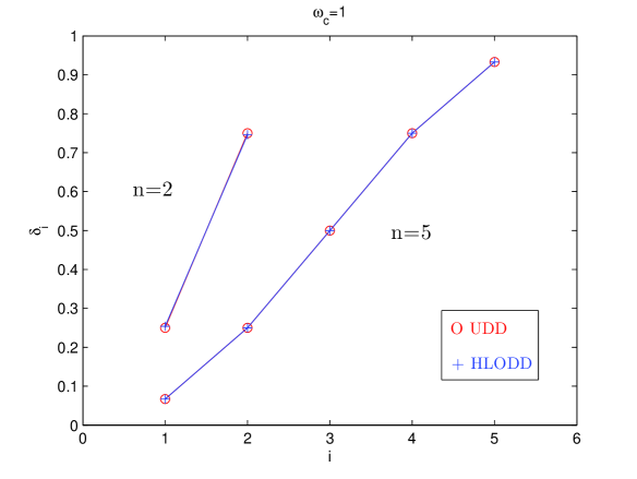
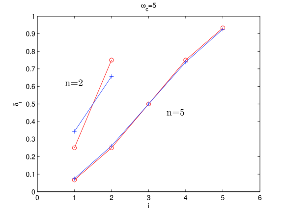
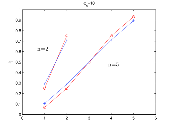
Figure 1: Comparison between UDD and HLODD sequence for different UV cutoff frequency $\omega_{c}$. Pulse sequences $\delta_{i}$ for $n=2$ and $n=5$ are plotted in one figure under the same $\omega_{c}$.

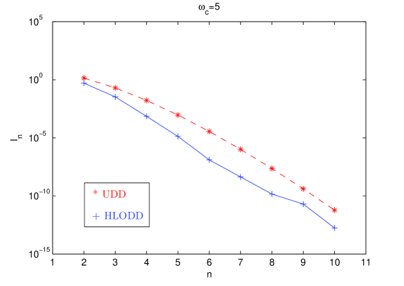
Figure 2: Semi-log plot of $I_{n}$ versus pulse number $n$. UDD and HLODD sequences are compared.

IV NUMERICAL RESULTS

We start our simulation by solving the non-linear equations ($13$) and evaluate the decoherence function with these solutions. First, we set the total evolution time $t=1$ without loss of generality. Then $z_{c}=\omega_{c}$ and we can concentrate on analyzing the influence of the cutoff frequency $\omega_{c}$. Computing solutions to ($13$) for different $\omega_{c}$, we find that the optimal pulse sequences behave differently. We also evaluate the UDD sequence for comparison.

As shown in Fig. 1, deviation of the pulse locations $\delta_{i}$ in HLODD sequence from their UDD counterparts increases with $\omega_{c}$. This agrees with our intuition since UDD focuses on suppressing decoherence by minimizing $|y_{n}(z)|$ in the neighborhood of $y_{n}(0)$, weakening its ability to maintain small $|y_{n}(z)|$ on the other end of the spectrum. For large $\omega_{c}$, UDD sequence is no longer optimal. In addition, we can see pulse number $n$ plays an important role. By increasing $n$, UDD can narrow the difference from HLODD. The difference between the two sequences when $n=2$ is greatly reduced when we increase $n$ to $5$, see Fig. 1. Especially for the case $\omega_{c}=1$, the difference is completely removed. However, for larger $\omega_{c}$ this gap can’t be removed by increasing $n$.

Next, to demonstrate the optimal decoupling ability of HLODD sequence, we compute $I_{n}$ versus $n$ while $\omega_{c}$ is chosen to be $5$. The results are depicted in Fig. 2, and again are compared with UDD. The obtained solutions yield a significant improvement over UDD. For fixed $n$, the HLODD suppresses decoherence better than UDD by one or two orders of magnitude which is in agreement with the results in Biercuk et al. (2009a); Uys et al. (2009), where LODD and OFDD sequences are tested for ⁹Be⁺ qubits in a penning ion trap and various spectrum. The qubit error rates are below $10^{-5}$ when $n>5$, and we see that HLODD is capable of suppressing the error rates far below the Fault-Tolerance error threshold Nielsen and Chuang (2000) by increasing $n$. Furthermore, by inspecting the points on the HLODD curve, we expect the HLODD sequence suppresses decoherence in power law $n$ as UDD.

At last, we would like to explain the numerical results in another way. If we fixed UV cutoff frequency $\omega_{c}$ at the beginning, and compare the HLODD performance for $t=1$, $t=5$, and $t=10$, the numerical results would be the same since $z_{c}$ did not change. So we can also conclude that for the same number of pulses $n$, HLODD will beat UDD with increasing total evolution time $t$.

V CONCLUSIONS

In this paper we analytically find the optimal pulse locations to decouple a qubit in an ohmic environment. By deriving the analytical expressions for the derivatives of decoherence function, we obtain a set of non-linear equations which the optimal pulse sequence must obey. These equations are completely different from UDD and are more accurate, because they incorporate the effect of UV cutoff frequency $\omega_{c}$.

In our numerical simulation, the analytical results provide an improvement over UDD sequence by an order or two of magnitude, which is consistent with previous results in LODD and OFDD obtained by purely numerical minimization and experimental feedback. We have to mention that the pulse performance is influenced by the sharp UV cutoff frequency $\omega_{c}$ greatly. The larger the UV cutoff $\omega_{c}$, the more HLODD deviates from UDD. Early work Pasini and Uhrig (2009); Biercuk et al. (2009a); Cywinski et al. (2008); Uhrig (2008) has pointed out that for soft large UV cutoff, UDD performs even worse and LODD is still a better choice. However, the integral ($3$) for $S(\omega)$ with a soft cutoff is hard to analyze.

In conclusion, our work provides an analytical solution to optimal dynamical decoupling for ohmic case. Our derivation is based on ohmic spectrum, but we believe it can be extended to super-ohmic case $S(\omega)\sim\omega^{\alpha}(\alpha>1)$ via slight modification.