Nonlinear diffusion model for Rayleigh-Taylor mixing

Abstract

The complex evolution of turbulent mixing in Rayleigh-Taylor convection is studied in terms of eddy diffusiviy models for the mean temperature profile. It is found that a non-linear model, derived within the general framework of Prandtl mixing theory, reproduces accurately the evolution of turbulent profiles obtained from numerical simulations. Our model allows to give very precise predictions for the turbulent heat flux and for the Nusselt number in the ultimate state regime of thermal convection.

Turbulent thermal convection is one of the most important manifestations of turbulence. It appears in many natural phenomena, from heat transport in stars to atmosphere and oceanic mixing, and it also plays a fundamental role in many technological applications Siggia (1994).

This Letter is devoted to the study of turbulent convection in the Rayleigh-Taylor (RT) setup, a paradigmatic configuration in which a heavy layer of fluid is placed on the top of a light layer. Gravitational instability at the interface of the two layers leads to a turbulent mixing zone which grows in time at the expenses of available potential energy Sharp (1984). Specific applications of RT convection range from cloud formation Schultz and et al. (2006), to supernova explosion Zingale et al. (2005); Cabot and Cook (2006) and solar corona heating Isobe et al. (2005). Because of the absence of boundaries, the phenomenology of RT turbulence results simpler than other convective systems where the thermal forcing is provided by walls, such as the Rayleigh-Benard configuration.

Recent theoretical work Chertkov (2003), confirmed by numerical simulations Dalziel et al. (1999); Cabot and Cook (2006); Cabot (2006); Vladimirova and Chertkov (2009); Boffetta et al. (2009); Celani et al. (2006); Matsumoto (2009), predicts for RT turbulence at small scales a turbulent cascade with Kolmogorov-Obukhov scaling (Bolgiano scaling in two dimensions). Here we concentrate on large scale features of RT turbulence. We propose a simple closure scheme based on the general framework of Prandtl mixing length theory and leading to a nonlinear diffusion model for temperature concentration. Our closure reproduces with high accuracy the spatial-temporal evolution of the mean temperature profile and allows to derive a prediction for the scaling law of $Nu$ versus $Ra$ which fits perfectly data obtained from direct numerical simulations.

The equation of motion for the incompressible velocity field ${\bf v}$ (${\bf\nabla}\cdot{\bf v}=0$) and temperature field $T$ in the Boussinesq approximation is

$$\partial_{t}{\bf v}+{\bf v}\cdot{\bf\nabla}{\bf v}=-{\bf\nabla}p+\nu\nabla^{2}{\bf v}-\beta{\bf g}T$$ (1)

$$\partial_{t}T+{\bf v}\cdot{\bf\nabla}T=\kappa\nabla^{2}T$$ (2)

where $\beta$ is the thermal expansion coefficient, $\nu$ the kinematic viscosity, $\kappa$ the thermal diffusivity and ${\bf g}=(0,0,-g)$ is the gravitational acceleration.

The initial condition (at $t=0$) is a layer of cooler (heavier) fluid on the top of a hotter (lighter) layer at rest, i.e. ${\bf v}({\bf x},0)=0$ and $T({\bf x},0)=-(\theta_{0}/2)\mbox{sgn}(z)$ where $\theta_{0}$ is the initial temperature jump which fixes the Atwood number $A=(1/2)\beta\theta_{0}$ ($T=0$ is the reference mean temperature). This configuration is unstable and after the linear instability phase, the system develops a turbulent mixing zone which grows in time starting from the plane $z=0$. An example of the turbulent temperature field obtained from high resolution direct numerical simulations of (1-2) is shown in Fig. 1.

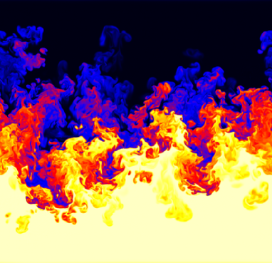
Figure 1: (color online). Snapshot of a $(x,z)$ section of the temperature field for Rayleigh-Taylor turbulence numerical simulation. White (black) represents hot, light (cold, heavy) fluid. Boussinesq equations (1-2) are integrated by a standard fully dealiased pseudo-spectral code at resolution $N_{x}\times N_{y}\times N_{z}$ with $N_{y}=N_{x}$ and aspect ratio $L_{x}/L_{z}=N_{x}/N_{z}=r$ (here $N_{x}=1024$ and $r=1$). Other parameters are $\beta g=0.5$, $\theta_{0}=1$ ($Ag=0.25$), $Pr=\nu/\kappa=1$ and $\nu$ is chosen such that $k_{\max}\eta\geq 1.2$ in all runs at final time. Initial perturbation is seeded by adding a $10\%$ of white noise to the initial temperature profile in a small layer around $z=0$.

In the mixing layer turbulent kinetic energy $E=(1/2)\langle v^{2}\rangle$ is produced at the expense of potential energy $P=-\beta g\langle zT\rangle$ as the energy balance indicates

$$-{dP\over dt}=\beta g\langle wT\rangle={dE\over dt}+\varepsilon_{\nu}$$ (3)

where $\varepsilon_{\nu}=\nu\langle(\partial_{\alpha}v_{\beta})^{2}\rangle$ is the viscous energy dissipation and $\langle\rangle$ represents the integral over the physical domain. Assuming that in the turbulent state all quantities in (3) scale in the same way one can balance $dv_{rms}^{2}/dt\simeq\beta g\theta_{0}v_{rms}$ (because temperature fluctuations are bounded by the initial jump $\theta_{0}$) and therefore one obtains the temporal scaling of velocity fluctuations $v_{rms}\simeq\beta g\theta_{0}t\simeq Agt$, i.e. a motion forced with constant acceleration $g$.

The accelerated growth of the width of the mixing layer is one of the standard diagnostics in the studies of RT turbulence Dalziel et al. (1999); Clark (2003); Huang et al. (2007); Kadau et al. (2007). Several definitions for the width have been proposed, based on either local or global properties of the mean temperature profile $\overline{T}(z,t)\equiv 1/(L_{x}L_{y})\int T({\bf x},t)dxdy$. The simplest measure $h_{r}$ is based on the threshold value of $z$ at which $\overline{T}(z,t)$ reaches a fraction $r$ of the maximum value i.e. $\overline{T}(\pm h_{r}(t)/2,t)=\mp r\theta_{0}/2$ Dalziel et al. (1999). This local definition of $h$ can be rather noisy and therefore alternative definitions based on integral quantities have been proposed Andrews and Spalding (1990); Dalziel et al. (1999); Cabot and Cook (2006)

$$h_{M}\equiv\int_{-L_{z}/2}^{L_{z}/2}M(\overline{c})dz$$ (4)

where $c=(T_{max}-T)/(T_{max}-T_{min})=1/2-T/\theta_{0}$ is the normalized dimensionless temperature ($0\leq c\leq 1$) and $M$ is a mixing function which has support on the mixing layer only, e.g. a logistic function $M(c)=4c(1-c)$ Vladimirova and Chertkov (2009) or a tent function $M(c)=2c+(2-4c)\theta(c-1/2)$ Cabot and Cook (2006). Dimensionally, $h$ is expected to grow with accelerated law $h(t)=\alpha Agt^{2}$ with the dimensionless coefficient $\alpha$ which depends on the definition of $h$ and apparently also on the form of the initial perturbation of the interface Dimonte and et al. (2004); Kadau et al. (2007). Recent studies Ristorcelli and Clark (2004); Cabot and Cook (2006) have shown that a more robust and consistent determination of $\alpha$ can be obtained if an initial time $t_{0}\neq 0$ is taken into account (physically representing the offset at which the $t^{2}$ law sets in) suggesting the possibility of a universal value, independent on the form of the initial perturbation.

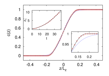
Figure 2: (color online). Normalized mean temperature profile $c(z)$ computed by averaging over horizontal planes the turbulent temperature field of Fig. 1. Blue dotted line is the prediction of the linear diffusion model (7). Black continuous line is the fit with the nonlinear model (10). Lower inset: enlargement of the temperature profile at the edge of the mixing layer. Upper inset: evolution of $z_{1}$ obtained by fitting the temperature profile with (10) at different times and over four different realizations. The line represents the fit $z_{1}=\gamma Ag(t+t_{0})^{2}$ which gives $\gamma\simeq 0.025$ and $t_{0}\simeq 3.3$.

The evolution equation for the normalized temperature profile $\overline{c}(z,t)$ is obtained by averaging (2) over the horizontal directions (assumed periodic)

$$\partial_{t}\overline{c}+\partial_{z}\overline{wc}=\kappa\partial_{z}^{2}\overline{c}$$ (5)

where $w$ represent the vertical velocity. The thermal flux term $\overline{wc}$ makes (5) not closed. Following a common approach in turbulence, we close this equation in terms of an eddy diffusivity $K(z,t)$ so that (5) is rewritten as

$$\partial_{t}\overline{c}=\partial_{z}K(z,t)\partial_{z}\overline{c}$$ (6)

Molecular diffusivity $\kappa$, included additively in $K(z,t)$, can be neglected for large scale properties at high Péclet number. The simplest approximation is to consider $K$ independent on $z$. For our problem, being a diffusion coefficient (i.e. a velocity time a scale) the eddy diffusivity is expected to depend on $t$ as $K(t)=b^{2}(Ag)^{2}t^{3}$ with $b$ a free dimensionless parameter. The self-similar solution to (6) with a step initial condition $\overline{c}(z,0)=\theta(z)$ is

$$\overline{c}(z,t)={1\over 2}\left[1+\mbox{erf}\left({z\over bAgt^{2}}\right)\right]$$ (7)

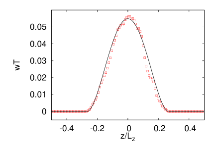
Figure 3: (color online). Heat flux profile $\overline{wT}$ obtained at the same time of Fig. 2. Black line represents the prediction of the nonlinear diffusion model as discussed in the text.

The constant diffusivity solution (7) is a relatively good approximation of the actual profile obtained from the numerical simulations of the full set of equations (1-2), as shown in Fig. 2. A closer inspection of the figure reveals that the model profile (7) is smoother than the actual profile at the edges of the mixing region (see inset of Fig. 2). The physical origin of this discrepancy is that turbulent mixing is not homogeneous within the mixing layer. Indeed turbulent velocity fluctuations decrease at the ends of the mixing region, and therefore a constant $K$ overestimates the diffusivity in these regions.

An improved model must therefore take into account a $z$-dependence of the diffusivity. Within the general framework of mixing length theory by Prandtl Prandtl (1925); Siggia (1994), the eddy diffusivity can be written as $K(z,t)\simeq H^{2}\partial_{z}V$ where $H$ represents a length characteristic of mixing and $V$ is the typical velocity fluctuation. Because velocity is driven by buoyancy at large scale, from equation (1) one can estimate that after a time $t$ the typical velocity is $V\propto\beta gTt$ and taking $H\propto h(t)$ one obtains for the eddy diffusivity $K(z,t)=a(Ag)^{3}t^{5}\partial_{z}\overline{c}$ where $a$ is again a dimensionless constant to be determined empirically. We remark that a similar approach, based on gradient dependent diffusivity, has been recently used for successfully modeling mixing in stratified flows Odier et al. (2009). Inserting the above expression in (6) one obtains a nonlinear diffusive model for the mean temperature profile

$$\partial_{t}\overline{c}=a(Ag)^{3}t^{5}\partial_{z}(\partial_{z}\overline{c})^{2}$$ (8)

Observe that the non-linearity of (8) reflects the fact that temperature fluctuations are not passive in this problem as they drive velocity fluctuations in (1).

Introducing the concentration derivative $\varphi(z,t)=3/(a(Ag)^{3})\partial_{z}\overline{c}(z,t)$ and a new time variable $t^{\prime}=t^{6}$, (8) is rewritten in a more standard form

$$\partial_{t^{\prime}}\varphi=\partial_{z}(\varphi^{n}\partial_{z}\varphi)$$ (9)

with $n=1$. Equation (9) represents a class of nonlinear diffusion equations with concentration dependent diffusivity well studied in different fields such as thermal waves in plasma radiation Zel’Dovich and Raizer (1969) and diffusion problems in porous media where for our case $n=1$ equation (9) is also known with the name of Boussinesq equation Bear (1988). The value of $n$ governs the behavior of the gradient when $\varphi\to 0$ which is finite for the present case. The self-similar solution (for general $n$ and dimensionality) is known Pattle (1959) and gives for our case

$$\begin{array}[]{lr}\overline{c}(z,t)={1\over 4}{z\over z_{1}}\left[3-\left({z\over z_{1}}\right)^{2}\right]+{1\over 2}&\qquad|z|\leq z_{1}\\ \overline{c}(z,t)=0&z<-z_{1}\\ \overline{c}(z,t)=1&z>z_{1}\end{array}$$ (10)

where $z_{1}(t)=\gamma Agt^{2}$ with $\gamma=(3a/2)^{1/3}$.

Having the analytical expression (10) for the mean concentration, the different definitions of the width of the mixing layer are all expressed in terms of $z_{1}$ and differ by a factor only (e.g. $h_{1}=2z_{1}$ and $h_{M}=(3/4)z_{1}$ for the tent function Cabot and Cook (2006)). Figure 2 shows that the polynomial function (10) fits very well the mean concentration profile obtained from numerical simulations. Runs at different resolutions (and viscosity, the only parameter in (1-2) when $Pr=1$) give analogous results. By fitting the numerical profiles at different times, one obtains the evolution of $z_{1}$ displayed in the inset of Fig. 2 which is consistent with the quadratic law $z_{1}=\gamma Ag(t+t_{0})^{2}$ ($t_{0}$ is the reference time as discussed above). The value obtained in this way for the coefficient is $\gamma=0.025\pm 0.002$ which for the profile $h_{M}$ gives $\alpha=(3/4)\gamma\simeq 0.019$ in agreement with previous numerical results Cabot and Cook (2006); Vladimirova and Chertkov (2009).

The nonlinear diffusion model can be extended from geometrical quantities to study the evolution of dynamical properties of turbulent convection. In particular, in the limit of small thermal diffusivity, from (5) and (8) one has an expression for the turbulent heat flux in terms of the mean temperature profile $\overline{wT}=a(Ag)^{3}t^{5}(\partial_{z}T)^{2}/\theta_{0}$. Figure 3 shows that the numerically measured profile of the heat flux is indeed quite close to the model prediction, a justification a posteriori of the proposed nonlinear closure scheme. Using the definition in (3) the loss of potential energy in kinetic energy (and dissipation) is written as $-dP/dt=(4/5)\gamma^{2}(Ag)^{3}t^{3}$ which shows that $\gamma$ is a measure of the efficiency of conversion of available potential energy in the turbulent flow.

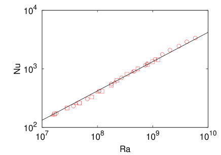
Figure 4: Nusselt number $Nu=\langle wT\rangle/(\kappa\theta_{0})$ versus Rayleigh number $Ra=Agh^{3}/(\nu\kappa)$ from three different set of simulations at resolutions $256\times 256\times 1024$ (squares), $512\times 512\times 2048$ (circles) and $1024\times 1024\times 1024$ (triangles) at $Pr=1$. Kinematic viscosities for the three runs are respectively $\nu=6\times 10^{-4}$, $\nu=3\times 10^{-4}$ and $\nu=1\times 10^{-4}$. The line is the prediction (11) with $\gamma=0.025$.

The relation between the heat flux and the profile geometry can be reformulated in terms of dimensionless quantities. Indeed, integrating over the width of the mixing layer it gives a relation between the Nusselt number $Nu=\langle wT\rangle/(\kappa\theta_{0})$ (the ratio of convective to conductive heat transfer) and the Rayleigh number $Ra=Agh^{3}/(\nu\kappa)$ (the ratio of the buoyancy forces to diffusivities). Using the expression (10) and for the length $h=h_{1}=2z_{1}$, one obtains the temporal evolution laws for the two quantities as $Ra=8\gamma^{3}(Ag)^{4}t^{6}/(\nu\kappa)$, $Nu=2\gamma^{2}(Ag)^{2}t^{3}/(5\kappa)$ and therefore the relation

$$Nu={1\over 5\sqrt{2}}\gamma^{1/2}Pr^{1/2}Ra^{1/2}$$ (11)

Equation (11) represents the well known Kraichnan’s prediction for the “ultimate state of thermal convection” Kraichnan (1962); Grossmann and Lohse (2000) which is a regime of turbulent convection expected to hold when the contribution of thermal and kinetic boundary layers becomes negligible. Because of the absence of boundaries, RT turbulence is a natural candidate for the appearance of this regime which has indeed been observed recently in numerical simulations both in two and three dimensions Lohse and Toschi (2003); Celani et al. (2006); Boffetta et al. (2009). Figure 4 shows that the prediction (11) with $\gamma=0.025$ fits well the numerical data obtained from a set of simulations at different resolutions. The fact that $Nu\gg 1$ is a posteriori confirmation of the negligible contribution of thermal diffusivity.

It is interesting to observe that the above result for $Nu$ satisfies a general bound which can be easily obtained starting from (5). Neglecting thermal diffusivity and assuming a self-similar evolution of the profile $\overline{c}(z,t)=f(z/z_{1}(t))$ with the symmetry condition $f(-z)=1-f(z)$, integrating (5) over the $z$ domain $[-L_{z}/2,L_{z}/2]$ twice, one obtains

$$\int_{-L_{z}\over 2}^{L_{z}\over 2}dz\overline{wc}={2\dot{z}_{1}\over z_{1}}\left[2\int_{0}^{L_{z}\over 2}dzz\overline{c}(z,t)-{L_{z}^{2}\over 4}\right]$$ (12)

Using the fact that for $z>0$ $\overline{c}(z,t)>1/2$ and assuming that the flow is still unmixed, $\overline{c}(z,t)=1$ for $z>z_{1}$, we get a bound

$$Nu=-{1\over\kappa}\int_{-L_{z}\over 2}^{L_{z}\over 2}dz\overline{wc}\leq{1\over\kappa}z_{1}\dot{z}_{1}$$ (13)

If we now further assume the accelerated growth of the mixing layer, $z_{1}(t)=\gamma Agt^{2}$ we end with a bound on the growth of the Nusselt number

$$Nu\leq{2\over\kappa}\gamma^{2}(Ag)^{2}t^{3}$$ (14)

which is indeed satisfied by our model. The physical interpretation of this bound is transparent: the growth of the heat flux follows the dimensional $t^{3}$ law with a coefficient which depends on the shape of the mean temperature profile. Maximum growth (14) is achieved when $c(z,t)=1/2$ for $-z_{1}\leq z\leq z_{1}$ which means a perfect mixing within the mixing layer. This would correspond to a coefficient $(\gamma/2)^{1/2}$ in (11).

In this Letter we have introduced a nonlinear diffusion model with a gradient dependent eddy diffusivity which reproduces accurately the large scale phenomenology of Rayleigh-Taylor turbulence obtained from high-resolution numerical simulations. The model contains a single free parameter, a measure of the turbulence production efficiency, which is directly related to the rate of accelerated growth of the mixing layer. The proposed closure scheme represents an important step for a phenomenological description of RT turbulence as it connects the evolution of the Nusselt number to the growth of the mixing layer, a global geometrical quantity which can be easily obtained in experiments.

References

- Siggia (1994) E. Siggia, Ann. Rev. Fluid Mech. 26, 137 (1994).
- Sharp (1984) D. H. Sharp, Physica D 12, 3 (1984).
- Schultz and et al. (2006) D. Schultz and et al., J. Atmos. Sci. 63, 2409 (2006).
- Zingale et al. (2005) M. Zingale, S. Woosley, C. Rendleman, M. Day, and J. Bell, Astrophys. J. 632, 1021 (2005).
- Cabot and Cook (2006) W. Cabot and A. Cook, Nature Physics 2, 562 (2006).
- Isobe et al. (2005) H. Isobe, T. Miyagoshi, K. Shibata, and T. Yokoyama, Nature 434, 478 (2005).
- Chertkov (2003) M. Chertkov, Phys. Rev. Lett. 91, 115001 (2003).
- Dalziel et al. (1999) S. Dalziel, P. Linden, and D. Youngs, J. Fluid Mech. 399, 1 (1999).
- Cabot (2006) W. Cabot, Phys. Fluids 18, 045101 (2006).
- Vladimirova and Chertkov (2009) N. Vladimirova and M. Chertkov, Physics of Fluids 21, 015102 (2009).
- Boffetta et al. (2009) G. Boffetta, A. Mazzino, S. Musacchio, and L. Vozella, Phys. Rev. E 79, 065301(R) (2009).
- Celani et al. (2006) A. Celani, A. Mazzino, and L. Vozella, Phys. Rev. Lett. 96, 134504 (2006).
- Matsumoto (2009) T. Matsumoto, Phys. Rev. E 79, 055301(R) (2009).
- Clark (2003) T. T. Clark, Phys. Fluids 15, 2413 (2003).
- Huang et al. (2007) Z. Huang, A. DeLuca, T. J. Atherton, M. Bird, C. Rosenblatt, and P. Carlès, Phys. Rev. Lett. 99, 204502 (2007).
- Kadau et al. (2007) K. Kadau, C. Rosenblatt, J. Barber, T. Germann, Z. Huang, P. Carles, and B. Alder, Proc. Nat. Acad. Sciences 104, 7741 (2007).
- Andrews and Spalding (1990) M. J. Andrews and D. B. Spalding, Phys. Fluids A 2, 922 (1990).
- Dimonte and et al. (2004) G. Dimonte and et al., Phys. Fluids 16, 1668 (2004).
- Ristorcelli and Clark (2004) J. Ristorcelli and T. Clark, J. Fluid Mech. 507, 213 (2004).
- Prandtl (1925) L. Prandtl, Z. Angew. Math. Mech 5, 136 (1925).
- Odier et al. (2009) P. Odier, J. Chen, M. K. Rivera, and R. E. Ecke, Phys. Rev. Lett. 102, 134504 (2009).
- Zel’Dovich and Raizer (1969) Y. Zel’Dovich and Y. Raizer, Ann. Rev. Fluid Mech. 1, 385 (1969).
- Bear (1988) J. Bear, Dynamics of fluids in porous media (Dover Publications, 1988).
- Pattle (1959) R. E. Pattle, Quart. Journ. Mech. and Applied Math. 12, 407 (1959).
- Kraichnan (1962) R. Kraichnan, Phys. Fluids 5, 1374 (1962).
- Grossmann and Lohse (2000) S. Grossmann and D. Lohse, J. Fluid Mech. 407, 27 (2000).
- Lohse and Toschi (2003) D. Lohse and F. Toschi, Phys. Rev. Lett. 90, 034502 (2003).