The inverse electromagnetic scattering problem in a piecewise homogeneous medium

Abstract

This paper is concerned with the problem of scattering of time-harmonic electromagnetic waves from an impenetrable obstacle in a piecewise homogeneous medium. The well-posedness of the direct problem is established, employing the integral equation method. Inspired by a novel idea developed by Hähner [11], we prove that the penetrable interface between layers can be uniquely determined from a knowledge of the electric far field pattern for incident plane waves. Then, using the idea developed by Liu & Zhang [22], a new mixed reciprocity relation is obtained and used to show that the impenetrable obstacle with its physical property can also be recovered. Note that the wave numbers in the corresponding medium may be different and therefore this work can be considered as a generalization of the uniqueness result of [20].

1 Introduction

We consider the scattering of time-harmonic electromagnetic plane waves with frequency $\omega>0$ by an impenetrable obstacle which is embedded in a piecewise homogeneous medium. For simplicity, and without loss of generality, in this paper we restrict ourself to the case where the obstacle is buried in a two-layered piecewise homogeneous medium, as shown in Figure 1. Note that our method and results can be easily extended to the multi-layered case. Precisely, let $\Omega_{2}\subset{\mathbb{R}}^{3}$ denote the impenetrable obstacle which is an open bounded region with a $C^{2}$ boundary $S_{1}$ and let ${\mathbb{R}}^{3}\backslash\overline{\Omega_{2}}$ denote the the background medium which is divided by means of a closed $C^{2,\alpha}\;(0<\alpha<1)$ surface $S_{0}$ into two connected domains $\Omega_{0}$ and $\Omega_{1}$. Let $\Omega$ denote the complement of $\Omega_{0}$, that is, $\Omega:={\mathbb{R}}^{3}\backslash\overline{\Omega_{0}}$. We assume that the boundary $S_{1}$ of the obstacle $\Omega_{2}$ has a dissection $S_{1}=\overline{\Gamma}_{1}\cup\overline{\Gamma}_{2}$, where $\Gamma_{1}$ and $\Gamma_{2}$ are two disjoint, relatively open subsets of $S_{1}$.

The electromagnetic properties of the homogeneous medium in $\Omega_{0}$ are described by space independent electric permittivity $\epsilon_{0}>0$, magnetic permeability $\mu_{0}>0$ and vanishing electric conductivity $\sigma_{0}=0$. The electromagnetic properties of the homogeneous medium in $\Omega_{1}$ are determined by space independent electric permittivity $\epsilon_{1}>0$, magnetic permeability $\mu_{1}>0$ and electric conductivity $\sigma_{1}\geq 0$. We define the wave number $k_{j}$ in the corresponding medium $\Omega_{j}$ by $k_{j}^{2}=(\epsilon_{j}+i\sigma_{j}/\omega)\mu_{j}\omega^{2}$ with $\Re k_{j}>0,\Im k_{j}\geq 0\;(j=0,1)$.

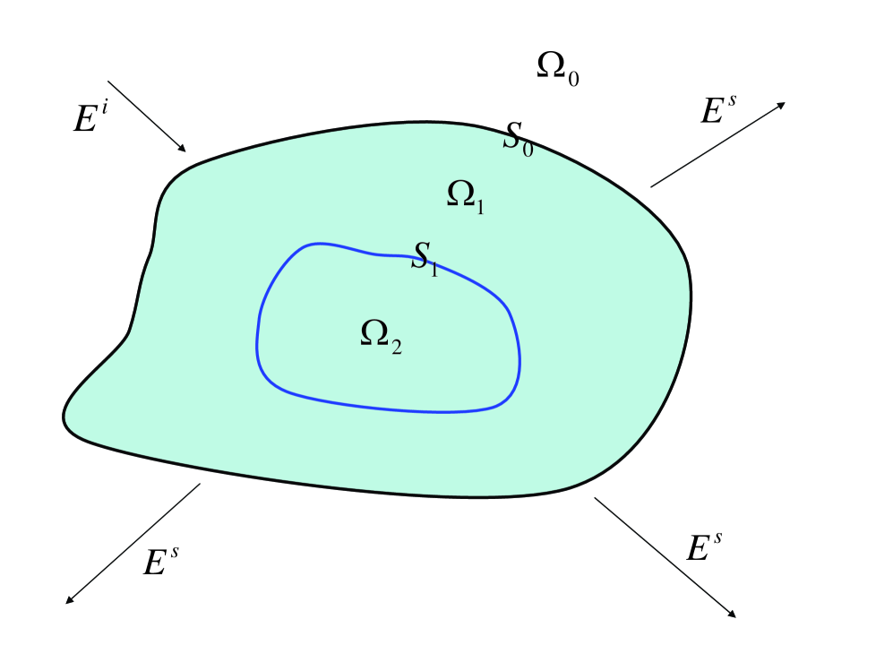
Fig. 1: Scattering in a two-layered background medium

For convenience we denote by $T(S_{j})$ and $T^{0,\alpha}(S_{j})\;(j=0,1)$, $0<\alpha<1$, the spaces of all continuous and uniformly Hölder continuous tangential fields equipped with the supremum norm and the Hölder norm, respectively. Then we introduce the normed spaces of tangential fields possessing a surface divergence (see section 6.3 in [8]) by

$$T_{d}(S_{j}) := \{a\in T(S_{j}):{\rm Div\,}a\in C(S_{j})\},$$

$$T_{d}^{0,\alpha}(S_{j}) := \{a\in T^{0,\alpha}(S_{j}):{\rm Div\,}a\in C^{0,\alpha}(S_{j})\}.$$

Let $T^{2}(S_{j})$ denote the completion of $T(S_{j})$ with respect to the usual $L^{2}-$norm and $T_{d}^{2}(S_{j})$ denote the tangential fields in $T^{2}(S_{j})$ with a surface divergence in $L^{2}(S_{j})\;(j=0,1)$. We denote by $\nu(x)$ the unit normal vector to a surface at the point $x$. For a closed surface it is directed into the exterior of the surface. For two vectors $a,b\in{\mathbb{C}}^{3}$ we write $a\cdot b$ for the scalar product and $a\times b$ for the vector product.

Given four tangential fields $T_{1},T_{2}\in T_{d}^{0,\alpha}(S_{0}),T_{3}\in T_{d}^{0,\alpha}(\Gamma_{1})$ and $T_{4}\in T^{0,\alpha}(\Gamma_{2})$, the direct problem consists in finding a solution $E,H\in C^{1}(\Omega_{0})\cap C(\overline{\Omega_{0}}),\;F,G\in C^{1}(\Omega_{1})\cap C(\overline{\Omega_{1}})$ to the Maxwell equations

$${\rm curl\,}E-ik_{0}H=0,\qquad{\rm curl\,}H+ik_{0}E=0\qquad\mbox{in}\;\;\Omega_{0},$$ (1.1)

$${\rm curl\,}F-ik_{1}G=0,\qquad{\rm curl\,}G+ik_{1}F=0\qquad\mbox{in}\;\;\Omega_{1},$$ (1.2)

which satisfies the Silver-Müller radiation condition

$$\lim_{r\rightarrow\infty}(H\times x-rE)=0$$ (1.3)

where $r=|x|$ and the limit holds uniformly in all directions $x/r$, the transmission boundary conditions

$$\nu\times E-\lambda_{E}\nu\times F=T_{1},\qquad\nu\times H-\lambda_{H}\nu\times G=T_{2}\qquad\mbox{on}\;\;S_{0}$$ (1.4)

with constants $\lambda_{E}$ and $\lambda_{H}$ given by $\lambda_{E}=\sqrt{\epsilon_{0}/(\epsilon_{1}+i\sigma_{1}/\omega)}$, $\lambda_{H}=\sqrt{\mu_{0}/\mu_{1}}$, and the boundary condition

$$\mathscr{B}(F)=0\qquad\mbox{on}\;S_{1}$$

with the operator $\mathscr{B}$ depending on the nature of the obstacle $\Omega_{2}$. Precisely, the boundary condition on $S_{1}$ is understood as:

$$\nu\times F=T_{3}\qquad \mbox{on}\;\Gamma_{1},$$ (1.5)

$$\nu\times G-\frac{\lambda}{k_{1}}(\nu\times F)\times\nu=T_{4}\qquad \mbox{on}\;\Gamma_{2}.$$ (1.6)

with a positive constant $\lambda$. Note that the case $\Gamma_{2}=\emptyset$ corresponds to a perfectly conducting obstacle and the case $\Gamma_{1}=\emptyset$ leads to an impedance boundary condition corresponding to an obstacle which is not perfectly conducting but does not allow the electromagnetic wave to penetrate deeply into the obstacle. The scattering problems with mixed boundary conditions widely occur in practical applications, e.g., in the use of electromagnetic waves to detect ”hostile” objects where the boundary, or more generally a portion of the boundary, is coated with an unknown material in order to avoid detection. We refer to [3, 5, 6] for the physical relevance and practical implication of the electromagnetic scattering by obstacles with a mixed boundary condition in a homogeneous medium.

In the next section, an integral equation method is employed to establish the well-posedness of the direct problem. A mixed reciprocity relation will also be proved. These results will play an important role in the proof of the uniqueness results in the inverse problem.

The radiation condition (1.3) ensures uniqueness of solutions to the exterior boundary value problem and leads to an asymptotic behavior of the form

$$E(x)=\frac{e^{ik_{0}|x|}}{|x|}\left\{E^{\infty}(\widehat{x})+O(\frac{1}{|x|})\right\},\qquad\mbox{as}\;\;|x|\rightarrow\infty$$ (1.7)

uniformly in all directions $\widehat{x}={x}/{|x|}$, where the vector field $E^{\infty}$ defined on the unit sphere $S^{2}$ is known as the electric far field pattern.

We consider the scattering of electromagnetic plane waves

$$E^{i}(x,d,q) = \frac{i}{k_{0}}{\rm curl\,}{\rm curl\,}qe^{ik_{0}x\cdot d}=ik_{0}(d\times q)\times de^{ik_{0}x\cdot d},$$

$$H^{i}(x,d,q) = {\rm curl\,}qe^{ik_{0}x\cdot d}=ik_{0}d\times qe^{ik_{0}x\cdot d}$$

where the unit vector $d$ describes the direction of propagation and the constant vector $q$ gives the polarization. Then we have $T_{1}=-\nu\times E^{i}(x,d,q),T_{2}=-\nu\times H^{i}(x,d,q)$ on $S_{0}$, $T_{3}=0$ on $\Gamma_{1}$ and $T_{4}=0$ on $\Gamma_{2}$ in the boundary problem (1.1)-(1.6). Throughout this paper, we will indicate the dependence of the corresponding scattered field, total field and far field pattern on the incident direction $d$ and the polarization $q$ by writing $E^{s}(\cdot,d,q),H^{s}(\cdot,d,q)$, $E(\cdot,d,q),H(\cdot,d,q)$ and $E^{\infty}(\cdot,d,q),H^{\infty}(\cdot,d,q)$, respectively.

The inverse problem we consider in this paper is, given the wave numbers $k_{j}\;(j=0,1)$, the constants $\lambda_{E}$ and $\lambda_{H}$ and the electric far field pattern $E^{\infty}(\widehat{x},d,q)$ for all observation directions $\widehat{x}\in S^{2}$, all incident directions $d\in S^{2}$ and all polarizations $q\in{\mathbb{R}}^{3}$, to determine the interface $S_{0}$ and the obstacle $\Omega_{2}$ with its physical property $\mathscr{B}$. As usual in most of the inverse problems, the first question to ask in this context is the identifiability, i.e. whether an obstacle can be identified from knowledge of its far-field pattern. Mathematically, the identifiability is the uniqueness issue which is of theoretical interest and is required in order to proceed to efficient numerical methods of solutions.

For scattering problems in a homogeneous medium, there has been an extensive study in the literature; see, e.g., uniqueness results for scattering from a perfect conductor by Colton & Kress [8], for scattering from an impenetrable obstacle with the boundary condition (1.6) by Kress [17], for scattering from a penetrable obstacle with transmission boundary conditions by Hähner [11] and for scattering from a penetrable obstacle with conductivity boundary conditions by Hettlich [9]. However, few results are available for the case of a piecewise homogeneous background medium. For the scalar Helmholtz equation, uniqueness results have been investigated in our recent paper [21]. Motivated by Isakov’s paper [12], Kirsch & Kress [14] gave another proof of the unique determination of a penetrable obstacle in a homogeneous medium for the scalar transmission problem. Based on their ideas, Hähner proved the unique determination of the penetrable obstacle in the electromagnetic scattering using a novel method. In this paper, we will use Hähner’s method to prove that the interface $S_{0}$ is uniquely determined from the electric far field patterns in Section 3. Under the condition that the wave numbers in the innermost and outermost homogeneous layers coincide, that is, $k_{0}=k_{1}$ in the Maxwell equations (1.1)-(1.2) and $S_{0}$ is known in advance, we have proved in [20] that the obstacle with its physical property can be uniquely determined. A main tool used and established in [20] is a mixed reciprocity relation which is important in the proof of the uniqueness result. In this paper, we establish a modified mixed reciprocity relation (cf. Lemma 2.5 in [22] for the acoustic scattering). Based on this result, we will prove the unique determination of the obstacle $\Omega_{2}$ and its physical property $\mathscr{B}$ in Section 4.

2 The direct scattering problem

We first show that the direct scattering problem has a unique solution.

Theorem 1.

The boundary value problem $(\ref{0EH})-(\ref{0ibc})$ admits at most one solution.

Proof.

Clearly, it is enough to show that $E=H=0$ in $\Omega_{0}$, $F=G=0$ in $\Omega_{1}$ for the corresponding homogeneous problem, that is, $T_{1}=T_{2}=0$ on $S_{0}$, $T_{3}=0$ on $\Gamma_{1}$ and $T_{4}=0$ on $\Gamma_{2}$. Using Green’s vector theorem, we have

$$\int_{S_{0}}\nu\times E\cdot\overline{H}ds = \int_{S_{0}}\nu\times E\cdot[(\nu\times\overline{H})\times\nu]ds$$ (2.1)

$$= \lambda_{E}\lambda_{H}\int_{S_{0}}\nu\times F\cdot[(\nu\times\overline{G})\times\nu]ds$$ (2.2)

$$= \lambda_{E}\lambda_{H}\int_{S_{0}}\nu\times F\cdot\overline{G}ds$$ (2.3)

$$= \lambda_{E}\lambda_{H}\int_{S_{1}}\nu\times F\cdot\overline{G}ds+\lambda_{E}\lambda_{H}\int_{\Omega_{1}}({\rm curl\,}F\cdot\overline{G}-F\cdot{\rm curl\,}\overline{G})dx$$ (2.4)

$$= -\frac{\lambda_{E}\lambda_{H}}{\overline{k_{1}}}\int_{\Gamma_{2}}\lambda|\nu\times F|^{2}ds+i\lambda_{E}\lambda_{H}\int_{\Omega_{1}}(k_{1}|G|^{2}-\overline{k_{1}}|F|^{2})dx$$ (2.5)

where we have used the transmission boundary conditions (1.4) in the second equality, the Maxwell equations (1.1)-(1.2) and the boundary conditions (1.5)-(1.6) in the fifth equality. Taking the real part of (2.1), we have, on noting that $\lambda_{E}\lambda_{H}=k_{0}/k_{1}$, $\Re k_{1}>0$, $\Im k_{1}\geq 0$ and $\lambda>0$ that

$$\Re\int_{S_{0}}\nu\times E\cdot\overline{H}ds=-\frac{k_{0}}{|k_{1}|^{2}}\int_{\Gamma_{2}}\lambda|\nu\times F|^{2}ds-\frac{2k_{0}\Re k_{1}\Im k_{1}}{|k_{1}|^{2}}\int_{\Omega_{1}}|F|^{2}ds\leq 0.$$

Therefore, by Rellich’s lemma [8], it follows that $E=H=0$ in $\Omega_{0}$. The transmission boundary conditions (1.4) and Holmgren’s uniqueness theorem [15] imply that $F=G=0$ in $\Omega_{1}$, which completes the proof. ∎

Denote by $\Phi_{j}$ the fundamental solution of the Helmholtz equation with wave number $k_{j}\;(j=0,1)$, which is given by

$$\Phi_{j}(x,y)=\frac{e^{ik_{j}|x-y|}}{4\pi|x-y|},\qquad\ x,y\in{\mathbb{R}}^{3},x\neq y.$$ (2.6)

For convenience, let $\Gamma_{0}$ denote the interface $S_{0}$. Given two integrable vector fields $a$ on $S_{0}$ and $b$ on $\Gamma_{j}$ and an integral function $\psi$ on $\Gamma_{j},\;(j=1,2)$, we introduce the integral operators $M_{i,j}$ and $N_{i,j}$ , respectively, by

$$(M_{i,j}a)(x)=2\int_{S_{0}}\nu(x)\times{\rm curl\,}_{x}\{a(y)\Phi_{j}(x,y)\}ds(y),\qquad x\in\;\Gamma_{i}$$

$$(N_{i,j}a)(x)=2\nu(x)\times{\rm curl\,}{\rm curl\,}\int_{S_{0}}\nu(y)\times a(y)\Phi_{j}(x,y)ds(y),\qquad x\in\;\Gamma_{i}$$

for $i=0,1,2;j=0,1$, the operators $\widetilde{M}_{i,j}$ and $\widetilde{N}_{i,j}$, respectively, by

$$(\widetilde{M}_{i,j}b)(x)=2\int_{\Gamma_{j}}\nu(x)\times{\rm curl\,}_{x}\{b(y)\Phi_{1}(x,y)\}ds(y),\qquad x\in\;\Gamma_{i}$$

$$(\widetilde{N}_{i,j}b)(x)=2\nu(x)\times{\rm curl\,}{\rm curl\,}\int_{\Gamma_{j}}\nu(y)\times b(y)\Phi_{1}(x,y)ds(y),\qquad x\in\;\Gamma_{i}$$

for $i=0,1,2,j=1,2$ and the operators $\widetilde{S}_{i,j}$ and $\widetilde{K}_{i,j}$, respectively, by

$$(\widetilde{S}_{i,j}\psi)(x)=2\int_{\Gamma_{j}}\Phi_{1}(x,y)\psi(y)ds(y),\qquad x\in\;\Gamma_{i}$$

$$(\widetilde{K}_{i,j}\psi)(x)=2\int_{\Gamma_{j}}\frac{\partial\Phi_{1}(x,y)}{\partial\nu(y)}\psi(y)ds(y),\qquad x\in\;\Gamma_{i}$$

for $i=0,1,2,j=1,2$.

Theorem 2.

The boundary value problem $(\ref{0EH})-(\ref{0ibc})$ has a unique solution. The solution depends continuously on the boundary data in the sense that the operator mapping the given boundary data onto the solution is continuous from $T_{d}^{0,\alpha}(S_{0})\times T_{d}^{0,\alpha}(S_{0})\times T_{d}^{0,\alpha}(\Gamma_{1})\times T^{0,\alpha}(\Gamma_{2})$ into $C^{0,\alpha}(\overline{\Omega_{0}})\times C^{0,\alpha}(\overline{\Omega_{0}})\times C^{0,\alpha}(\overline{\Omega_{1}})\times C^{0,\alpha}(\overline{\Omega_{1}})$.

Proof.

The uniqueness of solutions follows from Theorem 1. We now prove the existence of solutions using the integral equation method. We seek a solution in the form

$$E(x) = \frac{\lambda_{H}k_{0}}{k_{1}}{\rm curl\,}\int_{S_{0}}a(y)\Phi_{0}(x,y)ds(y)+\lambda_{E}{\rm curlcurl\,}\int_{S_{0}}b(y)\Phi_{0}(x,y)ds(y),\qquad\qquad$$ (2.7)

$$H(x) = \frac{1}{ik_{0}}{\rm curl\,}E(x)$$ (2.8)

$$= \frac{\lambda_{H}}{ik_{1}}{\rm curlcurl\,}\int_{S_{0}}a(y)\Phi_{0}(x,y)ds(y)+\frac{\lambda_{E}k_{0}}{i}{\rm curl\,}\int_{S_{0}}b(y)\Phi_{0}(x,y)ds(y)\qquad\qquad$$ (2.9)

for $x\in\Omega_{0}$ and

$$F(x) = {\rm curl\,}\int_{S_{0}}a(y)\Phi_{1}(x,y)ds(y)+{\rm curlcurl\,}\int_{S_{0}}b(y)\Phi_{1}(x,y)ds(y)$$ (2.13)

$$+{\rm curl\,}\int_{\Gamma_{1}}c(y)\Phi_{1}(x,y)ds(y)+\frac{i}{k_{1}^{2}}{\rm curlcurl\,}\int_{\Gamma_{1}}\nu(y)\times(\widehat{S}_{1}^{2}c)(y)\Phi_{1}(x,y)ds(y)$$

$$+\int_{\Gamma_{2}}d(y)\Phi_{1}(x,y)ds(y)+i\lambda{\rm curl\,}\int_{\Gamma_{2}}\nu(y)\times(\widehat{S}_{2}^{2}d)(y)\Phi_{1}(x,y)ds(y)$$

$$+{\rm grad}\int_{\Gamma_{2}}\psi(y)\Phi_{1}(x,y)ds(y)+i\lambda\int_{\Gamma_{2}}\nu(y)\psi(y)\Phi_{1}(x,y)ds(y),$$

$$G(x) = \frac{1}{ik_{1}}{\rm curl\,}F(x)$$ (2.14)

$$= \frac{1}{ik_{1}}{\rm curlcurl\,}\int_{S_{0}}a(y)\Phi_{1}(x,y)ds(y)-ik_{1}{\rm curl\,}\int_{S_{0}}b(y)\Phi_{1}(x,y)ds(y)$$ (2.20)

$$+\frac{1}{ik_{1}}{\rm curlcurl\,}\int_{\Gamma_{1}}c(y)\Phi_{1}(x,y)ds(y)$$

$$+\frac{1}{k_{1}}{\rm curl\,}\int_{\Gamma_{1}}\nu(y)\times(\widehat{S}_{1}^{2}c)(y)\Phi_{1}(x,y)ds(y)$$

$$+\frac{1}{ik_{1}}{\rm curl\,}\int_{\Gamma_{2}}d(y)\Phi_{1}(x,y)ds(y)$$

$$+\frac{\lambda}{k_{1}}{\rm curlcurl\,}\int_{\Gamma_{2}}\nu(y)\times(\widehat{S}_{2}^{2}d)(y)\Phi_{1}(x,y)ds(y)$$

$$+\frac{\lambda}{k_{1}}{\rm curl\,}\int_{\Gamma_{2}}\nu(y)\psi(y)\Phi_{1}(x,y)ds(y)$$

for $x\in\Omega\setminus S_{1},$ where $a,b\in T_{d}^{0,\alpha}(S_{0}),c\in T_{d}^{0,\alpha}(\Gamma_{1}),d\in T^{0,\alpha}(\Gamma_{2})$ and $\psi\in C^{0,\alpha}(\Gamma_{2})$ are five densities to be determined and $\widetilde{S}_{j}$ is the single-layer operator given by

$$(\widehat{S}_{j}c)(x):=\frac{1}{2\pi}\int_{\Gamma_{j}}\frac{1}{|x-z|}c(z)ds(z),\qquad x\in\Gamma_{j},\;j=1,2.$$

If the densities $a,b\in T_{d}(S_{0}),c\in T_{d}^{0,\alpha}(\Gamma_{1}),d\in T^{0,\alpha}(\Gamma_{2})$ and $\psi\in C^{0,\alpha}(\Gamma_{2})$ satisfy the following system of integral equations (2.21)-(2.25), then we can conclude from the integral equations (2.21) and (2.22) that $a,b\in T_{d}^{0,\alpha}(S_{0})$. Therefore we choose the solution space $X:=T_{d}(S_{0})\times T_{d}(S_{0})\times T_{d}^{0,\alpha}(\Gamma_{1})\times T^{0,\alpha}(\Gamma_{2})\times C^{0,\alpha}(\Gamma_{2})$ for the system of integral equations (2.21)-(2.25) below. The vector field $F$ given by (2.13) clearly satisfies the vector Helmholtz equation and its cartesian components satisfy the Sommerfeld radiation condition. Hence, if we insist that ${\rm div}F=0$ in ${\mathbb{R}}^{3}\setminus\Gamma_{2}$, then by Theorems 6.4 and 6.7 in [8] we have that $F,G$ satisfy the Maxwell equations (1.2). Since ${\rm div}F$ satisfies the scalar Helmholtz equation and the Sommerfeld radiation condition, by the uniqueness for the exterior Dirichlet problem (see Theorem 3.7 in [8]) it suffices to impose ${\rm div}F=0$ only on the boundary $\Gamma_{2}$. Then the jump relations together with the regularity results of surface potentials imply that $E,H,F,G$ defined in (2.7)-(2.14) solve the direct problem provided the densities $a,b,c,d,\psi$ solve

$$\left(\lambda_{E}+\frac{\lambda_{H}k_{0}}{k_{1}}\right)a+L_{1}a+M_{1}b+N_{1}c+P_{1}d+Q_{1}\psi = 2T_{1}\quad{\rm on}\;S_{0},$$ (2.21)

$$\frac{\lambda_{E}k_{0}+\lambda_{H}k_{1}}{i}b+L_{2}a+M_{2}b+N_{2}c+P_{2}d+Q_{2}\psi = 2T_{2}\quad{\rm on}\;S_{0},$$ (2.22)

$$c+L_{3}a+M_{3}b+N_{3}c+P_{3}d+Q_{3}\psi = 2T_{3}\quad{\rm on}\;\;\Gamma_{1},$$ (2.23)

$$d+L_{4}a+M_{4}b+N_{4}c+P_{4}d+Q_{4}\psi = 2T_{4}\quad{\rm on}\;\;\Gamma_{2},$$ (2.24)

$$i\lambda\psi+P_{5}d+Q_{5}\psi = 0\qquad{\rm on}\;\;\Gamma_{2}$$ (2.25)

where

$$L_{1} := \frac{\lambda_{H}k_{0}}{k_{1}}M_{0,0}-\lambda_{E}M_{0,1},\hskip 71.13188ptM_{1}:=\lambda_{E}(N_{0,0}-N_{0,1})R,$$

$$N_{1} := -\lambda_{E}(\widetilde{M}_{0,1}+\frac{i}{k_{1}^{2}}\widetilde{N}_{0,1}P\widehat{S}_{1}^{2}),\hskip 54.06006ptP_{1}:=\lambda_{E}R\widetilde{S}_{0,2}+i\lambda\lambda_{E}\widetilde{M}_{0,2}R\widehat{S}_{2}^{2},$$

$$Q_{1}\psi := -2\lambda_{E}\nu(x)\times{\rm grad}\int_{\Gamma_{2}}\Phi_{1}(x,y)\psi(y)ds(y)+i\lambda\lambda_{E}R\widetilde{S}_{0,2}(\nu\psi),$$

$$L_{2} := \frac{\lambda_{H}}{ik_{1}}(N_{0,0}-N_{0,1})R,\hskip 82.51282ptM_{2}:=\frac{\lambda_{E}k_{0}}{i}M_{0,0}-\frac{\lambda_{H}k_{1}}{i}M_{0,1},\;\;$$

$$N_{2} := -\frac{\lambda_{H}}{ik_{1}}\widetilde{N}_{0,1}R+\frac{\lambda_{H}}{k_{1}}\widetilde{M}_{0,1}R\widehat{S}_{1}^{2},\hskip 31.2982ptP_{2}:=\frac{i\lambda_{H}}{k_{1}}\widetilde{M}_{0,2}-\frac{\lambda\lambda_{H}}{k_{1}}\widetilde{N}_{0,2}P\widehat{S}_{2}^{2},$$

$$Q_{2}\psi := -2\frac{\lambda\lambda_{H}}{k_{1}}\nu(x)\times{\rm curl\,}\int_{\Gamma_{2}}\nu(y)\psi(y)\Phi_{1}(x,y)ds(y),$$

$$L_{3} := M_{1,1},\qquad\qquad M_{3}:=N_{1,1}R,\hskip 42.67912ptN_{3}:=\widetilde{M}_{1,1}+\frac{i}{k_{1}^{2}}\widetilde{N}_{1,1}P\widehat{S}_{1}^{2},$$

$$P_{3} := -R\widetilde{S}_{1,2}-i\lambda\widetilde{M}_{1,2}R\widehat{S}_{2}^{2},$$

$$Q_{3}\psi: = 2\nu(x)\times{\rm grad}\int_{\Gamma_{2}}\Phi_{1}(x,y)\psi(y)ds(y)-i\lambda R\widetilde{S}_{1,2}(\nu\psi),$$

$$L_{4} := N_{2,1}-i\lambda RM_{2,1},\hskip 99.58464ptM_{4}:=k_{1}^{2}M_{2,1}-i\lambda RN_{2,1}R,$$

$$N_{4} := \widetilde{N}_{2,1}R-i\widetilde{M}_{2,1}R\widehat{S}_{1}^{2}-i\lambda R\widetilde{M}_{2,1}+\frac{\lambda}{k_{1}^{2}}R\widetilde{N}_{2,1}P\widehat{S}_{1}^{2},$$

$$P_{4} := \widetilde{M}_{2,2}+i\lambda\widetilde{N}_{2,2}P\widehat{S}_{2}^{2}-i\lambda P\widetilde{S}_{2,2}-\lambda^{2}R\widetilde{M}_{2,2}R\widehat{S}_{2}^{2}+\lambda^{2}P\widehat{S}_{2}^{2},$$

$$Q_{4}\psi := 2i\lambda\nu(x)\times\int_{\Gamma_{2}}{\rm grad}_{x}\Phi_{1}(x,y)\times\{\nu(y)-\nu(x)\}\psi(y)ds(y)+\lambda^{2}P\widetilde{S}_{2,2}(\nu\psi),$$

$$P_{5}d := -2\int_{\Gamma_{2}}{\rm grad}_{x}\Phi_{1}(x,y)\cdot d(y)ds(y),\hskip 28.45274ptQ_{5}=k_{1}^{2}\widetilde{S}_{2,2}+i\lambda\widetilde{K}_{2,2}.$$

Here $R,P$ are defined by $Ra:=a\times\nu$ and $Pa:=(\nu\times a)\times\nu,$ respectively.

Writing the system of integral equations (2.21)-(2.25) in the matrix form

$$\left(\begin{matrix}\lambda_{a}&0&0&0&0\\ 0&\lambda_{b}&0&0&0\\ 0&0&1&0&0\\ 0&0&0&1&0\\ 0&0&0&P_{5}&i\lambda\end{matrix}\right)\left(\begin{matrix}a\\ b\\ c\\ d\\ \psi\end{matrix}\right)+\left(\begin{matrix}L_{1}&M_{1}&N_{1}&P_{1}&Q_{1}\\ L_{2}&M_{2}&N_{2}&P_{2}&Q_{2}\\ L_{3}&M_{3}&N_{3}&P_{3}&Q_{3}\\ L_{4}&M_{4}&N_{4}&P_{4}&Q_{4}\\ 0&0&0&0&Q_{5}\end{matrix}\right)\left(\begin{matrix}a\\ b\\ c\\ d\\ \psi\end{matrix}\right)=\left(\begin{matrix}2T_{1}\\ 2T_{2}\\ 2T_{3}\\ 2T_{4}\\ 0\end{matrix}\right),$$

where $\lambda_{a}=\lambda_{E}+(\lambda_{H}k_{0})/k_{1}$ and $\lambda_{b}=-i\lambda_{E}k_{0}-i\lambda_{H}k_{1}$, we can see that the first matrix operator has a bounded inverse because of its triangular form and the second one is compact by Theorems 6.15 and 6.16 in [8] and the argument in the proof of Theorems 6.19 and 9.12 in [8]. Therefore the Riesz-Fredholm theory can be applied to prove the existence of a unique solution to the system (2.21)-(2.25) in the solution space $X$. To do this, let $a,b,c,d$ and $\psi$ be a solution to the homogeneous form of (2.21)-(2.25) (i.e., $T_{1}=T_{2}=0$ on $S_{0}$, $T_{3}=0$ on $\Gamma_{1}$ and $T_{4}=0$ on $\Gamma_{2}$). We then need to show that $a=b=c=d=\psi=0$. First, by Theorem 1 we conclude that $E=H=0$ in $\Omega_{0}$ and $F=G=0$ in $\Omega_{1}$.

Now, by the jump relations we have

$$-\nu\times F_{-}=c,\quad-\nu\times G_{-}=\frac{1}{k_{1}}\nu\times\widehat{S}_{1}^{2}c\qquad{\rm on}\;\;\Gamma_{1},$$ (2.26)

$$-\nu\times F_{-}=i\lambda\nu\times\widehat{S}_{2}^{2}d,\quad-\nu\times G_{-}=\frac{1}{ik_{1}}d\qquad{\rm on}\;\;\Gamma_{2},$$ (2.27)

$$-{\rm div}F_{-}=-i\lambda\psi,\quad-\nu\cdot F_{-}=-\psi\qquad{\rm on}\;\;\Gamma_{2}\;$$ (2.28)

where $F_{-},\;G_{-}$ denote the limit of $F,\;G$ on the surface $S_{1}$ from the interior of $S_{1}$, respectively. Hence, using Green’s vector theorem, we derive from (2.26)-(2.28) that

$$i\int_{\Gamma_{1}}|\widehat{S}_{1}c|^{2}ds+i\lambda\int_{\Gamma_{2}}|\widehat{S}_{2}d|^{2}ds+i\lambda\int_{\Gamma_{2}}|\psi|^{2}ds$$

$$= \int_{S_{1}}\{\nu\times\overline{F_{-}}\cdot{\rm curl\,}F+\nu\cdot\overline{F_{-}}{\rm div}F\}ds$$

$$= \int_{\Omega_{2}}\{|{\rm curl\,}F|^{2}+|{\rm div}F|^{2}-[(\Re k_{1})^{2}-(\Im k_{1})^{2}]|F|^{2}-2i\Re k_{1}\Im k_{1}|F|^{2}\}dx.$$

Taking the imaginary part of the last equation gives that $\psi=0$ on $\Gamma_{2}$, $\widehat{S}_{1}c=0$ on $\Gamma_{1}$ and $\widehat{S}_{2}d=0$ on $\Gamma_{2}$. This implies that $c=0$ on $\Gamma_{1}$, $d=0$ on $\Gamma_{2}$ (see the proof of Theorem 3.10 in [8]).

On the other hand, define

$$\widetilde{E}(x) = -m{\rm curl\,}\int_{S_{0}}a(y)\Phi_{0}(x,y)ds(y)-\frac{m\lambda_{E}k_{1}}{\lambda_{H}k_{0}}{\rm curlcurl\,}\int_{S_{0}}b(y)\Phi_{0}(x,y)ds(y),\;\;\qquad$$ (2.29)

$$\widetilde{H}(x) = \frac{1}{ik_{0}}{\rm curl\,}\widetilde{E}(x)$$ (2.30)

$$= \frac{im}{k_{0}}{\rm curlcurl\,}\int_{S_{0}}a(y)\Phi_{0}(x,y)ds(y)-\frac{m\lambda_{E}k_{1}}{i\lambda_{H}}{\rm curl\,}\int_{S_{0}}b(y)\Phi_{0}(x,y)ds(y)\qquad$$ (2.31)

for $x\in\Omega$ and

$$\widetilde{F}(x) = {\rm curl\,}\int_{S_{0}}a(y)\Phi_{0}(x,y)ds(y)+{\rm curlcurl\,}\int_{S_{0}}b(y)\Phi_{0}(x,y)ds(y),\;\;\qquad$$ (2.32)

$$\widetilde{G}(x) = \frac{1}{ik_{1}}{\rm curl\,}\widetilde{F}(x)$$ (2.33)

$$= \frac{1}{ik_{1}}{\rm curlcurl\,}\int_{S_{0}}a(y)\Phi_{0}(x,y)ds(y)-ik_{1}{\rm curl\,}\int_{S_{0}}b(y)\Phi_{0}(x,y)ds(y)\qquad$$ (2.34)

for $x\in\Omega_{0}$, where $m$ is a constant given by $m:=\sqrt{\lambda_{H}/\lambda_{E}}$. Then by the jump relations we have

$$\nu\times\widetilde{F}-\nu\times F=a,\qquad\frac{k_{1}}{\lambda_{H}k_{0}}\nu\times E+\frac{1}{m}\nu\times\widetilde{E}=a\qquad {\rm on}\;S_{0},\qquad$$ (2.35)

$$\nu\times\widetilde{G}-\nu\times G=-ik_{1}b,\qquad\frac{k_{1}}{\lambda_{E}k_{0}}\nu\times H+\frac{\lambda_{H}}{m\lambda_{E}}\nu\times\widetilde{H}=-ik_{1}b\qquad {\rm on}\;S_{0}.$$ (2.36)

Thus, $\widetilde{E},\widetilde{H},\widetilde{F},\widetilde{G}$ given by (2.29)-(2.33) solves the homogeneous transmission problem

$${\rm curl\,}\widetilde{F}-ik_{1}\widetilde{G}=0,\qquad{\rm curl\,}\widetilde{G}+ik_{1}\widetilde{F}=0\quad \mbox{in}\;\;\Omega_{0},$$ (2.37)

$${\rm curl\,}\widetilde{E}-ik_{0}\widetilde{H}=0,\qquad{\rm curl\,}\widetilde{H}+ik_{0}\widetilde{E}=0\quad \mbox{in}\;\;\Omega,$$ (2.38)

$$\nu\times\widetilde{F}-\frac{1}{m}\nu\times\widetilde{E}=0,\qquad\nu\times\widetilde{G}-\frac{\lambda_{H}}{m\lambda_{E}}\nu\times\widetilde{H}=0\quad \mbox{on}\;\;S_{0},$$ (2.39)

$$\lim_{|x|\rightarrow\infty}(\widetilde{H}\times x-|x|\widetilde{E})=0\quad$$ (2.40)

where the limit holds uniformly in all directions $x/|x|$. Similar to the argument as in the proof of Theorem 1, we find on using Green’s vector theorem and by the definition of $m$ that

$$\int_{S_{0}}\nu\times\widetilde{F}\cdot\overline{\widetilde{G}}ds = \int_{S_{0}}\nu\times\widetilde{F}\cdot[(\nu\times\overline{\widetilde{G}})\times\nu]ds=\int_{S_{0}}\nu\times\widetilde{E}\cdot[(\nu\times\overline{\widetilde{H}})\times\nu]ds$$

$$= \int_{\Omega}({\rm curl\,}\widetilde{E}\cdot\overline{\widetilde{H}}-\widetilde{E}\cdot{\rm curl\,}\overline{\widetilde{H}})dx=ik_{0}\int_{\Omega_{1}}(|\widetilde{H}|^{2}-|\widetilde{E}|^{2})dx$$

Taking the real part of the above equation, we have

$$\Re\int_{S_{0}}\nu\times\widetilde{F}\cdot\overline{\widetilde{G}}ds\leq 0.$$

Therefore, by Rellich’s lemma (see Theorem 4.17 in [7]), it follows that $\widetilde{F}=\widetilde{G}=0$ in $\Omega_{0}$. The transmission boundary conditions (2.39) and Holmgren’s uniqueness theorem [15] imply that $\widetilde{E}=\widetilde{H}=0$ in $\Omega$. Hence, by the relations (2.35) and (2.36), we conclude that $a=b=0$ on $S_{0}$, which completes the proof. ∎

As incident fields $E^{i}$, besides the electromagnetic plane waves we are also interested in the electromagnetic field of an electric dipole with polarization $p$ which is given by

$$E^{i}(x;z_{j},p)=\frac{i}{k_{j}}{\rm curlcurl\,}(p\Phi(x,z_{j})),\;\;\;H^{i}(x;z_{j},p)={\rm curl\,}(p\Phi_{j}(x,z_{j}))$$ (2.41)

located at the point $z_{j}\in\Omega_{j}$ for $x\neq z_{j}$ $(j=0,1)$. For $j=0,1$, denote by $E(\cdot;z_{j},p)$ and $H(\cdot;z_{j},p)$ the corresponding total waves, by $E^{s}(\cdot;z_{j},p)$ and $H^{s}(\cdot;z_{j},p)$ the scattered waves and by $E^{\infty}(\cdot;z_{j},p)$ and $H^{\infty}(\cdot;z_{j},p)$ the corresponding far field patterns, indicating the dependence on the location $z_{j}$ and polarization $p$ of the electric dipole.

Remark 3.

In the case when the incident field is given by the electric dipole $E^{i}(x;z_{0},p),H^{i}(x;z_{0},p)$ located at $z_{0}\in\Omega_{0}$, we have $E=E^{s}(x;z_{0},p),\;T_{1}=-\nu\times E^{i}(x;z_{0},p),\;T_{2}=-\nu\times H^{i}(x;z_{0},p),\;T_{3}=0$ and $T_{4}=0$ in the boundary value problem $(\ref{0EH})-(\ref{0ibc})$. In the case when the incident field is given by the electric dipole $E^{i}(x;z_{1},p),H^{i}(x;z_{1},p)$ located at $z_{1}\in\Omega_{1}$, we have $E=E(x;z_{1},p),\;T_{1}=\lambda_{E}\nu\times E^{i}(x;z_{1},p),\;T_{2}=\lambda_{H}\nu\times H^{i}(x;z_{1},p),\;T_{3}=-\nu\times E^{i}(x;z_{1},p)$ and $T_{4}=-\nu\times H^{i}(x;z_{1},p)+\frac{\lambda}{k_{1}}(\nu\times E^{i}(x;z_{1},p))\times\nu$ in the boundary value problem $(\ref{0EH})-(\ref{0ibc})$. Note that in the last case $E^{\infty}(\cdot;z_{1},p)$ is the electric far field pattern of the field $E(x;z_{1},p)=E^{s}(x;z_{1},p)$ for $x\in\Omega_{0}$. This is different from our early work [20], where the total field $E(x;z_{1},p)$ in $\Omega_{0}$ is decomposed into the scattered field $E^{s}(x;z_{1},p)$ and the incident field $E^{i}(x;z_{1},p)$, so $E^{\infty}(\cdot;z_{1},p)$ is the electric far field pattern of the scattered field $E^{s}(x;z_{1},p)$ rather than the total field $E(x;z_{1},p)$.

We now establish the following mixed reciprocity relation which is needed for the inverse problem.

Lemma 4.

(Mixed reciprocity relation) For scattering of plane waves $E^{i}(x,d,q)$ and electric dipole $E^{i}(x;z,p)$ from the obstacle $\Omega_{2}$ we have

$$4\pi q\cdot E^{\infty}(-d;z_{0},p)=p\cdot E^{s}(z_{0},d,q),\qquad z_{0}\in\Omega_{0},$$ (2.42)

$$4\pi q\cdot E^{\infty}(-d;z_{1},p)=\lambda_{E}\lambda_{H}p\cdot F(z_{1},d,q),\qquad z_{1}\in\Omega_{1}$$ (2.43)

for all incident directions $d\in S^{2}$ and all polarizations $p,q\in{\mathbb{R}}^{3}$.

Proof.

Arguing similarly as in the proof of Lemma 3.1 in [20], we have

$$4\pi q\cdot E^{\infty}(-d;z,p)$$ (2.44)

$$=\int_{S_{0}}\{\nu(y)\times E^{s}(y;z,p)\cdot H(y,d,q)+\nu(y)\times H^{s}(y;z,p)\cdot E(y,d,q)\}ds(y)$$ (2.45)

for all $z\in\Omega_{0}\cup\Omega_{1}$ and all $d\in S^{2},\;p,q\in{\mathbb{R}}^{3}$.

We first consider the case $z:=z_{0}\in\Omega_{0}$. Using a similar argument as in the proof of Lemma 3.1 in [20], we have

$$p\cdot E^{s}(z,d,q)$$ (2.46)

$$=\int_{S_{0}}\{\nu(y)\times H(y,d,q)\cdot E^{i}(y;z,p)-\nu(y)\times H^{i}(y;z,p)\cdot E(y,d,q)\}ds(y)$$ (2.47)

for all $z\in\Omega_{0}$ and all $d\in S^{2},\;p,q\in{\mathbb{R}}^{3}$. Subtract the equation (2.46) from the equation (2.44) to obtain that

$$4\pi q\cdot E^{\infty}(-d;z,p)-p\cdot E^{s}(z,d,q)$$

$$=\int_{S_{0}}\{\nu(y)\times E(y;z,p)\cdot H(y,d,q)+\nu(y)\times H(y;z,p)\cdot E(y,d,q)\}ds(y)$$

$$=\lambda_{E}\lambda_{H}\int_{S_{0}}\{\nu(y)\times F(y;z,p)\cdot G(y,d,q)+\nu(y)\times G(y;z,p)\cdot F(y,d,q)\}ds(y)$$

$$=\lambda_{E}\lambda_{H}\int_{S_{1}}\{\nu(y)\times F(y;z,p)\cdot G(y,d,q)+\nu(y)\times G(y;z,p)\cdot F(y,d,q)\}ds(y)$$

$$=0$$

for all $z\in\Omega_{0}$ and all $d\in S^{2},\;p,q\in{\mathbb{R}}^{3}$, where we have used the transmission boundary condition (1.4) in the second equality, Green’s vector theorem and Maxwell’s equations (1.2) in the third equality and the boundary conditions (1.5) and (1.6) in the fourth equality.

We now consider the case $z:=z_{1}\in\Omega_{1}$. Using the transmission boundary condition (1.4) and Green’s vector theorem, we deduce that

$$4\pi q\cdot E^{\infty}(-d;z,p)$$ (2.48)

$$= \lambda_{E}\lambda_{H}\int_{S_{0}}\{\nu(y)\times E^{i}(y;z,p)\cdot G(y,d,q)+\nu(y)\times H^{i}(y;z,p)\cdot F(y,d,q)\}ds(y)$$ (2.50)

$$+\lambda_{E}\lambda_{H}\int_{S_{0}}\{\nu(y)\times F(y;z,p)\cdot G(y,d,q)+\nu(y)\times G(y;z,p)\cdot F(y,d,q)\}ds(y)$$

$$= \lambda_{E}\lambda_{H}\int_{S_{0}}\{\nu(y)\times E^{i}(y;z,p)\cdot G(y,d,q)+\nu(y)\times H^{i}(y;z,p)\cdot F(y,d,q)\}ds(y)$$ (2.52)

$$+\lambda_{E}\lambda_{H}\int_{S_{1}}\{\nu(y)\times F(y;z,p)\cdot G(y,d,q)+\nu(y)\times G(y;z,p)\cdot F(y,d,q)\}ds(y)\qquad\quad$$

for all $z\in\Omega_{1}$ and all $d\in S^{2},\;p,q\in{\mathbb{R}}^{3}$. From the Stratton-Chu formula (see Theorem 6.2 in [8]):

$$F(z,d,q) = -{\rm curl\,}\int_{S_{0}}\nu(y)\times F(y,d,q)\Phi_{1}(z,y)$$

$$+\frac{1}{ik_{1}}{\rm curlcurl\,}\int_{S_{0}}\nu(y)\times G(y,d,q)\Phi_{1}(z,y)ds(y)$$

$$+{\rm curl\,}\int_{S_{1}}\nu(y)\times F(y,d,q)\Phi_{1}(z,y)$$

$$-\frac{1}{ik_{1}}{\rm curlcurl\,}\int_{S_{1}}\nu(y)\times G(y,d,q)\Phi_{1}(z,y)ds(y),$$

and with the help of the vector identities

$$p\cdot{\rm curl\,}_{z}{\rm curl\,}_{z}(a(y)\Phi(z,y)) = a(y)\cdot{\rm curl\,}_{y}{\rm curl\,}_{y}(p\Phi(z,y)),$$ (2.53)

$$p\cdot{\rm curl\,}_{z}(a(y)\Phi(z,y)) = a(y)\cdot{\rm curl\,}_{y}(p\Phi(z,y)),$$ (2.54)

it follows that

$$\lambda_{E}\lambda_{H}p\cdot F(z,d,q)$$

$$= -\lambda_{E}\lambda_{H}\int_{S_{0}}\{\nu(y)\times F(y,d,q)\cdot H^{i}(y;z,p)+\nu(y)\times G(y,d,q)\cdot E^{i}(y;z,p)\}ds(y)$$

$$+\lambda_{E}\lambda_{H}\int_{S_{1}}\{\nu(y)\times F(y,d,q)\cdot H^{i}(y;z,p)+\nu(y)\times G(y,d,q)\cdot E^{i}(y;z,p)\}ds(y)$$

for all $z\in\Omega_{1}$ and all $d\in S^{2},\;p,q\in{\mathbb{R}}^{3}$. We now subtract the last equation from the equation (2.48) to obtain

$$4\pi q\cdot E^{\infty}(-d;z_{1},p)-\lambda_{E}\lambda_{H}p\cdot F(z_{1},d,q)$$

$$= \lambda_{E}\lambda_{H}\int_{S_{1}}\{\nu(y)\times[F(y;z,p)+E^{i}(y;z,p)]\cdot G(y,d,q)$$

$$+\nu(y)\times[G(y;z,p)+H^{i}(y;z,p)]\cdot F(y,d,q)\}ds(y).$$

This, together with the boundary conditions

$$\nu(y)\times[F(y;z,p)+E^{i}(y;z,p)]=\nu(y)\times F(y,d,q)=0\qquad{\rm on}\;\;\Gamma_{1}$$

and

$$\nu(y)\times[G(y;z,p)+H^{i}(y;z,p)]-\frac{\lambda}{k_{1}}[\nu(y)\times(F(y;z,p)+E^{i}(y;z,p))]\times\nu(y)$$

$$= \nu(y)\times G(y,d,q)-\frac{\lambda}{k_{1}}[\nu(y)\times F(y,d,q)]\times\nu(y)=0\qquad{\rm on}\;\;\Gamma_{2},$$

gives the desired result (2.43). ∎

3 Unique determination of the interface $S_{0}$

In this section we will assume that $\Im k_{1}>0$. Denote by $S_{0}$ and $\widetilde{S}_{0}$ two different interfaces which yield the same electric far field patterns for all plane incoming waves, that is, $E^{\infty}(\widehat{x},d,q)=\widetilde{E}^{\infty}(\widehat{x},d,q)$ for all $\widehat{x},d\in S^{2},\;q\in{\mathbb{R}}^{3}$. Let $\widetilde{\Omega}$ and $\widetilde{\Omega_{0}}$ be the bounded and unbounded domains with interface $\widetilde{S}_{0}$, respectively. We denote by $B$ a large ball containing $\overline{\Omega}\cup\overline{\widetilde{\Omega}}$ and by $\Omega_{e}$ the connected component of $\Omega_{0}\cap\widetilde{\Omega_{0}}$ that contains the exterior of $B$. If $S_{0}\neq\widetilde{S}_{0}$, we may assume without loss of generality that there is a point $x^{\ast}\in S_{0}$ such that $x^{\ast}\in\widetilde{\Omega_{0}}$ and $x^{\ast}\in\partial\Omega_{e}$ (the case with $x^{\ast}\in\widetilde{S}_{0}$ and $x^{\ast}\in\Omega_{0}$ can be treated similarly). Assume that $B_{\delta_{1}}\subset B$ is a ball centered at $x^{\ast}$ with sufficiently small radius $\delta_{1}>0$ such that $B_{\delta_{1}}\cap\overline{\widetilde{\Omega}}=\emptyset$, as shown in Figure 2. For fixed $\delta_{1}$ we have $B_{\delta_{1}}\cap\Omega_{0}+\delta_{2}\nu(x^{\ast})\subset\Omega_{e}$ and $B_{\delta_{1}}\cap S_{0}-\delta_{2}\nu(x^{\ast})\subset\Omega$ for all sufficiently small $\delta_{2}>0$.

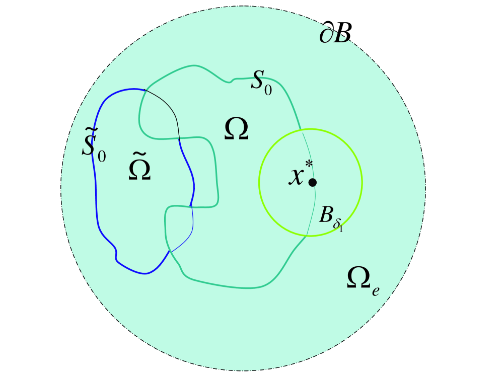
Fig. 2: Two different interfaces

Lemma 5.

If the electric far field patterns $E^{\infty}(\widehat{x},d,p)$ for $S_{0}$ and $\widetilde{E}^{\infty}(\widehat{x},d,q)$ for $\widetilde{S}_{0}$ coincide for all $\widehat{x},d,q\in S^{2}$, then the electric far field patterns also coincide for the incoming wave

$$E^{i}(x) = \frac{i}{k_{0}}{\rm curlcurl\,}\int_{S_{0}}s(y)\Phi_{0}(x,y)ds(y),$$ (3.1)

$$H^{i}(x) = {\rm curl\,}\int_{S_{0}}s(y)\Phi_{0}(x,y)ds(y),\qquad x\in B\cap\Omega_{e},$$ (3.2)

where $s\in T_{d}^{0,\alpha}(S_{0})$ has a compact support in $S_{0}\cap B_{\delta_{1}}$.

Proof.

By Rellich’s Lemma [8], the assumption $E^{\infty}(\hat{x};d,q)=\widetilde{E}^{\infty}(\hat{x};d,q)$ for all $\hat{x},d\in S^{2},\;q\in{\mathbb{R}}^{3}$ implies that $E^{s}(z,d,q)=\widetilde{E^{s}}(z,d,q)$ for all $z\in\Omega_{e}$ and all $d\in S^{2},\;q\in{\mathbb{R}}^{3}$. Using the mixed reciprocity relation (2.42), we obtain that the electric far field patterns corresponding to both interfaces coincide for incoming waves of the form

$$E^{i}(x;z,p) = \frac{i}{k_{0}}{\rm curlcurl\,}(p\Phi(x,z)),$$ (3.3)

$$H^{i}(x;z,p) = {\rm curl\,}(p\Phi_{0}(x,z)),\quad x\in\Omega_{e},\;x\neq z.$$ (3.4)

Furthermore, $E^{i}$ and $H^{i}$ defined as in (3.1) are continuous in $\overline{B\cap\Omega_{e}}$ and can be uniformly approximated, respectively, by fields of the form

$$E^{i}_{\delta_{2}}(x) = \frac{i}{k_{0}}{\rm curlcurl\,}\int_{S_{0}}s(y)\Phi_{0}(x+\delta_{2}\nu(x^{\ast}),y)ds(y),$$ (3.5)

$$H^{i}_{\delta_{2}}(x) = {\rm curl\,}\int_{S_{0}}s(y)\Phi_{0}(x+\delta_{2}\nu(x^{\ast}),y)ds(y),\qquad x\in\overline{B\cap\Omega_{e}}$$ (3.6)

by making $\delta_{2}$ sufficiently small. In fact, for $x\in(\overline{B\cap\Omega_{e}})\setminus B_{\delta_{1}}$ the differences between $E^{i}_{\delta_{2}}(x)$ and $E^{i}(x)$ and between $H^{i}_{\delta_{2}}(x)$ and $H^{i}(x)$ converge to zero as $\delta_{2}\rightarrow 0$ since $B_{\delta_{1}}\cap S_{0}-\delta_{2}\nu(x^{\ast})\subset\Omega$ for all sufficiently small $\delta_{2}>0$, so the kernels are smooth; for $x\in B_{\delta_{1}}$ the differences converge to zero since $E^{i}$ and $H^{i}$ are uniformly continuous in $\overline{B\cap\Omega_{e}}$ and $B_{\delta_{1}}\cap\Omega_{0}+\delta_{2}\nu(x^{\ast})\subset\Omega_{e}$ for all sufficiently small $\delta_{2}>0$.

Finally, with the help of a quadrature formula, the integrals in the definition of $E^{i}_{\delta_{2}}(x)$ and $H^{i}_{\delta_{2}}(x)$ can be uniformly approximated on $\overline{B\cap\Omega_{e}}$ by sums of waves of the form (3.3). Note that by the well-posedness of the direct problem we conclude that the electric far field pattern depends continuously on the incoming wave. Based on this result we obtain the assertion of the lemma. ∎

We are now ready to prove the main result of this section.

Lemma 6.

Let $\Im k_{1}>0$. If the electric far field patterns $E^{\infty}(\widehat{x},d,q)$ for $S_{0}$ and $\widetilde{E}^{\infty}(\widehat{x},d,q)$ for $\widetilde{S}_{0}$ coincide for all observation directions $\widehat{x}\in S^{2}$, all incident directions $d\in S^{2}$ and all polarizations $q\in{\mathbb{R}}^{3}$, then $S_{0}=\widetilde{S}_{0}$.

Proof.

We assume that $S_{0}\neq\widetilde{S}_{0}$. Then we can choose a point $x^{\ast}$ as we did at the beginning of Section 3. For the same $\delta_{1}$ as obtained there, we use a constant tangential vector $p\neq 0$ at $x^{\ast}$ and a smooth cut-off function $\rho$ that takes the value one close to $x^{\ast}$ and zero for $x$ with $|x-x^{\ast}|\geq\delta_{1}/3$. Define $x_{n}:=x^{\ast}+\delta_{1}/n\nu(x^{\ast})$, $n\in{\mathbb{N}}$. Denote by $E_{n},H_{n},F_{n},G_{n}$ the solution of the direct transmission problem (1.1)-(1.6) for the incoming wave:

$$E^{i}_{n}(x) = \lambda_{E}{\rm curlcurl\,}\int_{S_{0}}s_{n}(y)\Phi_{0}(x,y)ds(y),$$ (3.7)

$$H^{i}_{n}(x) = -ik_{0}\lambda_{E}{\rm curl\,}\int_{S_{0}}s_{n}(y)\Phi_{0}(x,y)ds(y),\qquad x\in B\cap\Omega_{e},\;\;n\in{\mathbb{N}},$$ (3.8)

where we set

$$s_{n}(x):=\frac{\rho(x)}{|x-x_{n}|^{1/2}}\nu(x)\times p,\qquad x\in S_{0},\;\;n\in{\mathbb{N}}.$$

Then define

$$F^{\ast}_{n}(x) := F_{n}(x)-{\rm curlcurl\,}\int_{S_{0}}s_{n}(y)\Phi_{1}(x,y)ds(y),$$

$$G^{\ast}_{n}(x) := G_{n}(x)+ik_{1}{\rm curl\,}\int_{S_{0}}s_{n}(y)\Phi_{1}(x,y)ds(y),\qquad x\in\Omega_{1},\;\;n\in{\mathbb{N}}$$

which satisfies the equations (1.2). Since $s_{n}$ is uniformly bounded in $T^{2}(S_{0})$ for all $n\in{\mathbb{N}}$, we have that

$$T^{\ast}_{1,n}(x) := \nu\times E_{n}-\lambda_{E}\nu\times F^{\ast}_{n}=\lambda_{E}(N_{0,1}-N_{0,0})Rs_{n},$$ (3.9)

$$T^{\ast}_{2,n}(x) := \nu\times H_{n}-\lambda_{E}\nu\times G^{\ast}_{n}=ik_{0}\lambda_{E}M_{0,0}s_{n}-ik_{1}\lambda_{H}M_{0,1}s_{n}$$ (3.10)

and ${\rm Div\,}T^{\ast}_{1,\;n}$ are uniformly bounded with respect to the $L^{2}(S_{0})-$norm. Consider the integral equations (2.21)-(2.25) in the space $T^{2}(S_{0})\times T^{2}(S_{0})\times T_{d}^{0,\alpha}(\Gamma_{1})\times T^{0,\alpha}(\Gamma_{2})\times C^{0,\alpha}(\Gamma_{2})$ with the right-hand sides $T^{\ast}_{1,\;n}(x)$ and $T^{\ast}_{2,\;n}(x)$ defined as above and

$$T^{\ast}_{3,n}(x) := \nu\times F^{\ast}_{n}=-N_{1,1}Rs_{n},\qquad x\in\Gamma_{1},$$

$$T^{\ast}_{4,n}(x) := \nu\times G^{\ast}_{n}-\frac{\lambda}{k_{1}}(\nu\times F^{\ast}_{n})\times\nu=ik_{1}M_{2,1}s_{n}-\frac{\lambda}{k_{1}}RN_{2,1}Rs_{n},\quad x\in\Gamma_{2}.$$

It can be found that the densities $a_{n}^{\ast},b_{n}^{\ast},c_{n}^{\ast},d_{n}^{\ast}$ and $\psi_{n}^{\ast}$ are uniformly bounded with respect to the norm of the above space. Using the regularity properties of the integral operators in (2.21) we conclude that the tangential fields $a_{n}^{\ast}$ are even uniformly bounded in $T_{d}^{2}(S_{0})$. Here, the condition $S_{0}\in C^{2,\alpha}$ is important since then we are able to use the fact that $M_{0,0}$ and $M_{0,1}$ map $T^{2}(S_{0})$ continuously into $T_{d}^{2}(S_{0})$ (see [13]). Let $B_{\delta_{1}/2}$ be the ball centered at $x^{\ast}$ with radius $\delta_{1}/2$ and define $\Gamma^{\ast}:=S_{0}\cap B_{\delta_{1}/2}$ and $\Gamma:=S_{0}\setminus B_{\delta_{1}/2}$. Then we have that ${\rm Div\,}T^{\ast}_{2,\;n}$ is uniformly bounded in $L^{2}(\Gamma)$. Thus, it follows from (2.22) that ${\rm Div\,}b_{n}^{\ast}$ is uniformly bounded in $L^{2}(\Gamma)$. These results together with the solution representation (2.13) imply that $\nu\times F^{\ast}_{n}$ is uniformly bounded with respect to the $T_{d}^{2}(\Gamma)-$norm.

By Lemma 5 and Rellich’s lemma $E_{n}$ and $H_{n}$ coincide with the scattered fields from the structure with interface $\widetilde{S}_{0}$. Since the incoming fields given by (3.7) are uniformly bounded on $\widetilde{S}_{0}$, $E_{n}$ and $H_{n}$ together with their derivatives are uniformly bounded in $B_{\delta_{1}/2}\subset\widetilde{\Omega_{0}}$. Hence, by the equation (3.9) and the regularity of $T^{\ast}_{1,\;n}$, $\nu\times F^{\ast}_{n}$ is also uniformly bounded with respect to the $T_{d}^{2}(\Gamma^{\ast})-$norm.

We now conclude by Lemma 7 below that ${\rm Div\,}(\nu\times G^{\ast}_{n})$ remains uniformly bounded in $L^{2}(S_{0})$ for all $n\in{\mathbb{N}}$. This implies that ${\rm Div\,}[\lambda_{H}\nu\times G_{n}-\nu\times H^{i}_{n}]=\lambda_{H}{\rm Div\,}(\nu\times G^{\ast}_{n})+{\rm Div\,}[\lambda_{H}\nu\times(G_{n}-G^{\ast}_{n})-\nu\times H^{i}_{n}]$ is uniformly bounded in $L^{2}(\Gamma)-$norm since $s_{n}$ is compactly supported in $B_{\delta_{1}/3}\cap S_{0}$ so the kernels in $\lambda_{H}\nu\times(G_{n}-G^{\ast}_{n})-\nu\times H^{i}_{n}$ are smooth. Furthermore, The function ${\rm Div\,}[\lambda_{H}\nu\times G_{n}-\nu\times H^{i}_{n}]={\rm Div\,}(\nu\times H_{n})$ is also uniformly bounded in $L^{2}(\Gamma^{\ast})-$norm since $H_{n}$ and its derivatives are uniformly bounded in $B_{\delta_{1}/2}$. By the vector identity ${\rm Div\,}(\nu\times V)=-\nu\cdot{\rm curl\,}V$ we conclude that the fields

$${\rm Div\,}[\lambda_{H}\nu\times(G_{n}-G^{\ast}_{n})-\nu\times H^{i}_{n}]$$

$$= {\rm Div\,}[-ik_{1}\lambda_{H}\nu\times{\rm curl\,}\int_{S_{0}}s_{n}(y)\Phi_{1}(x,y)ds(y)$$

$$+ik_{0}\lambda_{E}\nu\times{\rm curl\,}\int_{S_{0}}s_{n}(y)\Phi_{0}(x,y)ds(y)]$$

$$= -ik_{1}\lambda_{H}\nu\cdot{\rm curlcurl\,}\int_{S_{0}}s_{n}(y)\Phi_{1}(x,y)ds(y)$$

$$+ik_{0}\lambda_{E}\nu\cdot{\rm curlcurl\,}\int_{S_{0}}s_{n}(y)\Phi_{0}(x,y)ds(y)$$

remains uniformly bounded in $L^{2}(S_{0})$. Thus, denoting by $\widetilde{\Phi}_{0}$ the fundamental solution of the Laplace equation, we have that

$$\lim_{\epsilon\rightarrow 0,\;\epsilon>0}\nu\cdot{\rm curlcurl\,}\int_{S_{0}}s_{n}(y)\widetilde{\Phi}_{0}(x+\epsilon\nu(x),y)ds(y)$$

$$= \lim_{\epsilon\rightarrow 0,\;\epsilon>0}\frac{\partial}{\partial\nu(x)}{\rm div}\int_{S_{0}}s_{n}(y)\widetilde{\Phi}_{0}(x+\epsilon\nu(x),y)ds(y)$$

is uniformly bounded in $L^{2}(S_{0})$. Here we have used the identity ${\rm curlcurl\,}V=-\Delta V+\nabla{\rm div}V$ and the fact that $k_{0}\lambda_{E}-k_{1}\lambda_{H}=k^{2}_{0}(1+k^{2}_{1}\lambda_{H}^{2})/({k_{1}\lambda_{H}})\neq 0$ since $k_{0},\;\Re k_{1},\;\Im k_{1}$ and $\lambda_{H}$ are positive constants. From this we conclude that

$$f_{n}(x)={\rm Div\,}s_{n}(x)+2\int_{S_{0}}{\rm Div\,}s_{n}(y)\frac{\partial\Phi_{1}}{\partial\nu(x)}(x,y)ds(y),\qquad x\in S_{0}$$

is uniformly bounded in $L^{2}(S_{0})$. Consequently, ${\rm Div\,}s_{n}$ remains uniformly bounded in $L^{2}(S_{0})$ for all $n\in{\mathbb{N}}$ since the above integral equation is uniquely solvable in $L^{2}(S_{0})$ and the inverse operator is continuous in $L^{2}(S_{0})$. Computing ${\rm Div\,}s_{n}$ and omitting the terms that are obviously uniformly bounded in $L^{2}(S_{0})$ we have that

$$\frac{(\nu(x)\times p)\cdot(x-x^{\ast})}{|x-x^{\ast}|^{5/2}},\qquad x\in S_{0}$$

is uniformly bounded in $L^{2}(S_{0})$. This is a contradiction as can be seen by parameterizing $S_{0}$ locally around $x^{\ast}$. This ends the proof. ∎

It remains to prove the following lemma.

Lemma 7.

Let $\Im k_{1}>0$. Assume that $T_{1,n}\in T_{d}^{0,\alpha}(S_{0})$ is uniformly bounded in $T_{d}^{2}(S_{0})$, $T_{3,n}$ is uniformly bounded in $T_{d}^{0,\alpha}(\Gamma_{1})$ and $T_{4,n}$ is uniformly bounded in $T^{0,\alpha}(\Gamma_{2})$ for all $n\in{\mathbb{N}}$. Then there exists a unique solution $F^{\ast}_{n},\;G^{\ast}_{n}\in C^{1}(\Omega_{1})\cap C(\overline{\Omega_{1}})$ to the Maxwell equations

$${\rm curl\,}F^{\ast}_{n}-ik_{1}G^{\ast}_{n}=0,\qquad{\rm curl\,}G^{\ast}_{n}+ik_{1}F^{\ast}_{n}=0\qquad{\rm in}\;\;\Omega_{1}$$

with boundary conditions

$$\nu\times F^{\ast}_{n}=T_{1,n}\qquad {\rm on}\;\;S_{0},$$

$$\nu\times F^{\ast}_{n}=T_{3,n}\qquad {\rm on}\;\;\Gamma_{1},$$

$$\nu\times G^{\ast}_{n}-\frac{\lambda}{k_{1}}[\nu\times F^{\ast}_{n}]\times\nu=T_{4,n}\qquad {\rm on}\;\;\Gamma_{2}$$

for each $n\in{\mathbb{N}}$. Furthermore, ${\rm Div\,}(\nu\times G^{\ast}_{n})$ is uniformly bounded in $L^{2}(S_{0})$ for all $n\in{\mathbb{N}}$.

Proof.

We first prove the uniqueness result. Let $T_{1,n}=0$ on $S_{0}$, $T_{3,n}=0$ on $\Gamma_{1}$ and $T_{4,n}=0$ on $\Gamma_{2}$. Then we just need to prove that $F^{\ast}_{n}=G^{\ast}_{n}=0$ in $\Omega_{1}$. Using Green’s vector theorem and the above Maxwell equations, we have

$$0 = k_{1}\int_{\Omega_{1}}\{{\rm curl\,}G^{\ast}_{n}\cdot\overline{F^{\ast}_{n}}+ik_{1}F^{\ast}_{n}\cdot\overline{F^{\ast}_{n}}\}dx$$

$$= k_{1}\int_{\Omega_{1}}\{G^{\ast}_{n}\cdot{\rm curl\,}\overline{F^{\ast}_{n}}+ik_{1}|F^{\ast}_{n}|^{2}\}dx-\int_{\Gamma_{2}}\lambda|\nu\times F^{\ast}_{n}|^{2}ds$$

$$= \int_{\Omega_{1}}\{-i|k_{1}G^{\ast}_{n}|^{2}+i[(\Re k_{1})^{2}-(\Im k_{1})^{2}]|F^{\ast}_{n}|^{2}-2\Re k_{1}\Im k_{1}|F^{\ast}_{n}|^{2}\}dx-\int_{\Gamma_{2}}\lambda|\nu\times F^{\ast}_{n}|^{2}ds$$

Taking the real part of the above equation and noting that $\Im k_{1}>0$, we get $F^{\ast}_{n}=G^{\ast}_{n}=0$ in $\Omega_{1}$.

To prove the existence, we seek a solution in the form

$$F^{\ast}_{n}(x) = {\rm curl\,}\int_{S_{0}}a_{n}(y)\Phi_{1}(x,y)ds(y)$$ (3.14)

$$+{\rm curl\,}\int_{\Gamma_{1}}c_{n}(y)\Phi_{1}(x,y)ds(y)+\frac{i}{k_{1}^{2}}{\rm curlcurl\,}\int_{\Gamma_{1}}\nu(y)\times(\widehat{S}_{1}^{2}c_{n})(y)\Phi_{1}(x,y)ds(y)$$

$$+\int_{\Gamma_{2}}d_{n}(y)\Phi_{1}(x,y)ds(y)+i\lambda{\rm curl\,}\int_{\Gamma_{2}}\nu(y)\times(\widehat{S}_{2}^{2}d_{n})(y)\Phi_{1}(x,y)ds(y)$$

$$+{\rm grad}\int_{\Gamma_{2}}\psi_{n}(y)\Phi_{1}(x,y)ds(y)+i\lambda\int_{\Gamma_{2}}\nu(y)\psi_{n}(y)\Phi_{1}(x,y)ds(y),$$

$$G^{\ast}_{n}(x) = \frac{1}{ik_{1}}{\rm curl\,}F^{\ast}_{n}(x)$$ (3.15)

for $x\in\Omega\setminus S_{1}$. The jump relations together with the regularity of the surface potentials imply that $F^{\ast}_{n},\;G^{\ast}_{n}$ defined in (3.14)-(3.15) solve the mixed boundary problem in $\Omega_{1}$ provided the densities $a_{n},\;c_{n},\;d_{n},\;\psi_{n}$ satisfy

$$-a_{n}+M_{0,1}a_{n}-\frac{1}{\lambda_{E}}N_{1}c_{n}-\frac{1}{\lambda_{E}}P_{1}d_{n}-\frac{1}{\lambda_{E}}Q_{1}\psi_{n} = 2T_{1,n}\qquad{\rm on}\;\;S_{0},$$ (3.16)

$$c_{n}+L_{3}a_{n}+N_{3}c_{n}+P_{3}d_{n}+Q_{3}\psi_{n} = 2T_{3,n}\qquad{\rm on}\;\;\Gamma_{1},$$ (3.17)

$$d_{n}+L_{4}a_{n}+N_{4}c_{n}+P_{4}d_{n}+Q_{4}\psi_{n} = 2T_{4,n}\qquad{\rm on}\;\;\Gamma_{2},$$ (3.18)

$$i\lambda\psi_{n}+P_{5}d_{n}+Q_{5}\psi_{n} = 0\qquad\qquad{\rm on}\;\;\Gamma_{2}.$$ (3.19)

This system of integral equations is Fredholm in $Y:=T^{2}(S_{0})\times T_{d}^{0,\alpha}(\Gamma_{1})\times T^{0,\alpha}(\Gamma_{2})\times C^{0,\alpha}(\Gamma_{2})$. Therefore we just need to prove that the corresponding homogeneous system has a trivial solution. Similar to the argument in the proof of Theorem 2, we can prove that $\psi_{n}=0$ on $\Gamma_{2}$, $c_{n}=0$ on $\Gamma_{1}$ and $d_{n}=0$ on $\Gamma_{2}$. Note that $F^{\ast}_{n},G^{\ast}_{n}$ are also well-defined in $\Omega_{0}$ and are a radiation solution to the Maxwell equations

$${\rm curl\,}F^{\ast}_{n}-ik_{1}G^{\ast}_{n}=0,\qquad{\rm curl\,}G^{\ast}_{n}+ik_{1}F^{\ast}_{n}=0\qquad\mbox{in}\;\;\Omega_{0}$$

with the homogenous boundary condition

$$\nu\times F^{\ast}_{n}=0\qquad\mbox{on}\;\;S_{0}.$$

Thus, by Theorem 6.18 in [8] we obtain that $F^{\ast}_{n}=0$ in $\Omega_{0}$. By the jump relations, we have

$$-a_{n}+M_{0,1}a_{n}=0=a_{n}+M_{0,1}a_{n}\qquad{\rm on}\;\;S_{0},$$

so $a_{n}=0$ on $S_{0}$.

Since the right-hand side of the system of integral equations (3.16)-(3.19) is bounded in $Y$, then the solution $a,c,d,\psi$ is also bounded in $Y$. Thus, using the integral representation (3.14) and by Lemma 1 in [11], ${\rm Div\,}(\nu\times G^{\ast}_{n})=-\nu\cdot{\rm curl\,}G^{\ast}_{n}=ik_{1}\nu\cdot F^{\ast}_{n}$ is uniformly bounded in $L^{2}(S_{0})$ for all $n\in{\mathbb{N}}$. This proves the lemma. ∎

4 Unique determination of the boundary $S_{1}$ and its property

In this section we will prove that, given that $S_{0}=\widetilde{S}_{0}$, the impenetrable obstacle $\Omega_{2}$ and its physical property $\mathscr{B}$ can be uniquely determined. Note that in this problem we only assume that the wave number $k_{1}$ can be any constant with $\Im k_{1}\geq 0$, so the result obtained in this section is a generalization of that in [20].

Lemma 8.

For $\Omega_{2},\widetilde{\Omega}_{2}\subset\Omega$, let $G$ be the unbounded component of ${\mathbb{R}}^{3}\setminus(\overline{\Omega_{2}\cup\widetilde{\Omega}_{2}})$ and let $E^{\infty}(\hat{x};d,q)=\widetilde{E}^{\infty}(\hat{x};d,q)$ for all $\hat{x},d\in S^{2},\;q\in{\mathbb{R}}^{3}$ with $\widetilde{E}^{\infty}(\hat{x};d,q)$ being the electric far field pattern of the scattered field $\widetilde{E}^{s}(x;d,q)$ corresponding to the obstacle $\widetilde{\Omega}_{2}$ and the same incident plane wave $E^{i}(\hat{x};d,q)$. Let $z\in\Omega_{1}\cap G,$ $E^{i}=E^{i}(x;z,p),\;H^{i}=H^{i}(x;z,p)$ and let $F=F(x;z,p)$ be the unique solution of the problem

$${\rm curl\,}E-ik_{0}H=0\;\;{\rm curl\,}H+ik_{0}E=0\qquad {\rm in}\;\;\Omega_{0},$$ (4.1)

$${\rm curl\,}F-ik_{1}G=0\;\;{\rm curl\,}G+ik_{1}F=0\qquad {\rm in}\;\;\Omega_{1},$$ (4.2)

$$\nu\times E-\lambda_{E}\nu\times F=\lambda_{E}\nu\times E^{i},\;\;\nu\times H-\lambda_{H}\nu\times G=\lambda_{H}\nu\times H^{i}\qquad {\rm on}\;\;S_{0},$$ (4.3)

$$\nu\times F=-\nu\times E^{i}\qquad {\rm on}\;\;\Gamma_{1},$$ (4.4)

$$\nu\times G-\frac{\lambda}{k_{1}}(\nu\times F)\times\nu=-\nu\times H^{i}+\frac{\lambda}{k_{1}}(\nu\times E^{i})\times\nu\qquad {\rm on}\;\;\Gamma_{2},$$ (4.5)

$$\lim_{|x|\rightarrow\infty}(H\times x-|x|E)=0.\qquad$$ (4.6)

Let $\widetilde{F}$ =$\widetilde{F}(x;z,p)$ be the unique solution of the above problem with $\Omega_{2}$ replaced by $\widetilde{\Omega_{2}}$ and $\Omega_{1}$ replaced by $\widetilde{\Omega_{1}}:=\Omega\backslash(\overline{\Omega_{1}})$. Then

$$F(x;z,p)=\widetilde{F}(x;z,p),\qquad\forall\;x\in\Omega_{1}\cap G.$$ (4.7)

Remark 9.

By Theorem 2, the problem (4.1)-(4.6) has a unique solution.

Proof.

By Rellich’s Lemma [8], the assumption that $E^{\infty}(\hat{x};d,q)=\widetilde{E}^{\infty}(\hat{x};d,q)$ for all $\hat{x},d\in S^{2},\;q\in{\mathbb{R}}^{3}$ implies that

$$\nu\times E(x,d,q)=\nu\times\widetilde{E}(x,d,q),\qquad\nu\times H(x,d,q)=\nu\times\widetilde{H}(x,d,q)$$

for all $x\in S_{0}$ and all $d\in S^{2},\;q\in{\mathbb{R}}^{3}$. By Holmgren’s uniqueness theorem (see Lemma 3.2 in [2] or Theorem 4.1.2.4 in [15]), it follows that

$$\widetilde{F}(z,d,q)=F(z,d,q),\qquad\forall\;d\in S^{2},\;q\in{\mathbb{R}}^{3}.$$

For the electric far field patterns corresponding to the electric dipole we have by the mixed reciprocity relation (2.43) that

$$E^{\infty}(d;z,p)=\widetilde{E}^{\infty}(d;z,p),\qquad\forall\;d\in S^{2},\;q\in{\mathbb{R}}^{3}.$$

Rellich’s Lemma [8] gives

$$\nu\times E(x;z,p)=\nu\times\widetilde{E}(x;z,p),\quad\nu\times H(x;z,p)=\nu\times\widetilde{H}(x;z,p)$$

for all $x\in S_{0},\;p\in{\mathbb{R}}^{3}$. By Holmgren’s uniqueness theorem again it is derived that

$$\widetilde{F}(x;z,p)=F(x;z,p),\qquad\forall\;x\in\Omega_{1}\cap G,\;p\in{\mathbb{R}}^{3},$$

which is the desired result (4.7). ∎

Making use of Lemma 8 and the mixed reciprocity relation (2.43) we can prove the following uniqueness result.

Theorem 10.

If there are two obstacles $\Omega_{2}$ and $\widetilde{\Omega}_{2}$ which lead to the same far field pattern for all observation directions and all incident directions at a fixed frequency, i.e., $E^{\infty}(\widehat{x},d,q)=\widetilde{E}^{\infty}(\widehat{x},d,q)$ for all $\widehat{x},\;d\in S^{2}$ and all $q\in{\mathbb{R}}^{3}$, then $S_{1}=\widetilde{S}_{1}$ and $\mathscr{B}=\widetilde{\mathscr{B}}$, that is, the impenetrable obstacle with its physical property are uniquely determined.

Proof.

Let G be the unbounded component of ${\mathbb{R}}^{3}\setminus(\overline{\Omega_{2}\cup\widetilde{\Omega}_{2}})$. Assume that $S_{1}\neq\widetilde{S}_{1}$. Then, without loss of generality, we may assume that there exists a point $z_{0}\in S_{1}\cap\left({\mathbb{R}}^{3}\backslash\overline{\widetilde{\Omega}_{2}}\right)$. We can choose an $h>0$ such that the sequence

$$z_{j}:=z_{0}+\frac{h}{j}\nu(z_{0}),\qquad j=1,2,\ldots,$$

is contained in $G$, where $\nu(z_{0})$ is the outward normal to $S_{1}$ at $z_{0}$. Consider the solution to the problem (4.1)-(4.6) with $z$ being replaced by $z_{j}$. By Lemma 8 it follows that $E^{s}(x;z_{j},p)=\widetilde{E}^{s}(x;z_{j},p)$ for all $x\in\overline{G}$ and all polarizations $p\in{\mathbb{R}}^{3}$. Since $z_{0}$ has a positive distance from $\overline{\widetilde{\Omega}_{2}}$, we conclude from the well-posedness of the direct problem that there exists a $C>0$ such that $|\mathscr{B}(\widetilde{E}^{s}(z_{0};z_{j},p))|\leq C$ uniformly for $j\geq 1$ and all polarizations $p\in{\mathbb{R}}^{3}$. On the other hand, by the boundary condition on $S_{1}$,

$$|\mathscr{B}(\widetilde{E}^{s}(z_{0};z_{j},p))|=|\mathscr{B}(E^{s}(z_{0};z_{j},p))|=|-\mathscr{B}(E^{i}(z_{0},z_{j},p))|\rightarrow\infty$$

as $j\rightarrow\infty$ for $p\,\bot\,\nu(z_{0})$. This is a contradiction and therefore $S_{1}=\widetilde{S}_{1}$.

We now assume that the boundary conditions are different, that is, $\mathscr{B}\neq\widetilde{\mathscr{B}}$. Since the obstacles and the far field patterns are the same, we have $F(x,d,q)=\widetilde{F}(x,d,q)$. Define $\Omega_{2}:=\Omega_{2}=\widetilde{\Omega}_{2}$ and $F:=F(x,d,q)=\widetilde{F}(x,d,q)$ and consider the case of impedance boundary conditions with two different positive constants $\lambda\neq\widetilde{\lambda}$. Then from the boundary conditions

$$\nu\times G-\frac{\lambda}{k_{1}}(\nu\times F)\times\nu=0,\;\;\nu\times G-\frac{\widetilde{\lambda}}{k_{1}}(\nu\times F)\times\nu=0\qquad{\rm on}\;S_{1},$$ (4.8)

we observe that

$$(\lambda-\widetilde{\lambda})\nu\times F=0\qquad{\rm on}\;\;S_{1}.$$

This, together with the boundary conditions (4.8), implies that $\nu\times F=\nu\times G=0$ on $S_{1}$. Therefore, by Holmgren’s uniqueness theorem [2, 15], $F=G=0$ in $\Omega_{1}$. Using Holmgren’s uniquness theorem again and with the help of the transmission boundary conditions, we conclude that $E(x,d,q)=E^{i}(x,d,q)+E^{s}(x,d,q)=0$ in $\Omega_{0}$. The scattered field $E^{s}(x,d,q)$ tends to zero uniformly at infinity, while the incident plane wave $E^{i}(x,d,q)$ has modulus $|k_{0}(d\times q)\times d|$ everywhere. Thus the modulus of the total field tends to $|k_{0}(d\times q)\times d|$. This leads to a contradiction, giving that $\lambda=\widetilde{\lambda}$. The cases with other boundary conditions can be dealt with similarly. ∎

We summarize the main results for the inverse problem in the following theorem.

Theorem 11.

Let $\Im k_{1}>0$. Then the interface $S_{0}$ and the obstacle $\Omega_{2}$ with its physical property $\mathscr{B}$ are uniquely determined by the electric far field patterns $E^{\infty}(\widehat{x},d,q)$ for all observation directions $\widehat{x}\in S^{2}$, all incident directions $d\in S^{2}$ and all polarizations $q\in{\mathbb{R}}^{3}$.

There is a widespread belief that the electric far field pattern for a single incident direction $d\in S^{2}$ and a single polarization direction $q$ uniquely determines the general obstacle, since the far field data depend on the same number of variables, as does the obstacle to be recovered. However, this result remains a challenging open problem [4]. Recent progress has been made by Liu, Zhang & Zou [18] who established uniqueness with a single incident wave for a polyhedral obstacle and by Kress [17] who proved that a ball and its boundary condition (for constant impedance $\lambda$) are uniquely determined by the far field pattern for one incident plane wave. In a recent paper [10], we proved uniqueness in determining a small perfectly conducting ball in the inverse electromagnetic scattering problem by a finite number of electric far field patterns with a single incident direction and polarization. We now extend Kress’s result to our case that the background is a piecewise homogeneous medium.

Corollary 12.

Let $\Im k_{1}>0$. Assume that the interface $S_{0}$ and the boundary $S_{1}$ are concentric spheres with center at the origin and the impedance $\lambda$ is a positive constant. Then they are uniquely determined by the electric far field patterns $E^{\infty}(\widehat{x},d,q)$ for all observation directions $\widehat{x}\in S^{2}$, one fixed incident direction $d\in S^{2}$ and all polarizations $q\in{\mathbb{R}}^{3}$.

Proof.

By symmetry, the electric far field pattern for scattering of plane waves by the concentric spheres $S_{0}$ and $S_{1}$ and the positive constant impedance $\lambda$ satisfies $E^{\infty}(Q\widehat{x},Qd,Qq)=QE^{\infty}(\widehat{x},d,q)$ for all $\widehat{x},d\in S^{2}$, $q\in{\mathbb{R}}^{3}$ and all rotations $Q$, that is, for all orthogonal transformations with $\det Q=1$. Hence, knowledge of the electric far field pattern for one incident direction implies knowledge of the electric far field pattern for all incident directions. The statement now follows from Theorem 11. ∎

Karp’s theorem in our case as stated in the following corollary is also true.

Corollary 13.

Let $\Im k_{1}>0$. Assume that the electric far field patterns $E^{\infty}(\widehat{x},d,q)$ satisfies $E^{\infty}(Q\widehat{x},Qd,Qq)=QE^{\infty}(\widehat{x},d,q)$ for all $\widehat{x},d\in S^{2}$, $q\in{\mathbb{R}}^{3}$ and all orthogonal transformations $Q$ with $\det Q=1$. Then the interface $S_{0}$ and the boundary $S_{1}$ are concentric spheres with center at the origin.

Proof.

We define $\widetilde{S}_{0}=Q(S_{0})$ and $\widetilde{S}_{1}=Q(S_{1})$ for some orthogonal transformation $Q$ with $\det Q=1$. Then, by symmetry the corresponding electric far field pattern $\widetilde{E}^{\infty}(\widehat{x},d,q)$ for $\widetilde{S}_{0},\;\widetilde{S}_{1}$ satisfies

$$\widetilde{E}^{\infty}(\widehat{x},d,q)=QE^{\infty}(Q^{-1}\widehat{x},Q^{-1}d,Q^{-1}q)=E^{\infty}(\widehat{x},d,q)$$

for all $\widehat{x},d\in S^{2}$, $q\in{\mathbb{R}}^{3}$. Theorem 11 implies that $\widetilde{S}_{0}=S_{0}$ and $\widetilde{S}_{1}=S_{1}$. This holds for all orthogonal transformations $Q$. Therefore $S_{0}$ and $S_{1}$ are concentric spheres with center at the origin. ∎

References

- [1] C. Athanasiadis, Scattering theorems for time-harmonic electromagnetic waves in a piecewise homogeneous medium, Math. Proc. Camb. Phil. Soc. 123 (1998), 179-190.
- [2] T. Abboud and J.C. Nedelec, Electromagnetic waves in an inhomogeneous medium, J. Math. Anal. Appl. 164 (1992), 40-58.
- [3] F. Cakoni and D. Colton, The determination of the surface impedance of a partially coated obstacle from far field data, SIAM J. Appl. Math. 64 (2004), 709-723.
- [4] F. Cakoni and D. Colton, Open problems in the qualitative approach to inverse electromagnetic scattering theory, Europ. J. Appl. Math. 16 (2005), 411-425.
- [5] F. Cakoni, D. Colton and P. Monk, The electromganetic inverse scattering problem for partially coated Lipschitz Domains, Proc. Roy. Soc. Edinburgh 134 A (2004), 661-682.
- [6] F. Cakoni and D. Colton, and P. Monk, The determination of the surface conductivity of a partially coated dielectric, SIAM J. Appl. Math. 65 (2005), 767-789.
- [7] D. Colton and R. Kress, Integral Equation Methods in Scattering Theory, Wiley, New York, 1983.
- [8] D. Colton and R. Kress, Inverse Acoustic and Electromagnetic Scattering Theory (Second Edition), Springer, Berlin, 1998.
- [9] F. Hettlich, Uniqueness of the inverse conductive scattering problem for time-harmonic electromagnetic waves, SIAM J. Appl. Math. 56 (1996), 588-601.
- [10] G. Hu, X. Liu and B. Zhang, Unique determination of a perfectly conducting ball by a finite number of electric far field data, J. Math. Anal. Appl. 352 (2009), 861-871.
- [11] P. Hähner, A uniqueness theorem for a transmission problem in inverse electromagnetic scattering, Inverse Problems 9 (1993), 667-678.
- [12] V. Isakov, On uniqueness in the inverse transmission scattering problem, Commun. Partial Differential Equations 15 (1990), 1565-1587.
- [13] A. Kirsch, Surface gradients and continuity properties for some integral operators in classical scattering theory, Math. Meth. Appl. Sci. 11 (1989), 789-804.
- [14] A. Kirsch and R. Kress, Uniqueness in inverse obstacle scattering, Inverse Problems 9 (1993), 285-299.
- [15] R. Kress, Electromagnetic waves scattering: Specific theoretical tools. In: Scattering (R. Pike, P. Sabatier, eds.), Academic Press, London, 2001, pp. 175-190.
- [16] R. Kress, Electromagnetic waves scattering: Scattering by obstacles. In: Scattering (R. Pike, P. Sabatier, eds.), Academic Press, London, 2001, pp. 191-210.
- [17] R. Kress, Uniqueness in inverse obstacle scattering for electromagnetic waves, in: Proceedings of the URSI General Assembly, 2002, Maastricht.
- [18] H. Liu, H. Zhang and J. Zou, Recovery of polyhedral scatterers by a single electromagnetic far-field measurement, J. Math. Phys. 50 (2009), 123506.
- [19] X. Liu, B. Zhang and G. Hu, Uniqueness in the inverse scattering problem in a piecewise homogeneous medium, Inverse Problems 26 (2010), 015002.
- [20] X. Liu, B. Zhang, A uniqueness result for the inverse electromagnetic scattering problem in a piecewise homogeneous medium, Applicabel Analysis 88 (2009), 1339-1355.
- [21] X. Liu, B. Zhang, Direct and inverse obstacle scattering problems in a piecewise homogeneous medium, submitted for publication, 2009 (arXiv:0912.1443v1).
- [22] X. Liu, B. Zhang, Inverse scattering by an inhomogeneous penetrable obstacle in a piecewise homogeneous medium, submitted for publication, 2009 (arXiv:0912.2788v1).