High-Resolution Spectroscopy of Extremely Metal-Poor Stars in the Least Evolved Galaxies: Leo IV

Abstract

We present high-resolution Magellan/MIKE spectroscopy of the brightest star in the ultra-faint dwarf galaxy Leo IV. We measure an iron abundance of $\rm{[Fe/H]}=-3.2$, adding to the rapidly growing sample of extremely metal-poor stars being identified in Milky Way satellite galaxies. The star is enhanced in the $\alpha$ elements Mg, Ca, and Ti by $\sim 0.3$ dex, very similar to the typical Milky Way halo abundance pattern. All of the light and iron-peak elements follow the trends established by extremely metal-poor halo stars, but the neutron-capture elements Ba and Sr are significantly underabundant. These results are quite similar to those found for stars in the ultra-faint dwarfs Ursa Major II, Coma Berenices, Boötes I, and Hercules, suggesting that the chemical evolution of the lowest luminosity galaxies may be universal. The abundance pattern we observe is consistent with predictions for nucleosynthesis from a Population III supernova explosion. The extremely low metallicity of this star also supports the idea that a significant fraction ($\gtrsim 10$%) of the stars in the faintest dwarfs have metallicities below $\rm{[Fe/H]}=-3.0$.

1. INTRODUCTION

The chemical abundance patterns of the most metal-poor stars provide a unique fossil record of star formation, chemical evolution, and supernova nucleosynthesis in the early universe. Until recently, such studies were limited to the stellar halo of the Milky Way because nearby dwarf galaxies appeared to lack sufficiently metal-poor stars (Helmi et al., 2006). Just over a year ago, the first extremely metal-poor (EMP) stars with $\rm{[Fe/H]}\leq-3.0$ were discovered in several of the Milky Way’s lowest luminosity companions (Kirby et al., 2008). Since then, the number of known EMP stars in nearby dwarf galaxies has been expanding rapidly (Frebel et al., 2010a; Cohen & Huang, 2009; Aoki et al., 2009; Frebel, Kirby, & Simon, 2010b; Norris et al., 2009).

Because the ultra-faint dwarfs host such incredibly tiny stellar populations ($L\lesssim 10^{4}$ L_⊙), they represent particularly attractive targets for chemical abundance studies. These galaxies should have hosted only a few supernovae (SNe), and the individual chemical signatures of those explosions may be revealed in their oldest stars (e.g., Koch et al., 2008). Moreover, they were likely some of the first objects to collapse in the early universe (Bovill & Ricotti, 2009), and the lack of star formation at later times means that evidence of the nucleosynthetic processes operating at high redshift should be preserved.

In a previous paper we presented high-resolution spectra of six stars in the ultra-faint dwarfs Ursa Major II (UMa II) and Coma Berenices (ComBer), showing that both galaxies have very low metallicities, substantial iron abundance spreads, and overall abundance patterns similar to that of the Milky Way halo (Frebel et al., 2010a). Here we report spectroscopy of the brightest star (and the only one accessible to current telescopes at high spectral resolution) in the slightly more luminous galaxy Leo IV. In § 2 we describe Leo IV and our observations. We present our abundance analysis in §3, and then discuss the implications of our results for the chemical evolution of the faintest galaxies in § 4. In § 5 we briefly summarize our findings and conclude.

2. OBSERVATIONS AND DATA REDUCTION

2.1. Properties of Leo IV

Leo IV was discovered as an overdensity of resolved stars in the fifth data release of the Sloan Digital Sky Survey (Adelman-McCarthy et al., 2007) by Belokurov et al. (2007). Medium-resolution spectroscopy by Simon & Geha (2007, hereafter SG07) demonstrated that Leo IV has stellar kinematics and metallicities that are characteristic of dwarf galaxies, but as the most poorly-studied object in the SG07 sample its overall properties were not well constrained. Followup analysis of the SG07 spectra by Kirby et al. (2008) revealed that Leo IV has the lowest mean metallicity of any galaxy known, at $\rm{[Fe/H]}=-2.58\pm 0.08$, with a very large internal metallicity spread of 0.75 dex. Subsequently, photometric studies by Martin, de Jong, & Rix (2008), Sand et al. (2009), Moretti et al. (2009), and de Jong et al. (2010) refined the size ($128\pm 26$ pc), absolute magnitude ($M_{V}=-5.7\pm 0.3$), and distance ($154\pm 5$ kpc) of the galaxy. SG07 identified a single bright red giant star, SDSSJ113255.99–003027.8 (hereafter referred to as Leo IV-S1), in Leo IV at $V=19.2$, with the next brightest confirmed member nearly a magnitude fainter.

2.2. Observations

We observed Leo IV-S1 on 2009 February 18–20 with the Magellan Inamori Kyocera Echelle (MIKE) spectrograph (Bernstein et al., 2003) on the Clay Telescope. The observations were made with a 1″ slit, producing a spectral resolution of $R=28,000$ on the blue side ($\lambda<5000$ Å) and a resolution of $R=22,000$ on the red side ($\lambda>5000$ Å). The CCD was binned $3\times 3$ to reduce read noise for such a faint target, yielding a final dispersion of $\sim 0.07$ Å pixel^-1 in the blue and $\sim 0.12$ Å pixel^-1 in the red (i.e., sampling slightly better than the Nyquist rate). A temporary, lower efficiency detector was used because of the failure of the MIKE blue CCD in 2008 November. The total integration time was 8.67 hours (individual exposures were either 40 or 55 minutes) under mostly excellent observing conditions.

2.3. Data Reduction

The data were reduced using the latest version of the MIKE pipeline introduced by Kelson (2003). Frames from each night were reduced together, and then the spectra from the individual nights were coadded at the end. The final spectrum was normalized in IRAF and each order was analyzed separately. Because of the target star’s faintness, the signal-to-noise ratio (S/N) achieved is modest: $\rm{S/N}=10$ pixel^-1 at 4500 Å, $\rm{S/N}=25$ pixel^-1 at 5500 Å, and $\rm{S/N}=45$ pixel^-1 at 6500 Å, comparable to that obtained for similarly faint stars by Koch et al. (2008) and Koch, Côté, & McWilliam (2009). We measure a velocity of $130.9\pm 1.1$ km s^-1, consistent with the previous measurement of $132.7\pm 2.2$ km s^-1 from SG07, which suggests that Leo IV-S1 does not have a binary companion in a close enough orbit to affect its evolution or abundances.

3. ABUNDANCE ANALYSIS

3.1. Line Measurements and Atmospheric Parameters

Using a line list taken from McWilliam et al. (1995a) and Frebel et al. (2010a), we measured equivalent widths (EWs) with the IRAF task splot. We detected $\sim 50$ Fe I lines, and between one and ten lines for the following species: Fe II, Mg I, Ca I, Sc II, Ti I, Ti II, Na I, Cr I, Ni I, Sr II, and Ba II. A portion of the spectrum illustrating the detection of Ba is displayed in Figure 1, and the EWs of all measured lines are listed in Table 1.

Based on a combined photometric and spectroscopic analysis, Kirby et al. (2008) estimated $T_{eff}=4330$ K, $\log{g}=1.0$, $\xi=1.6$ km s^-1, and $\rm{[Fe/H]}=-2.9$ for Leo IV-S1. Starting with these parameters, we constructed a 1D plane-parallel Kurucz model atmosphere (Kurucz, 1992) and then iteratively redetermined the stellar parameters using the Fe I lines with the 2009 version of MOOG (Sneden, 1973). We first established the microturbulent velocity by minimizing the trend of Fe I abundance with EW. The derived value was $\xi=3.2$ km s^-1, which would be quite high for the less luminous stars that are frequently observed in the Milky Way halo and globular clusters, but is comparable to values obtained for cool EMP giants from low S/N spectra in a number of other studies (McWilliam et al., 1995a; Koch et al., 2008; Aoki et al., 2009; Frebel et al., 2010b).

Next, we determined the effective temperature. Leo IV-S1 is unfortunately too faint to have been detected by 2MASS, so the reddest available color is $V-I$ (converted from the SDSS magnitudes using the Jordi et al. 2006 transformations). The color-temperature relation of Alonso et al. (1999) predicts $T_{eff}=4330$ K using either $B-V$ (from Moretti et al. 2009) or $V-I$. At this temperature, there is still a weak negative trend of Fe I abundance with excitation potential, as noted for similar stars by Norris et al. (2009, and references therein), perhaps indicating deviations from local thermodynamic equilibrium. Forcing Fe I excitation balance and deriving $T_{eff}$ from the spectrum alone would lead to a lower value ($\sim$4200 K).

Ideally, the surface gravity would be set by imposing ionization balance on the Fe I and Fe II lines. Unfortunately, with the relatively low S/N and resolution of our spectra, very few Fe II lines were detectable, and they are all either weak features and/or in low S/N regions of the spectrum. We therefore do not consider any of our Fe II measurements (which span nearly an order of magnitude in abundance) to be very reliable. We instead resorted to the more basic technique of applying the Stefan-Boltzmann law and Newton’s law of gravitation to calculate the gravity. The apparent $r$ magnitude of Leo IV-S1 after correcting for interstellar reddening of $E(B-V)=0.025$ mag (Schlegel, Finkbeiner, & Davis, 1998) is $r=18.76$. Given a distance modulus for Leo IV of 20.94 mag (Moretti et al., 2009), the absolute magnitude is $M_{r}=-2.18$. Using isochrones from Girardi et al. (2004), we estimate a bolometric correction of $-0.11$ mag for stars of similar evolutionary state, yielding a luminosity of 637 L_⊙. For a mass of 0.8 M_⊙ the corresponding surface gravity is $\log{g}=1.0$, varying only weakly with the assumed temperature ($\Delta\log{g}=-0.05$ dex for $\Delta T_{eff}=100$ K). This value for the gravity produces an Fe II abundance that is $\sim 0.3$ dex higher than the Fe I abundance, but again, we do not regard the Fe II measurement as reliable. A much lower gravity of $\log{g}\sim 0$ would be required to bring [Fe I/H] and [Fe II/H] into better agreement. Our final atmospheric parameters are therefore $T_{eff}=4330$ K, $\log{g}=1.0$, and $\xi=3.2$ km s^-1, but we also derive abundances for the purely spectroscopic values of $T_{eff}=4200$ K, $\log{g}=0.0$, and $\xi=3.2$ km s^-1 for comparison.

3.2. Derived Abundances and Uncertainties

We list the measured abundances from MOOG in Table 2. Because of the low quality of our Fe II measurement, we adopt $\rm{[Fe/H]}=\rm{[}$Fe I/H] to calculate [X/Fe] values (for ionized species as well as neutral ones). Note that we use the new Asplund et al. (2009) solar abundances (with $\log{\epsilon\rm{(Fe)}}=7.50$).

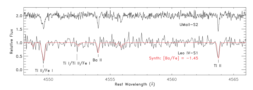
Figure 1.— Spectrum of Leo IV-S1 around the Ba II $\lambda 4554$ Å line. Despite the low S/N at these wavelengths, Ba is clearly detected. Lines of Ti and Fe are also marked. The red line is a synthetic spectrum from MOOG using the derived atmospheric parameters and abundance ratios, and the spectrum of UMaII-S2 ($T_{eff}=4600$ K, $\rm{[Fe/H]}=-3.23$) from Frebel et al. (2010a) is shown above for comparison.

Since the photometric and spectroscopic solutions for $T_{eff}$ and $\log{g}$ are not entirely consistent, assessing the impact that our choices for these parameters have on the derived abundances is important. An estimate of the systematic uncertainties can be obtained from the abundance differences between the two sets of stellar parameters. To quantify these further, we also vary the atmospheric parameters one at a time by approximately their uncertainties and examine the resulting abundance changes. The parameter uncertainties are set by considering how large a change is allowed by the Fe I abundances for $\xi$ and $T_{eff}$, and assigning reasonable uncertainty levels for the gravity and overall metallicity: $\Delta T_{eff}=+150$ K, $\Delta$log g $=-0.5$ dex, $\Delta\mbox{[M/H]}=+0.3$ dex, and $\Delta\xi=+0.3$ km s^-1. The systematic uncertainties we derive are listed in Tables 2 and 3. Over this range of parameters, the maximum iron abundance we obtain is $\rm{[Fe/H]}=-2.96$, so we can confidently conclude that Leo IV-S1 is indeed an EMP star.

4. DISCUSSION

4.1. The Frequency of EMP Stars in Dwarf Galaxies

Including Leo IV-S1, there are now detailed abundance studies (with individually determined atmospheric parameters) for ten stars in the ultra-faint dwarfs (Koch et al., 2008; Frebel et al., 2010a; Norris et al., 2009). The highest metallicity star included in these studies has $\rm{[Fe/H]}=-2.0$ (Koch et al., 2008), and four have metallicities below $\rm{[Fe/H]}=-3.0$. As noted by Frebel et al. (2010a), with the exception of Boo-1137 from Norris et al. (2009) these stars have been selected independent of their metallicities: the sole selection criterion (by necessity) is their apparent magnitude. The 33% success rate (3 out of 9, after excluding Boo-1137) at finding EMP stars strongly suggests that a substantial fraction of the stars in these systems have extremely low metallicities (Kirby et al., 2008; Salvadori & Ferrara, 2009). In order to obtain 3 EMP stars in a random drawing out of a sample of 9, the EMP fraction must be at least 10% at the 95% confidence level. The results of Norris et al. (2008) that 4 of 16 stars observed at medium resolution in Boo I (including Boo-1137) have metallicities below $\rm{[Fe/H]}=-3.0$ provides further support for this case. As the observed data sets increase further, it therefore seems likely that many more EMP stars, and perhaps stars with even lower metallicities, will be identified. Provided that one is willing to invest the telescope time to obtain high-resolution spectra of 18th-19th magnitude stars, the ultra-faint dwarfs may be the most promising targets for increasing samples of stars with $\rm{[Fe/H]}<-3.5$ and studying the fossil clues left behind by the first generation of stars.

4.2. Abundance Patterns in the Ultra-Faint Dwarfs

The abundances of light and iron-peak elements in Leo IV-S1 match closely those that we measured in UMa II and ComBer. The $\alpha$ elements Mg, Ca, and Ti are each enhanced by $\sim 0.3$ dex compared to the solar ratios, identical within the uncertainties to those of the two EMP stars in UMa II. Sc, Cr, and Ni in Leo IV-S1 also agree with the measured abundances of UMa II below $\rm{[Fe/H]}=-3$. Only a conservative [C/Fe] limit could be obtained for Leo IV-S1, indicating that the star is not strongly C-enriched. These similarities suggest that whatever process is responsible for producing elements from Na at least through the iron-peak in the ultra-faint dwarfs seems to be nearly universal, yielding similar abundances in almost every star examined so far. The only exception is the ratio of hydrostatic to explosive $\alpha$ elements (e.g., [Mg/Ca]), which is strongly enhanced in a fraction of the ultra-faint dwarf stars (Koch et al., 2008; Frebel et al., 2010a; Feltzing et al., 2009). As found by Frebel et al. (2010a) and illustrated in Fig. 2, this common abundance pattern in ultra-faint dwarf stars (including Leo IV-S1) also agrees well with that of EMP stars in the Milky Way halo (e.g., Cayrel et al., 2004; Lai et al., 2008).

Moreover, Leo IV-S1 continues the trend of unusually low neutron-capture abundances in the ultra-faint dwarfs (Koch et al., 2008; Frebel et al., 2010a), with $\rm{[Ba/Fe]}=-1.45$ and $\rm{[Sr/Fe]}=-1.02$. Unlike the lighter species, for heavy elements the ultra-faints as a whole do not agree with typical halo behavior; the halo has a higher mean abundance and spans a larger range of [nc/Fe] at similar metallicities (Fig. 2; also see François et al., 2007; Lai et al., 2008). Stars in the brighter dwarf spheroidals (dSphs) generally have roughly solar abundances of Ba and Eu, although a few of the most metal-poor stars in those galaxies show a similar deficiency of heavy elements as the ultra-faint dwarfs (Fulbright, Rich, & Castro, 2004; Frebel, Kirby, & Simon, 2010b). This distinction from both the halo and the classical dSphs suggests that the heavy elements may be produced differently in the ultra-faint dwarfs than in their brighter counterparts (at least at later times).

Abundance measurements of the few strongly r-process enhanced EMP stars in the halo indicate that SNe that produce r-process elements in large quantities must be rare (e.g., McWilliam et al., 1995b) or inefficient at dispersing those elements into the surrounding gas. It has been suggested that core-collapse SNe over a narrow mass range are the astrophysical site for the main r-process, perhaps in the lowest mass SNe ($8-10$ M_⊙) (e.g., Qian & Wasserburg, 2003; Wanajo et al., 2003). If the enrichment of all of the ultra-faint dwarfs is a result of randomly sampling supernovae from a common initial mass function (IMF), and assuming the main r-process to be the dominant source for the observed neutron-capture elements, then most dwarfs that incompletely sample the SN mass function will show deficient [Sr/Fe] and [Ba/Fe] ratios because r-process SNe are rare. A small fraction, however, should contain relatively r-process rich EMP stars. Since the IMF of the first stars is expected to be top-heavy (e.g., Yoshida et al., 2006), the low r-process abundances we observe could arise naturally if r-process elements are predominantly made by these lower-mass SNe.

Despite the overall broad similarities with the other ultra-faints, possible signs of stochasticity in the abundance patterns of the faintest dwarfs are also evident in the data that have been acquired over the past few years. Two stars in Hercules and one each in Boo I (Feltzing et al., 2009) and Draco (Fulbright et al., 2004) exhibit very high $\rm{[Mg/Ca]}$ ratios that are argued to result from small numbers of supernovae and the resulting incomplete sampling of the IMF (Koch et al., 2008). The Hercules stars also have extremely low (nearly unprecedented; see Fig. 2) upper limits for [Ba/Fe], while Ba has been detected in every star observed so far in UMa II, ComBer, and Leo IV, despite much lower overall metallicities. It may be noteworthy that it is the most luminous ultra-faint dwarfs that seem to contain these unusual signatures, but larger samples in all of these galaxies are needed before drawing strong conclusions.

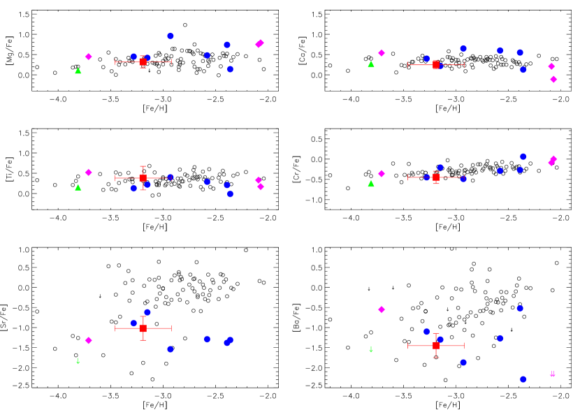
Figure 2.— Abundance pattern of Leo IV-S1 (filled red square) compared to stars in other ultra-faint dwarf galaxies (filled blue circles: ComBer and UMa II from Frebel et al. 2010a; filled magenta diamonds: Boötes I and Hercules from Koch et al. 2008 and Norris et al. 2009; filled green triangle: Sculptor star S1020549 from Frebel et al. 2010b) and a representative sample of metal-poor Milky Way halo stars (open black circles) from Cayrel et al. (2004), Cohen et al. (2004), Aoki et al. (2005), François et al. (2007), and Lai et al. (2008). With the possible exception of the two relatively metal-rich stars in Hercules at $\mbox{[Fe/H]}=-2$, the distribution of $\alpha$ and iron-peak abundance ratios is very similar across all of the ultra-faint dwarfs and the halo. All data displayed here have been adjusted to the Asplund et al. (2009) solar abundance scale.

4.3. Supernovae and Nucleosynthesis in Leo IV

Heger & Woosley (2008) have shown that Population III SNe from initially metal-free massive stars can produce an elemental abundance pattern similar to that measured by Cayrel et al. (2004) for EMP halo stars. In a similar study, Tominaga, Umeda, & Nomoto (2007) concluded that Pop III hypernovae with unusually high energies are necessary to match the Cayrel et al. (2004) data. The agreement between the abundances of Leo IV-S1 and the Cayrel et al. sample suggests that some form of Pop III nucleosynthesis may be able to explain the chemical abundances of Leo IV as well. In Fig. 3 we demonstrate the quality of the match that can be obtained between the observed abundances and the models; the best fit found by comparisons with the grid of models from Heger & Woosley (2008) is for a low-mass ($\sim 10$ M_⊙) SN with an average explosion energy. Higher mass hypernova explosions can also provide acceptable fits.

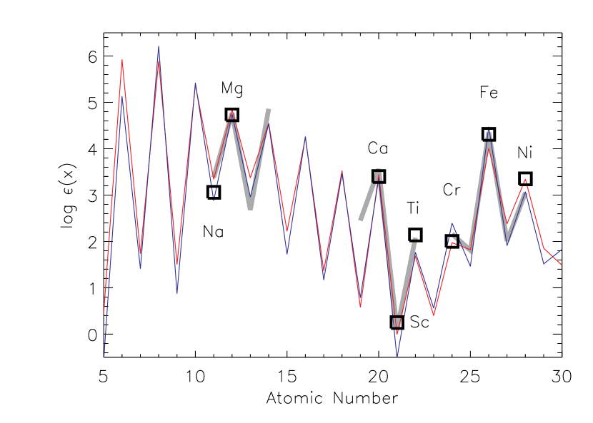
Figure 3.— Observed abundance pattern of Leo IV-S1 (black squares) compared to the Cayrel et al. (2004) halo sample (thick gray line) at similar metallicities and Population III supernova nucleosynthesis models from Heger & Woosley (2008). A Heger & Woosley “standard” 10.2 M_⊙ model (red line), diluted by $4700$ M_⊙ of primordial gas, reproduces the overall abundance pattern fairly well. A high explosion energy 29.5 M_⊙ Heger & Woosley SN (added to $2.6\times 10^{5}$ M_⊙ of hydrogen) predicts a similar pattern for many elements but with discrepant abundances for Sc and Cr (blue line).

Because the number of stars in Leo IV is so small ($L_{V}=14000$ L_⊙), the metal content of the entire galaxy is extremely low. For example, given the mean metallicity determined by Kirby et al. (2008) and assuming a stellar mass-to-light ratio of 1 M_⊙/L_⊙, Leo IV contains just 0.042 M_⊙ of Fe. Since this is comparable to the amount of Fe produced by the best-fitting Pop III SN models (Heger & Woosley, 2008), if Leo IV was indeed enriched by such explosions then a single supernova may be enough to have produced all of the observed heavy elements. It is also possible, of course, that multiple supernovae contributed to the chemical evolution of the galaxy if most of the metals were blown out via winds rather than having been incorporated into subsequent generations of stars. Nevertheless, we tentatively conclude that Leo IV-S1 may reflect the nucleosynthetic yields of the first Pop III star that the galaxy formed, at a time when its gas content was $\sim 4\times 10^{4}$ M_⊙. Other ultra-faint dwarfs therefore might reveal the abundance patterns of SNe with different masses, consistent with recent observations of Hercules (Koch et al., 2008)

5. SUMMARY AND CONCLUSIONS

We have carried out a high-resolution abundance analysis for the brightest star in the ultra-faint dwarf galaxy Leo IV. With $\rm{[Fe/H]}=-3.2$, Leo IV-S1 adds to the rapidly increasing sample of extremely metal-poor stars in dwarf galaxies. The low metallicity of Leo IV-S1 provides further support for the hypothesis that a substantial fraction ($\gtrsim 10$%) of the stars in the faintest dwarfs lie in the EMP regime.

The abundance pattern in Leo IV is extremely similar to that found in both the other ultra-faint dwarfs and the metal-poor Milky Way halo. As suggested by Frebel et al. (2010a), this excellent agreement demonstrates that the metal-poor end of the halo metallicity distribution could have been formed in galaxies like the ultra-faint dwarfs. The only exception to the close match between the halo and the ultra-faint dwarfs is the neutron-capture elements, which still appear somewhat lower in the dwarfs, but more measurements of these elements are needed.

Interestingly, the most metal-poor stars in some of the brighter dSphs seem to share the same chemical signature of $\alpha$-enhancement and neutron-capture depletion (Fulbright et al., 2004; Frebel et al., 2010b), although the abundances in those systems deviate substantially at higher metallicities (Shetrone et al., 2003; Venn et al., 2004). The similarity between the abundances of Leo IV-S1 and other dwarfs such as UMa II, ComBer, Boo I, and Sculptor suggests that the initial enrichment in many galaxies may have been universal. Differences between the abundances in the faintest dwarfs (ComBer, UMa II, and Leo IV) and the stars in somewhat more luminous systems, on the other hand, could point to stochastic chemical variations. Finally, we show that the abundance pattern of Leo IV-S1 is consistent with Population III supernova models, raising the possibility that Leo IV was enriched by some of the first stars.

Table 1 Equivalent width measurements

Element	$\lambda$	$\chi$	$\log{gf}$	EW	$\log{\epsilon}$
	[Å]	[eV]		[mÅ]
Na I	5889.973	0.00	+0.100	220.0	+3.28
Na I	5895.940	0.00	$-$0.200	160.0	+2.84
Mg I	4571.102	0.00	$-$5.670	64.0	+4.47
Mg I	4703.003	4.34	$-$0.520	75.0	+5.11
Mg I	5172.698	2.71	$-$0.380	231.0	+4.66
Mg I	5183.619	2.72	$-$0.160	256.0	+4.66
Mg I	5528.418	4.34	$-$0.341	74.0	+4.76
Ca I	5588.764	2.52	+0.358	47.0	+3.39
Ca I	5594.471	2.52	+0.097	22.0	+3.22
Ca I	6102.727	1.88	$-$0.770	38.0	+3.51
Ca I	6122.226	1.89	$-$0.320	62.0	+3.38
Ca I	6162.180	1.90	$-$0.090	90.0	+3.47
Ca I	6439.083	2.52	+0.390	61.0	+3.45
Sc II	5031.024	1.36	$-$0.400	41.0	+0.27
Sc II	5526.821	1.77	+0.020	42.0	+0.33
Sc II	5657.880	1.51	$-$0.600	18.0	+0.14
Ti I	5039.964	0.02	$-$1.130	25.0	+1.76
Ti I	5210.392	0.05	$-$0.884	58.0	+2.01
Ti II	4417.723	1.16	$-$1.430	82.0	+2.13
Ti II	4443.812	1.08	$-$0.700	127.0	+1.95
Ti II	4468.500	1.13	$-$0.600	120.0	+1.79
Ti II	4501.278	1.12	$-$0.750	136.0	+2.15
Ti II	4563.766	1.22	$-$0.960	122.0	+2.24
Ti II	4571.982	1.57	$-$0.530	111.0	+2.12
Ti II	4589.953	1.24	$-$1.790	70.0	+2.37
Ti II	5185.908	1.89	$-$1.350	26.0	+2.02
Ti II	5336.794	1.58	$-$1.700	63.0	+2.48
Ti II	5381.028	1.57	$-$2.080	21.0	+2.19
Cr I	4254.346	0.00	$-$0.114	141.0	+1.92
Cr I	5345.807	1.00	$-$0.980	26.0	+2.08
Fe I	4447.728	2.22	$-$1.339	77.0	+4.30
Fe I	4494.573	2.20	$-$1.136	74.0	+4.01
Fe I	4871.325	2.86	$-$0.362	60.0	+3.81
Fe I	4872.144	2.88	$-$0.567	91.0	+4.44
Fe I	4890.763	2.87	$-$0.394	71.0	+3.99
Fe I	4891.502	2.85	$-$0.111	83.0	+3.83
Fe I	4994.138	0.91	$-$2.956	71.0	+3.93
Fe I	5041.076	0.96	$-$3.086	86.0	+4.29
Fe I	5041.763	1.48	$-$2.203	114.0	+4.46
Fe I	5049.827	2.28	$-$1.355	67.0	+4.09
Fe I	5123.730	1.01	$-$3.058	115.0	+4.66
Fe I	5127.368	0.91	$-$3.249	81.0	+4.31
Fe I	5133.699	4.18	+0.140	23.0	+4.38
Fe I	5150.852	0.99	$-$3.037	113.0	+4.58
Fe I	5151.917	1.01	$-$3.321	70.0	+4.38
Fe I	5166.284	0.00	$-$4.123	94.0	+4.08
Fe I	5171.610	1.48	$-$1.721	118.0	+3.98
Fe I	5191.465	3.04	$-$0.551	47.0	+4.01
Fe I	5192.353	3.00	$-$0.421	83.0	+4.27
Fe I	5194.949	1.56	$-$2.021	120.0	+4.41
Fe I	5216.283	1.61	$-$2.082	91.0	+4.17
Fe I	5225.534	0.11	$-$4.755	82.0	+4.72
Fe I	5232.952	2.94	$-$0.057	109.0	+4.13
Fe I	5250.216	0.12	$-$4.938	68.0	+4.76
Fe I	5281.798	3.04	$-$0.833	48.0	+4.29
Fe I	5283.629	3.24	$-$0.524	40.0	+4.13
Fe I	5302.307	3.28	$-$0.720	55.0	+4.57
Fe I	5307.369	1.61	$-$2.912	48.0	+4.48
Fe I	5324.191	3.21	$-$0.103	99.0	+4.39
Fe I	5497.526	1.01	$-$2.825	128.0	+4.49
Fe I	5501.477	0.96	$-$3.046	110.0	+4.41
Fe I	5506.791	0.99	$-$2.789	142.0	+4.60
Fe I	5569.631	3.42	$-$0.500	54.0	+4.49
Fe I	5572.851	3.40	$-$0.275	57.0	+4.27
Fe I	5615.658	3.33	+0.050	82.0	+4.14
Fe I	6136.624	2.45	$-$1.410	82.0	+4.37
Fe I	6137.702	2.59	$-$1.346	66.0	+4.32
Fe I	6191.571	2.43	$-$1.416	95.0	+4.48
Fe I	6219.287	2.20	$-$2.448	40.0	+4.58
Fe I	6230.736	2.56	$-$1.276	60.0	+4.13
Fe I	6252.565	2.40	$-$1.767	59.0	+4.39
Fe I	6265.141	2.18	$-$2.550	21.0	+4.31
Fe I	6335.337	2.20	$-$2.180	43.0	+4.34
Fe I	6393.612	2.43	$-$1.576	68.0	+4.33
Fe I	6400.009	3.60	$-$0.290	40.0	+4.24
Fe I	6411.658	3.65	$-$0.595	25.0	+4.35
Fe I	6421.360	2.28	$-$2.014	44.0	+4.28
Fe I	6430.856	2.18	$-$1.946	75.0	+4.44
Fe I	6494.994	2.40	$-$1.239	100.0	+4.28
Fe I	6677.997	2.69	$-$1.420	58.0	+4.38
Fe I	6750.164	2.42	$-$2.621	13.0	+4.43
Fe II	4923.930	2.89	$-$1.260	84.0	+4.02
Fe II	5018.450	2.89	$-$1.110	120.0	+4.35
Fe II	5197.560	3.23	$-$2.220	44.0	+4.83
Fe II	5276.000	3.20	$-$2.010	67.0	+4.88
Fe II	6456.391	3.90	$-$2.075	21.0	+5.00
Ni I	6643.638	1.68	$-$2.300	48.0	+3.56
Ni I	6767.784	1.83	$-$2.170	20.0	+3.15
Sr II	4215.539	0.00	$-$0.170	120.0	$-$1.34
Ba II	4554.036	0.00	+0.160	62.0	$-$2.46

Table 2Stellar Parameters and Abundances for Leo IV-S1

	Fiducial Model					Spectroscopic Model
	$\overline{\phantom{string}}$					$\overline{\phantom{string}}$
Parameter/	Value/	$\log{\epsilon(X)}$	N${}_{\mbox{lines}}$	$\sigma_{\mbox{stat}}$	$\sigma_{\mbox{sys}}$	Value/
Species	Abundance Ratio					Abundance Ratio
$M_{r}$	$-2.18$.					$-2.18$.
$T_{eff}$ [K]	04330.					04200.
$\log{g}$	001.00					000.00
$\xi$ [km s-1]	003.20					003.20
$\rm{[Fe~{}I/H]}$	$-3.19$.	4.31	50	0.03	0.27	$-3.09$.
$\rm{[Fe~{}II/H]}$	$-2.88$:	4.62:	5	0.19	0.14	$-2.89$:
$\rm{[C/Fe]}$	$<$$-0.08$+.	$<$ 5.16	synth	…	…	$<0.32$0.
$\rm{[Na~{}I/Fe]}$	+0.01.	3.06	2	0.28	0.09	$-0.04$.
$\rm{[Mg~{}I/Fe]}$	+0.32.	4.73	5	0.12	0.09	+0.62.
$\rm{[Ca~{}I/Fe]}$	+0.25.	3.40	6	0.05	0.09	+0.26.
$\rm{[Ti~{}I/Fe]}$	+0.13.	1.89	2	0.16	0.07	+0.08.
$\rm{[Ti~{}II/Fe]}$	+0.38.	2.14	10	0.06	0.28	+0.40.
$\rm{[Sc~{}II/Fe]}$	+0.29.	0.25	3	0.06	0.33	+0.00.
$\rm{[Cr~{}I/Fe]}$	$-0.45$.	2.00	2	0.10	0.11	$-0.44$.
$\rm{[Ni~{}I/Fe]}$	+0.32.	3.35	2	0.26	0.07	+0.16.
$\rm{[Sr~{}II/Fe]}$	$-1.02$.	$-1.34$	1	…	0.26	$-0.96$.
$\rm{[Ba~{}II/Fe]}$	$-1.45$.	$-2.46$	1	…	0.24	$-1.56$.

Note. — All abundance ratios [X/Fe] (including ionized species) are calculated relative to Fe I.

Table 3Abundance Uncertainties

Species	$\Delta\log{\epsilon(X)}$	$\Delta\log{\epsilon(X)}$	$\Delta\log{\epsilon(X)}$	$\Delta\log{\epsilon(X)}$
	for $T_{eff}+150$ K	for $\log{g}-0.5$ dex	for $\mbox{[M/H]}+0.3$	for $\xi+0.3$ km s-1
Fe I	+0.23	+0.13	$-0.03$	$-0.04$
Fe II	$-0.08$	$-0.10$	+0.01	$-0.05$
Na I	+0.24	+0.14	$-0.07$	$-0.12$
Mg I	+0.19	+0.21	$-0.05$	$-0.06$
Ca I	+0.15	+0.10	$-0.02$	$-0.01$
Ti I	+0.29	+0.14	$-0.04$	$-0.01$
Ti II	$-0.01$	+0.00	+0.01	$-0.06$
Sc II	+0.02	$-0.12$	+0.02	$-0.01$
Cr I	+0.25	+0.21	$-0.09$	$-0.07$
Ni I	+0.25	+0.07	$-0.01$	$-0.01$
Sr II	$-0.01$	+0.07	$-0.04$	$-0.11$
Ba II	+0.07	$-0.04$	+0.02	$-0.02$

References

- Adelman-McCarthy et al. (2007) Adelman-McCarthy, J. K., et al. 2007, ApJS, 172, 634
- Alonso et al. (1999) Alonso, A., Arribas, S., & Martínez-Roger, C. 1999, A&AS, 140, 261
- Aoki et al. (2005) Aoki, W., et al. 2005, ApJ, 632, 611
- Aoki et al. (2009) Aoki, W., et al. 2009, A&A, 502, 569
- Asplund et al. (2009) Asplund, M., Grevesse, N., Sauval, A. J., & Scott, P. 2009, ARA&A, 47, 481
- Belokurov et al. (2007) Belokurov, V., et al. 2007, ApJ, 654, 897
- Bernstein et al. (2003) Bernstein, R., Shectman, S. A., Gunnels, S. M., Mochnacki, S., & Athey, A. E. 2003, Proc. SPIE, 4841, 1694
- Bovill & Ricotti (2009) Bovill, M. S., & Ricotti, M. 2009, ApJ, 693, 1859
- Cayrel et al. (2004) Cayrel, R., et al. 2004, A&A, 416, 1117
- Cohen et al. (2004) Cohen, J. G., et al. 2004, ApJ, 612, 1107
- Cohen & Huang (2009) Cohen, J. G., & Huang, W. 2009, ApJ, 701, 1053
- de Jong et al. (2010) de Jong, J. T. A., Martin, N. F., Rix, H.-W., Smith, K. W., Jin, S., & Macció, A. V. 2010, ApJ, 710, 1664
- Feltzing et al. (2009) Feltzing, S., Eriksson, K., Kleyna, J., & Wilkinson, M. I. 2009, A&A, 508, L1
- François et al. (2007) François, P., et al. 2007, A&A, 476, 935
- Frebel et al. (2010a) Frebel, A., Simon, J. D., Geha, M., & Willman, B. 2010a, ApJ, 708, 560
- Frebel et al. (2010b) Frebel, A., Kirby, E. N., & Simon, J. D., 2010b, Nature, 464, 72
- Fulbright et al. (2004) Fulbright, J. P., Rich, R. M., & Castro, S. 2004, ApJ, 612, 447
- Girardi et al. (2004) Girardi, L., Grebel, E. K., Odenkirchen, M., & Chiosi, C. 2004, A&A, 422, 205
- Heger & Woosley (2008) Heger, A., & Woosley, S. E. 2008, submitted to ApJ (preprint at arXiv:0803.3161)
- Helmi et al. (2006) Helmi, A., et al. 2006, ApJ, 651, L121
- Jordi et al. (2006) Jordi, K., Grebel, E. K., & Ammon, K. 2006, A&A, 460, 339
- Kelson (2003) Kelson, D. D. 2003, PASP, 115, 688
- Kirby et al. (2008) Kirby, E. N., Simon, J. D., Geha, M., Guhathakurta, P., & Frebel, A. 2008, ApJ, 685, L43
- Koch et al. (2008) Koch, A., McWilliam, A., Grebel, E. K., Zucker, D. B., & Belokurov, V. 2008, ApJ, 688, L13
- Koch et al. (2009) Koch, A., Côté, P., & McWilliam, A. 2009, A&A, 506, 729
- Kurucz (1992) Kurucz, R. L. 1992, The Stellar Populations of Galaxies, 149, 225
- Lai et al. (2008) Lai, D. K., Bolte, M., Johnson, J. A., Lucatello, S., Heger, A., & Woosley, S. E. 2008, ApJ, 681, 1524
- Martin et al. (2008) Martin, N. F., de Jong, J. T. A., & Rix, H.-W. 2008, ApJ, 684, 1075
- McWilliam et al. (1995a) McWilliam, A., Preston, G. W., Sneden, C., & Shectman, S. 1995a, AJ, 109, 2736
- McWilliam et al. (1995b) McWilliam, A., Preston, G. W., Sneden, C., & Searle, L. 1995b, AJ, 109, 2757
- Moretti et al. (2009) Moretti, M. I., et al. 2009, ApJ, 699, L125
- Norris et al. (2008) Norris, J. E., Gilmore, G., Wyse, R. F. G., Wilkinson, M. I., Belokurov, V., Evans, N. W., & Zucker, D. B. 2008, ApJ, 689, L113
- Norris et al. (2009) Norris, J. E., Yong, D., Gilmore, G., & Wyse, R. F. G. 2010, ApJ, 711, 350
- Qian & Wasserburg (2003) Qian, Y.-Z., & Wasserburg, G. J. 2003, ApJ, 588, 1099
- Salvadori & Ferrara (2009) Salvadori, S., & Ferrara, A. 2009, MNRAS, 395, L6
- Sand et al. (2009) Sand, D. J., Seth, A., Olszewski, E. W., Willman, B., Zaritsky, D., & Kallivayalil, N. 2009, submitted to ApJ (preprint at arXiv:0911.5352)
- Schlegel et al. (1998) Schlegel, D. J., Finkbeiner, D. P., & Davis, M. 1998, ApJ, 500, 525
- Shetrone et al. (2003) Shetrone, M., Venn, K. A., Tolstoy, E., Primas, F., Hill, V., & Kaufer, A. 2003, AJ, 125, 684
- Simon & Geha (2007) Simon, J. D., & Geha, M. 2007, ApJ, 670, 313 (SG07)
- Sneden (1973) Sneden, C. 1973, ApJ, 184, 839
- Tominaga et al. (2007) Tominaga, N., Umeda, H., & Nomoto, K. 2007, ApJ, 660, 516
- Venn et al. (2004) Venn, K. A., Irwin, M., Shetrone, M. D., Tout, C. A., Hill, V., & Tolstoy, E. 2004, AJ, 128, 1177
- Wanajo et al. (2003) Wanajo, S., Tamamura, M., Itoh, N., Nomoto, K., Ishimaru, Y., Beers, T. C., & Nozawa, S. 2003, ApJ, 593, 968
- Yoshida et al. (2006) Yoshida, N., Omukai, K., Hernquist, L., & Abel, T. 2006, ApJ, 652, 6