Structure Formation by the Fifth Force: Segregation of Baryons and Dark Matter

Abstract

In this paper we present the results of $N$-body simulations with a scalar field coupled differently to cold dark matter (CDM) and baryons. The scalar field potential and coupling function are chosen such that the scalar field acquires a heavy mass in regions with high CDM density and thus behaves like a chameleon. We focus on how the existence of the scalar field affects the formation of nonlinear large-scale structure, and how the different couplings of the scalar field to baryons and CDM particles lead to different distributions and evolutions for these two matter species, both on large scales and inside virialized halos. As expected, the baryon-CDM segregation increases in regions where the fifth force is strong, and little segregation in dense regions. We also introduce an approximation method to identify the virialized halos in coupled scalar field models which takes into account the scalar field coupling and which is easy to implement numerically. It is find that the chameleon nature of the scalar field makes the internal density profiles of halos dependent on the environment in a very nontrivial way.

I Introduction

The origin and nature of the dark energy Copeland (2006) is one of the most difficult challenges facing physicists and cosmologists now. Among all the proposed models to tackle this problem, a scalar field is perhaps the most popular one up to now. The scalar field, denoted by $\varphi$, might only interact with other matter species through gravity, or have a coupling to normal matter and therefore producing a fifth force on matter particles. This latter idea has seen a lot of interests in recent years, in the light that such a coupling could potentially alleviate the coincidence problem of dark energy Amendola (2000) and that it is commonly predicted by low energy effective theories from a fundamental theory.

Nevertheless, if there is a coupling between the scalar field and baryonic particles, then stringent experimental constraints might be placed on the fifth force on the latter provided that the scalar field mass is very light (which is needed for the dark energy). Such constraints severely limit the viable parameter space of the model. Different ways out of the problem have been proposed, of which the simplest one is to have the scalar field coupling to dark matter only but not to standard model particles, therefore evading those constraints entirely. This is certainly possible, especially because both dark matter and dark energy are unknown to us and they may well have a common origin. Another interesting possibility is to have the chameleon mechanism Khoury (2004, 2004); Mota (2006, 2006), by virtue of which the scalar field acquires a large mass in high density regions and thus the fifth force becomes undetectablly short-ranged, and so also evades the constraints.

Study of the cosmological effect of a chameleon scalar field shows that the fifth force is so short-ranged that it has negligible effect in the large scale structure formation Brax (2004) for certain choices of the scalar field potential. But it is possible that the scalar field has a large enough mass in the solar system to pass any constraints, and at the same time has a low enough mass (thus long range forces) on cosmological scales, producing interesting phenomenon in the structure formation. This is the case of some $f(R)$ gravity models Carroll (2004); Nojiri (2003), which survives solar system tests thanks again to the chameleon effect Navarro (2007); Li (2007); Hu (2007); Brax (2008). Note that the $f(R)$ gravity model is mathematically equivalent to a scalar field model with matter coupling.

No matter whether the scalar field couples with dark matter only or with all matter species, it is of general interests to study its effects in cosmology, especially in the large scale structure formation. Indeed, at the linear perturbation level there have been a lot of studies about the coupled scalar field and $f(R)$ gravity models which enable us to have a much clearer picture about their behaviors now. But linear perturbation studies do not conclude the whole story, because it is well known that the matter distribution at late times becomes nonlinear, making the behavior of the scalar field more complex and the linear analysis insufficient to produce accurate results to confront with observations. For the latter purpose the best way is to perform full $N$-body simulations Bertschinger (1998) to evolve the individual particles step by step.

$N$-body simulations for scalar field and relevant models have been performed before Linder (2003); Mainini (2003); Springel (2007); Kesden (2006); Farrar (2007); Keselman (2009); Maccio (2004); Baldi (2008). For example, in Maccio (2004) the simulation is about a specific coupled scalar field model. This study however does not obtain a full solution to the spatial configuration of the scalar field, but instead simplifies the simulation by assuming that the scalar field’s effect is to change the value of the gravitational constant, and presenting an justifying argument for such an approximation. As discussed in Li (2009); Zhao (2009), this approximation is only good in certain parameter spaces and for certain choices of the scalar field potential, and therefore full simulations tare needed to study the scalar field behaviour more rigorously.

Recently there have also appeared $N$-body simulations of the $f(R)$ gravity model Oyaizu (2008, 2008), which do solve the scalar degree of freedom explicitly. However, embedded in the $f(R)$ framework there are some limitations in the generality of these works. As a first thing, $f(R)$ gravity model (no matter what the form $f$ is) only corresponds to the couple scalar field models for a specific value of coupling strength Amendola (2007). Second, in $f(R)$ models the correction to standard general relativity is through the modification to the Poisson equation and thus to the gravitational potential as a whole Oyaizu (2008), while in the coupled scalar field models we could clearly separate the scalar fifth force from gravity and analyze the former directly Li (2009). Also, in $f(R)$ models, as well as the scalar-tensor theories, the coupling between matter and the scalar field is universal (the same to dark matter and baryons), while in the couple scalar field models it is straightforward to switch on/off the coupling to baryons and study the effects on baryonic and dark matter clusterings respectively (as we will do in this paper). Correspondingly, the general framework of $N$-body simulations in coupled scalar field models could also handle the situation where the chameleon effect is absent and/or scalar field only couples to dark matter, and thus provide a testbed for possible violations of the weak equivalence principle.

In this paper we shall go beyond Li (2009) and consider the case where the chameleon scalar field couples differently to different species of matter. To be explicit, we consider two matter species, and let one of them have no coupling to the scalar field. Because it is commonly believed that normal baryons, being observable in a variety of experiments, should have extremely weak (if any) coupling to scalar fields, we call the uncoupled matter species in our simulation ”baryons”. It is however reminded here that this matter species is not really baryonic in the sense that it does not experience normal baryonic interactions. The inclusion of true baryons will make the investigation more complicated and is thus beyond the scope of the present work.

The paper is organized as follows: in § II we list the essential equations to be implemented in the $N$-body simulations and describe briefly the difference from normal LCDM simulations. § III is the main body of the paper, in which § III.1 gives the details about our simulations, such as code description and parameter set-up, § III.2 displays some preliminary results for visualization, such as baryon/CDM distribution, potential/scalar field configuration and the correlation between the fifth force (for CDM particles) and gravity; § III.3 quantifies the nonlinear matter power spectrum of our model, especially the difference from LCDM results and the bias between CDM and baryons; § III.4 briefly describes the essential modifications one must bear in mind when identifying virialized halos from the simulation outputs and shows the mass functions for our models; § III.5 we pick out two halos from our simulation box and analyzes their total internal profiles, as well as their baryonic/CDM density profiles. We finally summarize in § IV.

II The Equations

In this section we first describe the method to simulate structure formation with two differently coupled matter species and the appropriate equations to be used. Those equations for a single matter species have been discussed in details previously in Li (2009), but the inclusion of different matter species requires further modifications and we list all these for completeness.

II.1 The Fundamental Equations

The Lagrangian for our coupled scalar field model is

$$\mathcal{L} = \frac{1}{2}\left[\frac{R}{\kappa}-\nabla^{a}\varphi\nabla_{a}\varphi\right]+V(\varphi)-C(\varphi)\mathcal{L}_{\mathrm{CDM}}+\mathcal{L}_{\mathrm{S}}\ \$$ (1)

where $R$ is the Ricci scalar, $\kappa=8\pi G$ with $G$ Newton’s constant, $\varphi$ is the scalar field, $V(\varphi)$ is its potential energy and $C(\varphi)$ its coupling to dark matter, which is assumed to be cold and described by the Lagrangian $\mathcal{L}_{\mathrm{CDM}}$. $\mathcal{L}_{\mathrm{S}}$ includes all other matter species, in particular our baryons. The contribution from photons and neutrinos in the $N$-body simulations (for late times, i.e., $z\sim\mathcal{O}(1)$) is negligible, but should be included when generating the matter power spectrum from which the initial conditions for our $N$-body simulations are obtained (see below).

The dark matter Lagrangian for a point-like particle with bare mass $m_{0}$ is

$$\mathcal{L}_{\mathrm{CDM}}(\mathbf{y}) = -\frac{m_{0}}{\sqrt{-g}}\delta(\mathbf{y}-\mathbf{x}_{0})\sqrt{g_{ab}\dot{x}^{a}_{0}\dot{x}^{b}_{0}}$$ (2)

where $\mathbf{y}$ is the coordinate and $\mathbf{x}_{0}$ is the coordinate of the centre of the particle. From this equation it can be easily derived that

$$T^{ab}_{\mathrm{CDM}} = \frac{m_{0}}{\sqrt{-g}}\delta(\mathbf{y}-\mathbf{x}_{0})\dot{x}^{a}_{0}\dot{x}^{b}_{0}.$$ (3)

Also, because $g_{ab}\dot{x}^{a}_{0}\dot{x}^{b}_{0}\equiv g_{ab}u^{a}u^{b}=1$ where $u^{a}$ is the four velocity of the dark matter particle, the Lagrangian could be rewritten as

$$\mathcal{L}_{\mathrm{CDM}}(\mathbf{y}) = -\frac{m_{0}}{\sqrt{-g}}\delta(\mathbf{y}-\mathbf{x}_{0}),$$ (4)

which will be used below.

Eq. (3) is just the energy momentum tensor for a single dark matter particle. For a fluid with many particles the energy momentum tensor will be

$$T^{ab}_{\mathrm{CDM}} = \frac{1}{V}\int_{V}d^{4}y\sqrt{-g}\frac{m_{0}}{\sqrt{-g}}\delta(y-x_{0})\dot{x}^{a}_{0}\dot{x}^{b}_{0}$$ (5)

$$= \rho_{\mathrm{CDM}}u^{a}u^{b},$$

in which $V$ is a volume microscopically large and macroscopically small, and we have extended the 3-dimensional $\delta$ function to a 4-dimensional one by adding a time component. Here $u^{a}$ is the averaged 4-velocity of the collection of particles inside this volume, and is not necessarily the same as the $4$-velocity of the observer.

Meanwhile, using

$$T^{ab} = -\frac{2}{\sqrt{-g}}\frac{\delta\left(\sqrt{-g}\mathcal{L}\right)}{\delta g_{ab}}$$ (6)

it is straightforward to show that the energy momentum tensor for the scalar field is given by

$$T^{\varphi ab} = \nabla^{a}\varphi\nabla^{b}\varphi-g^{ab}\left[\frac{1}{2}\nabla_{c}\varphi\nabla^{c}\varphi-V(\varphi)\right].$$ (7)

So the total energy momentum tensor is

$$T_{ab} = \nabla_{a}\varphi\nabla_{b}\varphi-g_{ab}\left[\frac{1}{2}\nabla_{c}\varphi\nabla^{c}\varphi-V(\varphi)\right]$$ (8)

$$+C(\varphi)T^{\mathrm{CDM}}_{ab}+T^{\mathrm{S}}_{ab}$$

where $T^{\mathrm{CDM}}_{ab}=\rho_{\mathrm{CDM}}u_{a}u_{b}$, $T^{\mathrm{S}}_{ab}$ is the energy momentum tensor for all other matter species including baryons, and the Einstein equation is

$$G_{ab} = \kappa T_{ab}$$ (9)

where $G_{ab}$ is the Einstein tensor. Note that due to the coupling between the scalar field $\varphi$ and the dark matter, the energy momentum tensors for either will not be conserved, and we have

$$\nabla_{b}T^{\mathrm{CDM}ab} = -\frac{C_{\varphi}(\varphi)}{C(\varphi)}\left(g^{ab}\mathcal{L}_{\mathrm{CDM}}+T^{\mathrm{CDM}ab}\right)\nabla_{b}\varphi\ \$$ (10)

where throughout this paper we shall use a _φ to denote the derivative with respect to $\varphi$.

Finally, the scalar field equation of motion (EOM) from the given Lagrangian is

$$\square\varphi+\frac{\partial V(\varphi)}{\partial\varphi} = \frac{\partial C(\varphi)}{\partial\varphi}\mathcal{L}_{\mathrm{CDM}}$$

where $\square=\nabla^{a}\nabla_{a}$. Using Eq. (4) it can be rewritten as

$$\square\varphi+\frac{\partial V(\varphi)}{\partial\varphi}+\rho_{\mathrm{CDM}}\frac{\partial C(\varphi)}{\partial\varphi} = 0.$$ (11)

Eqs. (8, 9, 10, 11) summarize all the physics that will be used in our analysis.

We will consider a special form for the scalar field potential,

$$V(\varphi) = \frac{V_{0}}{\left[1-\exp\left(\beta\sqrt{\kappa}\varphi\right)\right]^{\mu}},$$ (12)

where $\mu$ and $\beta$ are dimensionless constants while $V_{0}$ has mass dimension four. As has been discussed in Li (2009), $\mu\ll 1$ to evade observational constraints and $\beta$ can be set to $-1$ without loss of generality, since we can always rescale $\varphi$ as we wish. Meanwhile, the coupling between the scalar field and dark matter particle is chosen as

$$C(\varphi) = \exp(\gamma\sqrt{\kappa}\varphi),$$ (13)

where $\gamma>0$ is yet another dimensionless constant characterizing the strength of the coupling.

As discussed in Li (2009), the two dimensionless parameters $\mu$ and $\gamma$ have clear physical meanings: roughly speaking, $\mu$ controls the time when the scalar field becomes important in cosmology while $\gamma$ determines how important the scalar field would ultimately be. In fact, the potential given in Eq. (12) is partly motivated by the $f(R)$ cosmology Li (2007), in which the extra degree of freedom behaves as a coupled scalar field in the Einstein frame. As we can see from Eq. (12), the potential $V\rightarrow\infty$ when $\varphi\rightarrow 0$ while $V\rightarrow V_{0}$ when $\varphi\rightarrow\infty$. In the latter case, however, $C\rightarrow\infty$, so that the effective total potential

$$V_{eff}(\varphi) = V(\varphi)+\rho_{\mathrm{CDM}}C(\varphi)$$ (14)

has a global minimum at some finite $\varphi$. If the total potential $V_{eff}(\varphi)$ is steep enough around this minimum, then the scalar field becomes very heavy and thus follows its minimum dynamically, as is in the case of the chameleon cosmology (see e.g. Brax (2004)). If $V_{eff}$ is not steep enough at the minimum, however, the scalar field will experience a more complicated evolution. These two different cases can be obtained by choosing appropriate values of $\gamma$ and $\mu$: if $\gamma$ is very large or $\mu$ is small then we run into the former situation and if $\gamma$ is small and $\mu$ is large we have the second. In reality, the situation can get even more complicated because when $\gamma$, which characterizes the coupling strength, increases, the CDM evolution could also get severely affected, which in turn has back-reactions on the scalar field itself.

II.2 Nonrelativistic Limit

The $N$-body simulation only probes the motion of particles at late times, and we are not interested in extreme conditions such as black hole formation/evolution, which mean that taking the non-relativistic limit of the above equations should be a sufficient approximation for our purpose.

The existence of the scalar field and its (different) couplings to matter particles lead to the following changes to the $\Lambda$CDM model: Firstly, the energy momentum tensor has a new piece of contribution from the scalar field; secondly, the energy density of dark matter in gravitational field equations is multiplied by the function $C(\varphi)$, which is because the coupling to scalar field essentially renormalizes the mass of dark matter particles; thirdly, dark matter particles will not follow geodesics in their motions as in $\Lambda$CDM, but rather the total force on them has a contribution, the fifth force, from the exchange of scalar field quanta; finally, CDM particles must be distinguished from baryons so that the fifth force only acts on the former and these two species only interact gravitationally. This last point is one main difference between the present work and a previous one Li (2009).

These imply that the following things need to be modified or added:

1. The scalar field $\varphi$ equation of motion, which determines the value of the scalar field at any given time and position;

2. The Poisson equation, which determines the gravitational potential (and thus gravity) at any given time and position, according to the local energy density and pressure, which include the contribution from the scalar field (as obtained from $\varphi$ equation of motion);

3. The total force on the dark matter particles, which is determined by the spatial configuration of $\varphi$, just like gravity is determined by the spatial configuration of the gravitational potential;

4. The CDM and baryonic particles must be tagged respectively so that the code knows to assign forces correctly to different species.

We shall describe these one by one now.

For the scalar field equation of motion, we denote $\bar{\varphi}$ as the background value of $\varphi$ and $\delta\varphi\equiv\varphi-\bar{\varphi}$ as the scalar field perturbation. Then Eq. (11) could be rewritten as

$$\ddot{\delta\varphi}+3H\dot{\delta\varphi}+\vec{\nabla}_{\mathbf{r}}^{2}\varphi+V_{,\varphi}(\varphi)-V_{,\varphi}(\bar{\varphi})$$

$$+\rho_{\mathrm{CDM}}C_{,\varphi}(\varphi)-\bar{\rho}_{\mathrm{CDM}}C_{,\varphi}(\bar{\varphi}) = 0$$

by subtracting the corresponding background equation from it. Here $\vec{\nabla}_{\mathbf{r}a}$ is the covariant spatial derivative with respect to the physical coordinate $\mathbf{r}=a\mathbf{x}$ with $\mathbf{x}$ the conformal coordinate, and $\vec{\nabla}^{2}_{\mathbf{r}}=\vec{\nabla}_{\mathbf{r}a}\vec{\nabla}_{\mathbf{r}}^{a}$. $\vec{\nabla}_{\mathbf{r}a}$ is essentially the $\hat{\nabla}_{a}$, but because here we are working in the weak field limit we approximate it as $\vec{\nabla}_{\mathbf{r}}^{2}=-\left(\partial^{2}_{r_{x}}+\partial^{2}_{r_{y}}+\partial^{2}_{r_{z}}\right)$ by assuming a flat background; the minus sign is because our metric convention is $(+,-,-,-)$ instead of $(-,+,+,+)$. For the simulation here we will also work in the quasi-static limit, assuming that the spatial gradient is much larger than the time derivative, $|\vec{\nabla}_{\mathbf{r}}\varphi|\gg|\frac{\partial\varphi}{\partial t}|$ (which will be justified below). Thus the above equation can be further simplified as

$$c^{2}\partial_{\mathbf{x}}^{2}(a\delta\varphi)$$

$$= a^{3}\left[V_{,\varphi}(\varphi)-V_{,\varphi}(\bar{\varphi})+\rho_{\mathrm{CDM}}C_{,\varphi}(\varphi)-\bar{\rho}_{\mathrm{CDM}}C_{,\varphi}(\bar{\varphi})\right],$$

in which $\partial^{2}_{\mathbf{x}}=-\vec{\nabla}_{\mathbf{x}}^{2}=+\left(\partial^{2}_{x}+\partial^{2}_{y}+\partial^{2}_{z}\right)$ is with respect to the conformal coordinate $\mathbf{x}$ so that $\vec{\nabla}_{\mathbf{x}}=a\vec{\nabla}_{\mathbf{r}}$, and we have restored the factor $c^{2}$ in front of $\vec{\nabla}_{\mathbf{x}}^{2}$ (the $\varphi$ here and in the remaining of this paper is $c^{-2}$ times the $\varphi$ in the original Lagrangian unless otherwise stated). Note that here $V$ and $\rho_{\mathrm{CDM}}$ both have the dimension of mass density rather than energy density.

Next look at the Poisson equation, which is obtained from the Einstein equation in weak-field and slow-motion limits. Here the metric could be written as

$$ds^{2} = (1+2\phi)dt^{2}-(1-2\psi)\delta_{ij}dr^{i}dr^{j}$$ (16)

from which we find that the time-time component of the Ricci curvature tensor $R^{0}_{\ 0}=-\vec{\nabla}_{\mathbf{r}}^{2}\phi$, and then the Einstein equation $R_{ab}=\kappa\left(T_{ab}-\frac{1}{2}g_{ab}T\right)$ gives

$$R^{0}_{\ 0}\ =\ -\vec{\nabla}_{\mathbf{r}}^{2}\phi\ =\ \frac{\kappa}{2}(\rho_{\mathrm{TOT}}+3p_{\mathrm{TOT}})$$ (17)

where $\rho_{\mathrm{TOT}}$ and $p_{\mathrm{TOT}}$ are respectively the total energy density and pressure. The quantity $\vec{\nabla}_{\mathbf{r}}^{2}\phi$ can be expressed in terms of the comoving coordinate $\mathbf{x}$ as

$$\vec{\nabla}_{\mathbf{r}}^{2}\phi = \frac{1}{a^{2}}\vec{\nabla}_{\mathbf{x}}^{2}\left(\frac{\Phi}{a}-\frac{1}{2}a\ddot{a}\mathbf{x}^{2}\right)$$ (18)

$$= \frac{1}{a^{3}}\vec{\nabla}_{\mathbf{x}}^{2}\Phi-3\frac{\ddot{a}}{a}$$

where we have defined a new Newtonian potential

$$\Phi \equiv a\phi+\frac{1}{2}a^{2}\ddot{a}\mathbf{x}^{2}$$ (19)

and used $\vec{\nabla}_{\mathbf{x}}^{2}\mathbf{x}^{2}=6$. Thus

$$\vec{\nabla}_{\mathbf{x}}^{2}\Phi = a^{3}\left(\vec{\nabla}_{\mathbf{r}}^{2}\phi+3\frac{\ddot{a}}{a}\right)$$

$$= -a^{3}\left[\frac{\kappa}{2}(\rho_{\mathrm{TOT}}+3p_{\mathrm{TOT}})-\frac{\kappa}{2}(\bar{\rho}_{\mathrm{TOT}}+3\bar{p}_{\mathrm{TOT}})\right]$$

where in the second step we have used Eq. (17) and the Raychaudhrui equation, and an overbar means the background value of a quantity. Because the energy momentum tensor for the scalar field is given by Eq. (7), it is easy to show that $\rho^{\varphi}+3p^{\varphi}=2\left[\dot{\varphi}^{2}-V(\varphi)\right]$ and so

$$\vec{\nabla}_{\mathbf{x}}^{2}\Phi$$

$$= -4\pi Ga^{3}\left\{\rho_{\mathrm{CDM}}C(\varphi)+\rho_{\mathrm{B}}+2\left[\dot{\varphi}^{2}-V(\varphi)\right]\right\}$$

$$+4\pi Ga^{3}\left\{\bar{\rho}_{\mathrm{CDM}}C(\bar{\varphi})+\bar{\rho}_{\mathrm{B}}+2\left[\dot{\bar{\varphi}}^{2}-V(\bar{\varphi})\right]\right\}.$$

Now in this equation $\dot{\varphi}^{2}-\dot{\bar{\varphi}}^{2}=2\dot{\varphi}\dot{\delta\varphi}+\dot{\delta\varphi}^{2}\ll(\vec{\nabla}_{\mathbf{r}}\varphi)^{2}$ in the quasi-static limit and so could be dropped safely. So we finally have

$$\partial_{\mathbf{x}}^{2}\Phi = 4\pi Ga^{3}\left[\rho_{\mathrm{CDM}}C(\varphi)-\bar{\rho}_{\mathrm{CDM}}C(\bar{\varphi})\right]$$ (21)

$$+4\pi Ga^{3}\left[\rho_{\mathrm{B}}-\bar{\rho}_{\mathrm{B}}\right]-8\pi Ga^{3}\left[V(\varphi)-V(\bar{\varphi})\right].\ \$$

Finally, for the equation of motion of the dark matter particle, consider Eq. (10). Using Eqs. (3, 4), this can be reduced to

$$\ddot{x}^{a}_{0}+\Gamma^{a}_{bc}\dot{x}^{b}_{0}\dot{x}^{c}_{0} = \left(g^{ab}-u^{a}u^{b}\right)\frac{C_{\varphi}(\varphi)}{C(\varphi)}\nabla_{b}\varphi.$$ (22)

Obviously the left hand side is the conventional geodesic equation and the right hand side is the new fifth force due to the coupling to the scalar field. Note that because $g^{ab}-u^{a}u^{b}=h^{ab}$ is the projection tensor that projects any 4-tensor into the 3-space perpendicular to $u^{a}$, so $\left(g^{ab}-u^{a}u^{b}\right)\nabla_{a}=\hat{\nabla}^{b}$ is the spatial derivative in the 3-space of the observer and perpendicular to $u^{a}$; consequently the fifth force $\frac{C_{\varphi}(\varphi)}{C(\varphi)}\hat{\nabla}_{a}\varphi=\hat{\nabla}_{a}\log C(\varphi)$ has no component parallel to $u^{a}$ (the time component), indicating that the energy density of CDM will be conserved and only the particle trajectories are modified, as mentioned in Li (2009). Remember that $u^{a}$ in Eq. (22) is the 4-velocity of individual particles, but from Eq. (II.2) we see that $\delta\varphi$ is computed in the fundamental observer’s frame (where density perturbation is calculated), so if we also want to work on Eq. (22) in the fundamental observer’s frame (so that we can use the $\delta\varphi$ from Eq. (II.2) directly), then we must rewrite Eq. (22) by substituting

$$\left(g^{ab}-u^{a}u^{b}\right)\nabla_{b}\varphi = \left(g^{ab}-\tilde{u}^{a}\tilde{u}^{b}-\tilde{u}^{a}v^{b}-\tilde{u}^{b}v^{a}\right)\nabla_{b}\varphi$$

$$\approx \left(g^{ab}-\tilde{u}^{a}\tilde{u}^{b}\right)\nabla_{b}\varphi-\dot{\varphi}v^{a}$$

up to first order in perturbations, in which $\tilde{u}^{a}$ is the 4-velocity of the fundamental observer and $v$ is the peculiar velocity of the particle. Then the first term in the above expression is the gradient of $\delta\varphi$ observed by the fundamental observer (rather than an observer comoving with the particle) and the second term is a velocity dependent acceleration Maccio (2004). In Baldi (2008) it is claimed that the second term is of big importance; in our simulations, however, this term will be neglected (from here on) because it depends on $\dot{\varphi}$, which is very small due to the chameleon nature of the model. We have checked in a linear perturbation computation that removing this term only changes the matter power spectrum by less than 0.0001%.

Now in the non-relativistic limit the spatial components of Eq. (22) can be written as

$$\frac{d^{2}\mathbf{r}}{dt^{2}} = -\vec{\nabla}_{\mathbf{r}}\phi-\frac{C_{\varphi}(\varphi)}{C(\varphi)}\vec{\nabla}_{\mathbf{r}}\varphi$$ (23)

where $t$ is the physical time coordinate. If we instead use the comoving coordinate $\mathbf{x}$, then this becomes

$$\ddot{\mathbf{x}}+2\frac{\dot{a}}{a}\dot{\mathbf{x}} = -\frac{1}{a^{3}}\vec{\nabla}_{\mathbf{x}}\Phi-\frac{1}{a^{2}}\frac{C_{\varphi}(\varphi)}{C(\varphi)}\vec{\nabla}_{\mathbf{x}}\varphi$$ (24)

where we have used Eq. (19). The canonical momentum conjugate to $\mathbf{x}$ is $\mathbf{p}=a^{2}\dot{\mathbf{x}}$ so we have now

$$\frac{d\mathbf{x}}{dt} = \frac{\mathbf{p}}{a^{2}},$$ (25)

$$\frac{d\mathbf{p}_{\mathrm{CDM}}}{dt} = -\frac{1}{a}\vec{\nabla}_{\mathbf{x}}\Phi-\frac{C_{\varphi}(\varphi)}{C(\varphi)}\vec{\nabla}_{\mathbf{x}}\varphi,$$ (26)

$$\frac{d\mathbf{p}_{\mathrm{B}}}{dt} = -\frac{1}{a}\vec{\nabla}_{\mathbf{x}}\Phi,$$ (27)

in which Eq. (26) is for CDM particle and Eq. (27) is for baryons. Note that according to Eq. (26) the quantity $a\log[C(\varphi)]$ acts as a new piece of potential: the potential for the fifth force. This is an important observation and we will come back to it later when we calculate the escape velocity of CDM particles within a virialized halo.

Eqs. (II.2, 21, 25, 26, 27) will be used in the code to evaluate the forces on the dark matter particles and evolve their positions and momenta in time.

II.3 Internal Units

In our numerical simulation we use a modified version of MLAPM (Knebe (2001), see III.1), and we will have to change our above equations in accordance with the internal units used in that code. Here we briefly summarize the main features.

MLAPM code uses the following internal units (with subscript _c):

$$\mathbf{x}_{c} = \mathbf{x}/B,$$

$$\mathbf{p}_{c} = \mathbf{p}/(H_{0}B)$$

$$t_{c} = tH_{0}$$

$$\Phi_{c} = \Phi/(H_{0}B)^{2}$$

$$\rho_{c} = \rho/\bar{\rho},$$ (28)

in which $B$ is the present size of the simulation box and $H_{0}$ is the present Hubble constant, and $\rho$, with subscript, can represent the density for either CDM ($\rho_{c,\mathrm{CDM}}$) or baryons ($\rho_{c,\mathrm{B}}$). Using these newly-defined quantities, it is easy to check that Eqs. (25, 26, 21, II.2) could be rewritten as

$$\frac{d\mathbf{x}_{c}}{dt_{c}} = \frac{\mathbf{p}_{c}}{a^{2}},$$ (29)

$$\frac{d\mathbf{p}_{c}}{dt_{c}} = -\frac{1}{a}\nabla\Phi_{c}\left[-\frac{C_{,\varphi}}{C}c^{2}\nabla\varphi\right],$$ (30)

$$\nabla^{2}\Phi_{c} = \frac{3}{2}\Omega_{\mathrm{CDM}}\bar{C}\left(\rho_{c,\mathrm{CDM}}\frac{C}{\bar{C}}-1\right)$$ (31)

$$+\frac{3}{2}\Omega_{\mathrm{B}}\left(\rho_{c,\mathrm{B}}-1\right)-\kappa\frac{V-\bar{V}}{H^{2}_{0}}a^{3},$$

and

$$\frac{c^{2}}{\left(BH_{0}\right)^{2}}\nabla^{2}\left(a\varphi\right)$$ (32)

$$= \frac{3}{\kappa}\Omega_{\mathrm{CDM}}\bar{C}_{,\varphi}\left(\rho_{c,\mathrm{CDM}}\frac{C_{,\varphi}}{\bar{C}_{,\varphi}}-1\right)+\frac{V_{,\varphi}-\bar{V}_{,\varphi}}{H^{2}_{0}}a^{3},$$

where $\Omega_{\mathrm{CDM}}$ is the present CDM fractional energy density, we have again restored the factor $c^{2}$ and again the $\varphi$ is $c^{-2}$ times the $\varphi$ in the original Lagrangian. Note that in Eq. (30) the term in the bracket on the right hand side only applies to CDM but not to baryons. Also note that from here on we shall use $\nabla\equiv\vec{\partial}_{\mathbf{x}_{c}},\nabla^{2}\equiv\vec{\partial}_{\mathbf{x}_{c}}\cdot\vec{\partial}_{\mathbf{x}_{c}}$ unless otherwise stated, for simplicity.

We also define

$$\chi \equiv \sqrt{\kappa}\varphi,$$ (33)

$$u \equiv \ln(e^{\chi}-1)$$ (34)

$$\Omega_{V_{0}} \equiv \frac{\kappa V_{0}}{3H_{0}^{2}},$$ (35)

to be used below.

Making discretized version of the above equations for $N$-body simulations is non-trivial task. For example, the use of variable $u$ instead of $\varphi$ (Appendix A) helps to prevent $\varphi<0$, which is unphysical, but numerically possible due to discretization. We refer the interested readers to Appendix A to the whole treatment, with which we can now proceed to do $N$-body runs.

III Simulation and Results

III.1 Simulation Details

III.1.1 The $N$-body Code: MLAPM

The full name of MLAPM is Multi-Level Adaptive Particle Mesh code. As the name has suggested, this code uses multilevel grids Brandt (1977); Press (1992); Briggs (2000) to accelerate the convergence of the (nonlinear) Gauss-Seidel relaxation method Press (1992) in solving boundary value partial differential equations. But more than this, the code is also adaptive, always refining the grid in regions where the mass/particle density exceeds a certain threshold. Each refinement level form a finer grid which the particles will be then (re)linked onto and where the field equations will be solved (with a smaller time step). Thus MLAPM has two kinds of grids: the domain grid which is fixed at the beginning of a simulation, and refined grids which are generated according to the particle distribution and which are destroyed after a complete time step.

One benefit of such a setup is that in low density regions where the resolution requirement is not high, less time steps are needed, while the majority of computing sources could be used in those few high density regions where high resolution is needed to ensure precision.

Some technical issues must be taken care of however. For example, once a refined grid is created, the particles in that region will be linked onto it and densities on it are calculated, then the coarse-grid values of the gravitational potential are interpolated to obtain the corresponding values on the finer grid. When the Gauss-Seidel iteration is performed on refined grids, the gravitational potential on the boundary nodes are kept constant and only those on the interior nodes are updated according to Eq. (53): just to ensure consistency between coarse and refined grids. This point is also important in the scalar field simulation because, like the gravitational potential, the scalar field value is also evaluated on and communicated between multi-grids (note in particular that different boundary conditions lead to different solutions to the scalar field equation of motion).

In our simulation the domain grid (the finest grid that is not a refined grid) has $128^{3}$ nodes, and there are a ladder of coarser grids with $64^{3}$, $32^{3}$, $16^{3}$, $8^{3}$, $4^{3}$ nodes respectively. These grids are used for the multi-grid acceleration of convergence: for the Gauss-Seidel relaxation method, the convergence rate is high upon the first several iterations, but quickly becomes very slow then; this is because the convergence is only efficient for the high frequency (short-range) Fourier modes, while for low frequency (long-range) modes more iterations just do not help much. To accelerate the solution process, one then switches to the next coarser grid for which the low frequency modes of the finer grid are actually high frequency ones and thus converge fast. The MLAPM solver adopts the self-adaptive scheme: if convergence is achieved on a grid, then interpolate the relevant quantities back to the finer grid (provided that the latter is not on the refinements) and solve the equation there again; if convergence becomes slow on a grid, then go to the next coarser grid. This way it goes indefinitely except when converged solution on the domain grid is obtained or when one arrives at the coarsest grid (normally with $2^{3}$ nodes) on which the equations can be solved exactly using other techniques. For our scalar field model, the equations are difficult to solve anyway, and so we truncate the coarser-grid series at the $4^{3}$-node one, on which we simply iterate until convergence is achieved. Furthermore, we find that with the self-adaptive scheme in certain regimes the nonlinear GS solver tends to fall into oscillations between coarser and finer grids; to avoid such situations, we then use V-cycle Press (1992) instead.

For the refined grids the method is different: here one just iterate Eq. (53) until convergence, without resorting to coarser grids for acceleration.

As is normal in the Gauss-Seidel relaxation method, convergence is deemed to be achieved when the numerical solution $u^{k}_{n}$ after $n$ iterations on grid $k$ satisfies that the norm $\|\cdot\|$ (mean or maximum value on a grid) of the residual

$$e^{k} = L^{k}(u^{k}_{n})-f_{k},$$ (36)

is smaller than the norm of the truncation error

$$\tau^{k} = L^{k-1}(\mathcal{R}u^{k}_{n})-\mathcal{R}\left[L^{k}(u^{k}_{n})\right]$$ (37)

by a certain amount, or, in the V-cycle case, the reduction of residual after a full cycle becomes smaller than a predefined threshold (indeed the former is satisfied whenever the latter is). Note here $L^{k}$ is the discretization of the differential operator Eq. (51) on grid $k$ and $L^{k-1}$ a similar discretization on grid $k-1$, $f_{k}$ is the source term, $\mathcal{R}$ is the restriction operator to interpolate values from the grid $k$ to the grid $k-1$. In the modified code we have used the full-weighting restriction for $\mathcal{R}$. Correspondingly there is a prolongation operator $\mathcal{P}$ to obtain values from grid $k-1$ to grid $k$, and we use a bilinear interpolation for it. For more details see Knebe (2001).

MLAPM calculates the gravitational forces on particles by centered difference of the potential $\Phi$ and propagate the forces to locations of particles by the so-called triangular-shaped-cloud (TSC) scheme to ensure momentum conservation on all grids. The TSC scheme is also used in the density assignment given the particle distribution.

The main modifications to the MLAPM code for our model are:

1. We have added a parallel solver for the scalar field based on Eq. (45). The solver uses a nonlinear Gauss-Seidel method and the same criterion for convergence as the (linear) Gauss-Seidel Poisson solver.

2. The solved value of $u$ is then used to calculate local mass density and thus the source term for the Poisson equation, which is solved using fast Fourier transform.

3. The fifth force is obtained by differentiating the $u$ just like the calculation of gravity.

4. The momenta and positions of particles are then updated taking in account of both gravity and the fifth force.

There are a lot of additions and modifications to ensure smooth interface and the newly added data structures. For the output, as there are multilevel grids all of which host particles, the composite grid is inhomogeneous and thus we choose to output the positions, momenta of the particles, plus the gravity, fifth force and scalar field value at the positions of these particles. We can of course easily read these data into the code, calculate the corresponding quantities on each grid and output them if needed.

III.1.2 Inclusion of Baryons

As mentioned above, the most important difference of the present work from Li (2009) is the inclusion of baryons - the particles which do not couple to the scalar field. The baryons do not contribute to the scalar field equation of motion and are not affected by the scalar fifth force, at least directly, so that it is important to make sure that they do not mess up the physics.

In the modified code we distinguish baryons and CDM particles by tagging all of them. We consider the situation where 20% of all matter particles are baryonic and 80% are CDM. At the beginning of each simulation, we loop over all particles and for each particle we generate a random number from a uniform distribution in $[0,1]$. If this random number is less than 0.2 then we tag the particle as baryon, and otherwise we tag it as CDM. Once these tags have been set up they will never been changed again, and the code then determines whether the particle contributes to the scalar field evolution and feels the fifth force or not according to its tag.

III.1.3 Initial Condition and Simulation Parameters

All the simulations are started at the redshift $z=49$. In principle, modified initial conditions (initial displacements and velocities of particles which is obtained given a linear matter power spectrum) need to be generated for the coupled scalar field model, because the Zel’dovich approximation Zeldovich (1970); Efstathiou (1985) is also affected by the scalar field coupling Baldi (2008). In practice, however, we have found in our linear perturbation calculation Li (2009) that the effect on the linear matter power spectrum is negligible ($\lesssim\mathcal{O}(10^{-4})$) for our choices of parameters $\gamma,\mu$. Another way to see that the scalar field has really negligible effects on the matter power spectrum at early times is to look at Fig. 2 below, which shows that at those times the fifth force is just much weaker than gravity and therefore its impact ignorable. Considering these, we simply use the $\Lambda$CDM initial displacements/velocities for the particles in these simulations, which are generated using GRAFIC2 Bertschinger (1995).

Figure 1: (Colour Online) The snapshots of the distribution of particles. The 4 columns are for the 4 models we consider and the 3 rows are for three output times, respectively $a=0.2,0.5$ and $1$ (corresponding to redshifts 4, 1 and 0) where $a$ is the cosmic scale factor. The red crosses denote baryons while blue dots represent CDM particles. All particles are take from a slice of the simulation box with $32.0h^{-1}~{}\mathrm{Mpc}<z<32.1h^{-1}~{}\mathrm{Mpc}$ and projected to an $x-y$ plane.

The physical parameters we use in the simulations are as follows: the present-day dark energy fractional energy density $\Omega_{\mathrm{DE}}=0.76$ and $\Omega_{m}=\Omega_{\mathrm{CDM}}+\Omega_{\mathrm{B}}=0.24$, $H_{0}=73$ km/s/Mpc, $n_{s}=0.958$, $\sigma_{8}=0.8$. The simulation box has a size of $64h^{-1}$ Mpc, where $h=H_{0}/(100~{}\mathrm{km/s/Mpc})$. We simulate 4 models, with parameters $(\gamma,\mu)$ equal to $(0.5,10^{-6})$, $(0.5,10^{-5})$, $(1.0,10^{-6})$ and $(1.0,10^{-5})$ respectively (such parameters are chosen so that the deviation from $\Lambda$CDM will be neither too small to be distinguishable or too large to be realistic). For each model we make 5 runs with exactly the same initial condition, but different seeds in generating the random number to tag baryons and CDM particles; all the 4 models use the same 5 seeds so that results can be directly compared. We hope the average of the results from 5 runs could reduce the scatter. In all those simulations the mass resolution is $1.04\times 10^{9}h^{-1}~{}M_{\bigodot}$, the particle number is $256^{3}$, the domain grid is a $128\times 128\times 128$ cubic and the finest refined grids have 16384 cells on one side, corresponding to a force resolution of $\sim 12h^{-1}~{}$kpc.

We also make a run for the $\Lambda$CDM model using the same parameters (except for $\mu,\gamma$, which are not needed now) and initial condition.

III.2 Preliminary Results

In Table 1 we have listed some of the main results for the 20 runs we have made, from which we could obtain some rough idea how the motions of baryons and CDM particles differ from each other. We see that for the model $\gamma=1.0,\mu=10^{-5}$ the CDM particles could be up to $\sim 1.6$ times faster than baryons, thanks to the enhancement by the fifth force. We will come back to this point later when we argue for the necessity of a modified strategy of identifying virialized halos.

Table 1: The mean velocity of all particles ($\bar{v}$), baryons ($\bar{v}_{\mathrm{B}}$) and CDM particles ($\bar{v}_{\mathrm{CDM}}$) at $z=0$ for the 20 coupled scalar field runs. The unit is proper km/s.

parameters	run no.	$\bar{v}$	$\bar{v}_{B}$	$\bar{v}_{\mathrm{CDM}}$
	1	367.68	337.71	375.18
	2	367.70	337.69	375.19
$\gamma=0.5,\mu=10^{-6}$	3	367.75	337.63	375.28
	4	367.67	337.76	375.15
	5	367.65	337.59	375.16
	1	382.12	335.91	393.68
	2	382.01	335.79	393.55
$\gamma=1.0,\mu=10^{-6}$	3	381.91	335.79	393.55
	4	382.01	335.87	393.54
	5	382.05	335.83	393.61
	1	412.75	357.36	426.60
	2	412.75	357.49	426.55
$\gamma=0.5,\mu=10^{-5}$	3	426.60	357.44	438.03
	4	412.92	357.62	426.75
	5	412.73	357.44	426.56
	1	565.22	388.77	609.35
	2	565.13	388.68	609.19
$\gamma=1.0,\mu=10^{-5}$	3	565.19	388.82	609.30
	4	565.58	388.25	609.66
	5	564.64	388.75	608.63

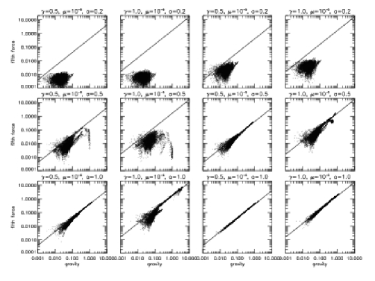
Figure 2: The correlation of the magnitudes of the fifth force and gravity on the CDM particles. The dots denote CDM particles taken from a slice of simulation box with $32.0h^{-1}~{}\mathrm{Mpc}<z<32.1h^{-1}~{}\mathrm{Mpc}$, and the lines are the predicted relation between fifth force and gravity should the former be not suppressed by the chameleon effect. The 4 columns are for the 4 models we consider and the 3 rows are for three output times, respectively $a=0.2,0.5$ and $1$ (corresponding to redshifts 4, 1 and 0) where $a$ is the cosmic scale factor.

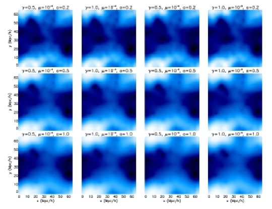
Figure 3: (Colour Online) The gravitational potential on the $z$ plane where $z=32h^{-1}$ Mpc. Dark regions are where the potential is more negative (deeper) while light regions are where it is less negative (shallower). The 4 columns are for the 4 models we consider and the 3 rows are for three output times, respectively $a=0.2,0.5$ and $1$ (corresponding to redshifts 4, 1 and 0) where $a$ is the cosmic scale factor.

Figure 4: (Colour Online) The value of the scalar field $\varphi$ on the $z$ plane where $z=32h^{-1}$ Mpc. Plotted is $\log(\sqrt{\kappa}\varphi)$ for better contrast. Dark regions are where $\varphi$ is closer to 0 while light regions are where it is closer to the background value. The 4 columns are for the 4 models we consider and the 3 rows are for three output times, respectively $a=0.2,0.5$ and $1$ (corresponding to redshifts 4, 1 and 0) where $a$ is the cosmic scale factor.

In Fig. 1 we have shown some snapshots of the distribution of baryonic and CDM particles, to give some idea about the hierachical structure formation and for comparisons with other figures below. It shows clearly how some clustering objects develop, with filaments connecting them together. The baryons roughly follow the clustering of CDM particles, but in some low density regions they become slightly separated.

To understand how the motion of the particles is altered by the coupling to the scalar field, in Fig. 2 we have shown the correlation between the magnitudes of the fifth force and gravity on the CDM particles (remember that baryons do not feel the fifth force). Ref. Li (2009) has made a detailed qualitatively analysis about the general trend of this correction, and here we just give a brief description:

From Eqs. (31, 32) we could see that, when the scalar field potential, i.e., the last term of Eqs. (31, 32) could be neglected, then the scalar field $\varphi$ is simply proportional to the gravitational potential $\Phi$ and as a result Eq. (30) tells us that the strength of the fifth force is just $2\gamma^{2}$ times that of gravity; in other words, the effect of the scalar field is a rescaling of the gravitational constant by $1+2\gamma^{2}$. This is because in this situation, the effective mass of the scalar field, which is given by $m^{2}_{eff}=\partial^{2}V_{eff}/\partial\varphi^{2}$, where

$$V_{eff}(\varphi) = V(\varphi)+C(\varphi)\rho_{\mathrm{CDM}}$$ (38)

is the effective total potential, is light and the fifth force is long-range, like gravity. For comparison, in Fig. 2 we also plot this $2\gamma^{2}$ proportion between the two forces, as a straight line: $\lg(f)=\lg(0.8g)+\lg(2\gamma^{2})$, where $f,g$ denote respectively the magnitudes of the fifth force and gravity, and the factor 0.8 in front of $g$ comes from the fact that only 80% of the particles are CDM (and thus contribute to the fifth force). This scaling relation actually sets an upper limit on how strong the fifth force could be relative to gravity, should it not be suppressed by other effects.

In contrast, when the value of $\varphi$ is small, the last term of Eqs. (31, 32) is not negligible and the scalar field acquires a heavy mass, making it short-ranged. As a result, a particle outside a high density region might not feel the fifth force exerted by particles in that region, even it is quite close to the region. But because it can feel gravity from that region, so the total fifth force on the particle becomes less than the $2\gamma^{2}$ scaling.

In general, the value of $\varphi$ is determined by $\mu,\gamma,\rho_{\mathrm{CDM}}$ as well as its background value $\bar{\varphi}$ (which sets the boundary condition to solve the interior value). At early times $\bar{\varphi}$ is very close to 0 and $\rho_{\mathrm{CDM}}$ is high everywhere, making $\varphi$ small everywhere too, and suppressing the fifth force so that it is significantly below the $2\gamma^{2}$-scaling (first row of Fig. 2). At later times, $\bar{\varphi}$ increases and $\rho_{\mathrm{CDM}}$ decreases, weakening the above effect so that the fifth force becomes ”saturated” (i.e., approaches the $2\gamma^{2}$ prediction) and the points in the figure hit the straight lines (last two rows). Because decreasing $\mu$ and increasing $\gamma$ have the same effects of making $\varphi$ small, in the models with $\mu=10^{-6}$ the fifth force saturates later than in the models with $\mu=10^{-5}$. In addition, because high $\rho_{\mathrm{CDM}}$ tends to decrease $\varphi$ and increase the scalar field mass, so in high density regions (where gravity is stronger) the fifth force also saturates later.

The agreement between the numerical solution of the fifth force and the $2\gamma^{2}$-scaling relation in cases of weak-chameleon effect serves as an independent check of our numerical code.

Fig. 3 plots the spatial configuration for the gravitational potential at the same position and output times as in Fig. 1. As expected, the potential is significantly deeper where there is significant clustering of matter [cf. Fig. 1].

We also show in Fig. 4 the spatial configuration for the scalar field $\varphi$ at the same output position and times. At early times when $\varphi$ is small and the scalar field mass is heavy, the fifth force is so short-ranged that $\varphi$ only depends on the local density. This means that the spatial configuration of $\varphi$ in this situation could well reflect the underlying dark matter distribution, a fact which could be seen clearly in the first row. As time passes by, the mass of the scalar field decreases on average and $\bar{\varphi}$ increases, the value of $\varphi$ at one point is more and more influenced by the matter distribution in neighboring regions, and such an ”averaging” effect weakens the contrast and makes the plots blurring (last two rows). Furthermore, obviously decreasing $\mu$ and increasing $\gamma$ could increase the scalar field’s mass, shorten the range of the fifth force, make $\varphi$ less dependent on its value in neighboring regions, and thus strengthen the contrast in the figures.

III.3 Power Spectrum

To have a more quantitative description about how the matter clustering property is modified with respect to the $\Lambda$CDM model, we consider the matter power spectra $P(k)$ in our simulation boxes.

The nonlinear matter power spectrum in the present work is measured using POWMES Colombi (2009), which is a public available code based on the Taylor expansion of trigonometric functions and yields Fourier modes from a number of fast Fourier transforms controlled by the order of the expansion. We also average the results from the 5 runs for each model and calculate the variance.

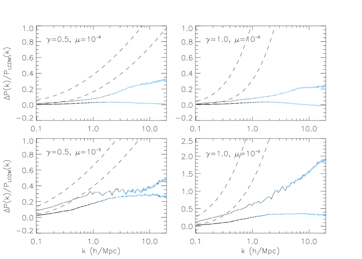
Figure 5: The fractional difference between the nonlinear matter power spectra for the inhomogeneously coupled scalar field model and the $\Lambda$CDM paradigm, where $\Delta P(k)$ is their difference. The range of $k$ is 0.1 to 50 $h$ Mpc^-1. The solid curves are mean and the light-blue error bars the standard deviation calculated from the 5 samples of measurements. Upper solid curves in each panel: the result when $a=1.0$ (redshift 0); Lower solid curves in each panel: the result for $a=0.5$ (redshift 1). The dashed curves are the corresponding results from the linear perturbation theory for comparison.

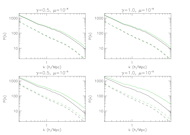
Figure 6: The nonlinear power spectra for CDM and baryonic particles. Shown are the results at two different output times: $a=0.5$ (dashed curves) and $a=1.0$ (solid curves). The upper curves are for CDM particles the lower curves for baryons. Note that we only plot the results in the range $0.1~{}h~{}\mathrm{Mpc}^{-1}\leq k\leq 10~{}h~{}\mathrm{Mpc}^{-1}$ due to the small number of baryonic particles. Note also that all the curves are the mean of 5 relevant runs, but we have not included the standard deviations as in other plots, because they are small and only make the curves unrecognizable.

In Fig. 5 shown are the fractional differences between the $P(k)$ for our 4 models and for $\Lambda$CDM, at two different output times. At early times ($a=0.5$, upper solid curves in each panel), the difference is generally small, but still the 2 models with $\mu=10^{-5}$ show up to $\sim 25\%$ deviation from $\Lambda$CDM prediction. This is because for larger $\mu$ the scalar field is lighter and the fifth force less suppressed, its influence in the structure formation therefore enhanced. Notice that on small scales the deviation from $\Lambda$CDM decreases, which is a desirable property of chameleon models which are designed to suppress the fifth force on small scale high density regions.

The lower solid curves in each panel of Fig. 5 display the same quantities at $a=1.0$ (late times). We can see the trend of increasing deviation from $\Lambda$CDM for all 4 models, because fifth force is essentially unsuppressed at the late epoch [cf. Fig. 2]. For example, the deviation of the model $\gamma=1.0,\mu=10^{-5}$ is significantly larger than that of the model $\gamma=0.5,\mu=10^{-5}$ as naïvely expected, thanks to the lack of suppression of fifth force in both models (the $\gamma=0.5$ model obviously has a smaller saturated fifth force).

For comparison we also plot the $\Delta P/P$ that is predicted by the linear perturbation theory for the 4 models under consideration (the dashed curves). As can be seen there, at large scales (small $k$) where linear perturbation is considered as a good approximation, the linear and nonlinear results agree pretty well (especially for the $a=0.5$ case). The largest scale we can probe is limited by the size of our simulation boxes ($64~{}Mpc/h$) and as a result we cannot make plot beyond the point $k\sim 0.1~{}h/Mpc$, where nonlinearity is expected to first become significant. However, in the case of $a=1.0$, we can see the clear trend of the linear and nonlinear results merging towards $k<0.1~{}h/Mpc$ at vanishing $\Delta P/P$. Similar results can be found in Fig. 2 of Oyaizu (2008) for f(R) gravity.

Because we have two species of matter particles, one uncoupled to the scalar field, we are also interested in their respect power spectrum and the bias between them. These are displayed in Fig. 6. The results could be understood easily: because a CDM particle always feel stronger total force than a baryon at the same position, so the clustering of the former is identically stronger than the latter as well. This could result in a significant bias between these two species at the present time, especially for the models with $\mu=10^{-5}$, where the fifth force is less suppressed.

III.4 Mass Functions

We identify halos in our $N$-body simulations using MHF (MLAPM Halo Finder) Gill (2004), which is the default halo finder for MLAPM. MHF optimally utilizes the refinement structure of the simulation grids to pin down the regions where potential halos reside and organize the refinement hierarchy into a tree structure. Because MLAPM refines grids according to the particle density on them, so the boundaries of the refinements are simply isodensity contours. MHF collect the particles within these isodensity contours (as well as some particles outside). It then performs the following operations: (i) assuming spherical symmetry of the halo, calculate the escape velocity $v_{esc}$ at the position of each particle, (ii) if the velocity of the particle exceeds $v_{esc}$ then it does not belong to the virialized halo and is removed. (i) and (ii) are then iterated until all unbound particles are removed from the halo or the number of particles in the halo falls below a pre-defined threshold, which is 20 in our simulations. Note that the removal of unbound particles is not used in some halo finders using the spherical overdensity (SO) algorithm, which includes the particles in the halo as long as they are within the radius of a virial density contrast. Another advantage of MHF is that it does not require a pre-defined linking length in finding halos, such as the friend-of-friend procedure.

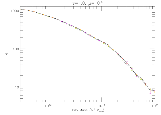
Figure 7: The comparison of three different methods to identify halos from the simulations. The first method (solid curve) uses the approximation Eq. (42) to estimate the escape velocity; the second method (dotted curve) uses the $\Lambda$CDM prediction, which underestimates $v_{esc}$ and causes more particles to be removed; the third method (dashed curve) uses $v_{esc}=\infty$ so that no particles are removed. All curves are for the model $\gamma=1.0,\mu=10^{-5}$, and the curves and error bars denote respectively the mean and standard deviation for 5 sample results.

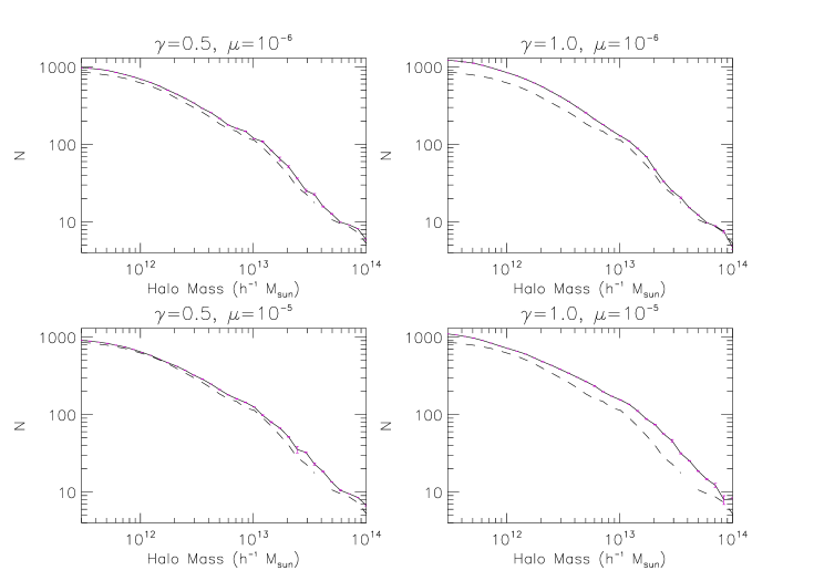
Figure 8: The mass functions for the 4 models under consideration at $a=1.0$ (solid curves). The dashed curve is the mass function for the $\Lambda$CDM simulation. The (solid) curves and error bars denote respectively the mean and standard deviation for 5 sample results.

When it comes to our coupled scalar field model, the MHF algorithm also needs to be modified. The reason is that, as we mentioned above, the scalar field $\varphi$ behaves as an extra ”potential” (which produces the fifth force) and so the CDM particles experience a deeper total ”gravitational” potential than what they do in the $\Lambda$CDM model. Consequently, the escape velocity for CDM particles increases compared with the Newtonian prediction. This is indeed important to bear in mind because, as we have seen in Table 1, the CDM particles are typically much faster than what they are in the $\Lambda$CDM simulation, and so if we underestimate $v_{esc}$ then some particles which should have remained in the halo would be incorrectly removed by MHF. In general, similar things should be taken care of in other theories involving modifications to gravity in the non-relativistic limit, such as MOND and $f(R)$ gravity.

An exact calculation of the escape velocity in the coupled scalar field model is obviously difficult due to the complicated behaviour of the scalar field, and thus here we introduce an approximated algorithm, which is based on the MHF default method Knollmann (2009), to estimate it.

MHF works out $v_{esc}$ using the Newtonian result $v^{2}_{esc}=2|\Phi|$ in which $\Phi$ is the gravitational potential. Under the assumption of spherical symmetry, the Poisson equation $\nabla^{2}\Phi=4\pi G\rho_{m}$ could be integrated once to give

$$\frac{d\Phi}{dr} = \frac{GM(<r)}{r^{2}}$$ (39)

which is just the Newtonian force law. This equation can be integrated once again to obtain

$$\Phi(r) = G\int^{r}_{0}\frac{M(<r^{\prime})}{r^{\prime 2}}dr^{\prime}+\Phi_{0}$$ (40)

where $\Phi_{0}$ is an integration constant and can be fixed Knollmann (2009) by requiring that $\Phi(r=\infty)=0$ as

$$\Phi_{0} = \frac{GM_{vir}}{R_{vir}}+G\int^{R_{vir}}_{0}\frac{M(<r^{\prime})}{r^{\prime 2}}dr^{\prime},$$ (41)

in which $R_{vir}$ is the virial radius of the halo and $M_{vir}$ is the mass enclosed in $R_{vir}$.

When the fifth force acts on CDM particles, the force law Eq. (39) is modified and these particles feel a larger total ”gravitational” potential. To take this into account, we need to have the knowledge about how the force law is modified and a simple rescaling of gravitational constant $G$ has been shown to be not physical in certain regimes.

To solve the problem, we notice that in the MHF code Eq. (39) is used in the numerical integrations to obtain both $\Phi(r)$ and $\Phi_{0}$ [cf. Eqs.(40, 41)]. More explicitly, the code loops over all particles in the halo in ascending order of the distance from the halo centre, and when a particle is encountered its mass is uniformly distributed into the spherical shell between the particle and its previous particle (the thickness of the shell is then the $dr$ of the integration). Obviously when the fifth force is added into Eq. (39) we could use the same method to compute the total ”gravitational” potential which includes the contribution from $\varphi$ (call this contribution $\Phi_{\varphi}$; because $d\Phi_{\varphi}/dr=\mathrm{fifth~{}force}$, so from Eq. (26) we can easily see $\Phi_{\varphi}=\frac{C_{,\varphi}}{C}a\varphi$). But now there is a subtlety here: not all particles are CDM while only CDM particles contribute to $\Phi_{\varphi}$. So in the modified MHF code we calculate $\Phi,\Phi_{0}$ and $\Phi_{\varphi},\Phi_{\varphi 0}$ separately, using all particles for the former and only CDM for the latter. Finally

$$v_{esc}^{2} = 2|\Phi+\Phi_{\varphi}-\Phi_{0}-\Phi_{\varphi 0}|$$ (42)

is our estimate of the escape velocity. Because we have recorded the components of gravity and the fifth force for each particle in the simulation, so the fifth-force-to-gravity ratio can be computed at the position of each particle, which is approximated to be $\left(\Phi_{\varphi}-\Phi_{\varphi 0}\right)/\left(\Phi-\Phi_{0}\right)$ at that position. In this way we have, at least approximately, taken into account the environment dependence of the fifth force and thus of $\Phi_{\varphi}$.

To see how our modification of the MHF code affects the final result on the mass function, in Fig. 7 we compare the mass functions for the model $\gamma=1.0,\mu=10^{-5}$ calculated using three methods: the modified MHF, the original MHF (by default for $\Lambda$CDM simulations) and another modified MHF in which we set $v_{esc}$ to be very large so that no particles will ever escape from any halo (this is similar to the spherical overdensity algorithm mentioned above). It could be seen that the difference between these methods can be up to a few percent for small halos where the potential is shallow, particle number is small and the result is sensitive to whether more particles are removed. As expected, the second method gives least halos because there $v_{esc}$ is smallest and many particles are removed, while the third method gives most halos because no particles are removed at all.

Fig. 8 displays the mass functions for the 4 models as compared to the $\Lambda$CDM result. As expected, the fifth force enhances the structure formation and thus produces more halos in the simulation box.

III.5 Halo Profiles

As our simulations have reached a force resolution of $\sim 12h^{-1}$ kpc, while the typical size of the large halos in the simulations is of order Mpc, we could ask what the internal profiles of the halos look like and how they have been modified by the coupling between CDM particles and the scalar field.

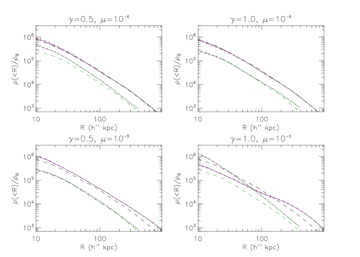
Figure 9: The overdensity inside two typical halos selected from the simulations for each model (see text for a more detailed description), as a function of the halo radius $R$. The solid curves and error bars denote respectively the mean and standard deviation for the results from our 5 sample runs, while the dashed curve is the $\Lambda$CDM prediction. In each panel the upper two curves (black) at large radii are for halo I and the lower two curves (green) at large radii are for halo II. $\rho_{\mathrm{B}}$ is the background matter (baryons and CDM) density. We skipped the result for $R<10h^{-1}$ kpc, which is not reliable due to the limit from resolution.

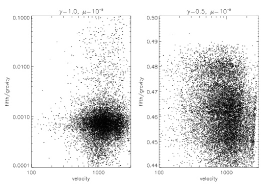
Figure 10: Distribution of the velocities of the particles in halo I and the fifth-force-to-gravity ratio at the positions of these particles, for the two models $\gamma=0.5,\mu=10^{-5}$ and $\gamma=1.0,\mu=10^{-5}$. Each dots represent a particle.

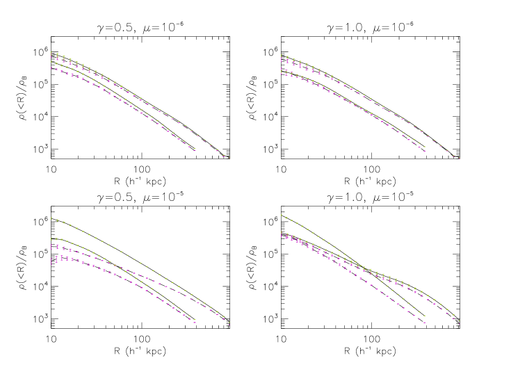
Figure 11: The CDM and baryonic overdensities inside the two halos selected above, as a function of the halo radius $R$. The solid curves and error bars denote respectively the mean and standard deviation for the CDM results from our 5 sample runs, while the dashed curve and error bars are for baryons. In each panel the upper two curves are for halo I and the lower two curves are for halo II. $\rho_{\mathrm{B}}$ is the background matter (baryons and CDM) density. We skipped the result for $R<10h^{-1}$ kpc, which is not reliable due to the limit from resolution.

We have selected 2 typical halos from each simulation. Halo I is centred on $(x,y,z)\sim(27.0,32.2,17.8)h^{-1}$ Mpc, which is slightly different for different simulations, and has a virial mass $M_{vir}\sim 1.16\times 10^{14}h^{-1}~{}M_{\bigodot}$; halo II is centred on $(x,y,z)\sim(52.5,62.9,38.3)h^{-1}$ Mpc, which is also slightly different for different simulations, and has a virial mass $M_{vir}\sim 1.70\times 10^{13}h^{-1}~{}M_{\bigodot}$ (note here that the virial masses are for the $\Lambda$CDM simulations, and for scalar field simulations they can be, and generally are, slightly different).

The largest halos, such as halo I, generally reside in the higher density regions where the scalar field has a heavier mass and shows stronger chameleon effect. Consequently the fifth force inside them is severely suppressed so that we can expect small deviation from the $\Lambda$CDM halo profile. On the other hand, the intermediate and small halos (such as halo II) are mostly in relatively low density regions in which scalar field has a light mass and the fifth force tends to saturate; this means that they should generally have a higher internal density than the same halos in the $\Lambda$CDM simulation due to the enhanced growth by the fifth force.

This above analysis is qualitatively confirmed by Fig. 9, where we can see that for the cases of $\mu=10^{-6}$ (stronger chameleon) the difference between the predictions of the coupled scalar field models and the $\Lambda$CDM paradigm is really small for halo I. Furthermore, this figure also shows some new and more interesting features for the cases of $\mu=10^{-5}$. Considering halo I in the models $\gamma=0.5,\mu=10^{-5}$ and $\gamma=1.0,\mu=10^{-5}$ for example: in the former case, the coupled scalar field model produces an obviously consistent higher internal density profile than $\Lambda$CDM, from the inner to the outer regions of the halo; while for the latter case, the density profile of the coupled scalar field model is lower in the inner region but higher in the outer region!

We plan to make a detailed analysis of the complexities arising here regarding the effects of a coupled scalar field on the internal density profiles for halos in a future work, and in this work we will only give a brief explanation for the new feature observed above: Fig. 10 shows the distributions of particle velocities and fifth-force-to-gravity ratio at the positions of the particles in halo I for the two models $\gamma=0.5,\mu=10^{-5}$ and $\gamma=1.0,\mu=10^{-5}$. As we can see there, for the model $\gamma=1.0,\mu=10^{-5}$ the large value of $\gamma$ makes the chameleon effect strong so that the fifth force is generally much smaller than gravity in magnitude, while at the same time the velocities of particles are more concentrated towards the high end, implying a significantly higher mean speed than $\Lambda$CDM (as we have checked numerically); as a result in the central region of the halo the particles have higher kinetic energy than in $\Lambda$CDM but the potential is not significantly deeper, so that particles tend to get far away from the centre of the halo, producing a lower inner density profile. As for the model with $\gamma=0.5,\mu=10^{-5}$, the situation is just the opposite: the fifth force is saturated and of the same order as gravity due to the weak chameleon effect, so that the total potential is greatly deeper than its $\Lambda$CDM counterpart, while at the same time the particles are not as fast as those in $\gamma=1.0,\mu=10^{-5}$: the consequence is that the halo accretes more particles towards its centre.

One might also have interests in how the CDM part and the baryonic part of the halo profile differ from each other, and this is given in Fig. 11, in which we compare the CDM and baryon density profiles of halos I and II. Obviously the CDM density is higher than baryons everywhere, again thanks to the boost from the fifth force. For smaller $\mu$ and larger $\gamma$ (which help strengthen the chameleon effect and suppress the fifth force), the difference between the two is smaller (compare the halo I in the models $\gamma=0.5,\mu=10^{-5}$ and $\gamma=1.0,\mu=10^{-5}$). However, in the situations where the fifth force is already saturated or unsuppressed (such as in halo II), increasing $\gamma$ increases the saturated value of the fifth force, and thus can instead magnify the difference (compare the halo II in the models $\gamma=0.5,\mu=10^{-5}$ and $\gamma=1.0,\mu=10^{-5}$).

The above results again show the complexity of the chameleon scalar field model as compared to other coupled scalar field models. We will study the environment and epoch dependence of the halo density profiles in a upcoming work.

IV Discussion and Conclusion

To summarize, in this paper we have investigated into a model where CDM and baryons couple differently to a chameleon-like scalar field, and performed full $N$-body simulations, by directly solving the spatial distribution of the scalar field, to study the nonlinear structure formation under this setup. The new complexity introduced here compared to Li (2009) is that we must distinguish between baryons and CDM so that we know how to calculate the force upon each particle. We do this by tagging the initial almost homogeneously distributed particle randomly so that 80% of all particles are tagged as CDM. We then only use CDM particles to calculate the scalar field and only applies the fifth scalar force on CDM particles.

The coupling function (characterized by the coupling strength $\gamma$) and bare potential (characterized by the parameter $\mu$ which controls its steepness) of the scalar field are chosen to be the same as in Li (2009). As discussed there, the coupling of the scalar field to CDM particles acts on the latter a fifth force. When $\mu$ is small and $\gamma$ is large, the chameleon effect becomes stronger, which gives the scalar field a heavy mass, making the fifth force short-ranged and the scalar field dependent only on the local matter density. Other ways to strengthen the chameleon effect includes increasing the density and decreasing the background value of the scalar field, which itself is equivalent to increasing the background CDM energy density. We have displayed in Figs. 2, 4 how changing the determining factors change the scalar field configuration and the strength of the fifth force.

We have also measured the nonlinear matter power spectrum from the simulation results and compared them with the $\Lambda$CDM prediction. Depending on the values of $\gamma,\mu$ as well as the background CDM density, the former can be up to $\sim 80\%$ larger than the latter. Nonetheless, when the chameleon effect is set to be strong, the deviation gets suppressed and in particular decreases towards small scales, showing the desirable property of chameleon models that they evade constraints on small scales. The bias between CDM and baryons power spectra follows the same trend.

To identify virialized halos from the simulations, we have modified MHF, MLAPM’s default halo finder, so that the calculation of the escape velocity includes the effect of the scalar field. We find that such a modification leads to up to a-few-percent enhancement on the mass function compared with what is obtained using the default MHF code, because in the latter case the escape velocity is underestimated and some particles are incorrectly removed from the virialized halos. We find that the mass function in the coupled scalar field models is significantly larger than the $\Lambda$CDM result, because of the enhanced structure growth induced by the fifth force.

Finally, we have analyzed the internal profiles of (the same) two halos selected from each simulation. We find that when chameleon effect is strong and fifth force is suppressed, our result is very close to the $\Lambda$CDM prediction; this is the case for very large halos (which generally reside in higher density regions) and $\mu=10^{-6}$. For large halos and $\mu=10^{-5}$, the situation is more complicated because the competition between two effects of the coupled scalar field, namely the speedup of the particles and the deepening of the total attractive potential, has arrived a critical point: if the former wins, such as in the model $\gamma=1.0,\mu=10^{-5}$, then the inner density profile can be lower than that in $\Lambda$CDM; if the latter wins, such as in the model $\gamma=1.0,\mu=10^{-5}$, then we expect the opposite. For smaller halos which locate in lower density regions, the fifth force is not suppressed that much and causes faster growth of the structure, so the halo is more concentrated and has a higher internal density. Meanwhile, the bias between baryons and CDM density profiles also increase as the fifth force becomes less suppressed, which is as expected.

Our results already show that new features can be quantitatively studied with the $N$-body method and the improving supercomputing techniques, and that the chameleon model has rather different consequences from other coupled scalar field models. The enhancement in the structure formation due to the fifth force is significant for some of our parameter space, which means other observables, such as weak lensing, could place new constraints on the model. Also one might be interested in how the halo profiles would be like at different epoch of the cosmological evolution and in different environments. These will be left as future work.

Appendix A Discretized Equations for Our $N$-body Simulations

In the MLAPM code the partial differential equation Eq. (31) is (and in our modified code Eq. (32) will also be) solved on discretized grid points, and as such we must develop the discretized versions of Eqs. (29 - 32) to be implemented into the code.

But before going on to the discretization, we need to address a technical issue. As the potential is highly nonlinear, in the high density regime the value of the scalar field $\sqrt{\kappa}\varphi$ will be very close to 0, and this is potentially a disaster as during the numerical solution process the value of $\sqrt{\kappa}\varphi$ might easily go into the forbidden region $\varphi<0$ Oyaizu (2008). One way of solving this problem is to define $\chi=\bar{\chi}e^{u}$ in which $\bar{\chi}$ is the background value of $\chi$, as in Oyaizu (2008). Then the new variable $u$ takes value in $(-\infty,\infty)$ so that $e^{u}$ is positive definite which ensures that $\chi>0$. However, since there are already exponentials of $\chi$ in the potential, this substitution will result terms involving $\exp\left[\exp(u)\right]$, which could potentially magnify any numerical error in $u$.

Instead, we can define a new variable $u$ according to

$$e^{u}+1 = e^{\chi}.$$ (43)

By this, $u$ still takes value in $(-\infty,\infty)$, $e^{u}\in(0,\infty)$ and thus $e^{\chi}\in(1,\infty)$ which ensures that $\chi$ is positive definite in numerical solutions. Besides, $e^{\beta\chi}=\left[1+e^{u}\right]^{\beta}$ so that there will be no exponential-of-exponential terms, and the only exponential is what we have for the potential itself. $\beta=-1$ above.

Then the Poisson equation becomes

$$\nabla^{2}\Phi_{c}$$ (44)

$$= \frac{3}{2}\Omega_{\mathrm{CDM}}\left[\rho_{c,\mathrm{CDM}}\left(1+e^{u}\right)^{\gamma}-e^{\gamma\sqrt{\kappa}\bar{\varphi}}\right]$$

$$+\frac{3}{2}\Omega_{\mathrm{B}}\left(\rho_{c,\mathrm{B}}-1\right)-\frac{3\Omega_{V_{0}}a^{3}}{\left[1-\left(1+e^{u}\right)^{\beta}\right]^{\mu}}+3\bar{\Omega}_{V}a^{3},\ \ \ \ \$$

where we have defined $\bar{\Omega}_{V}=\kappa V(\bar{\varphi})/3H_{0}^{2}$ which is determined by background cosmology, the quantity $e^{\gamma\sqrt{\kappa}\bar{\varphi}}$ is also determined solely by background cosmology. These background quantities should not bother us here.

The scalar field EOM becomes

$$\frac{ac^{2}}{\left(H_{0}B\right)^{2}}\nabla\cdot\left(\frac{e^{u}}{1+e^{u}}\nabla u\right)$$ (45)

$$= 3\gamma\Omega_{\mathrm{CDM}}\rho_{c,\mathrm{CDM}}\left(1+e^{u}\right)^{\gamma}+\frac{3\mu\beta\Omega_{V_{0}}a^{3}\left(1+e^{u}\right)^{\beta}}{\left[1-\left(1+e^{u}\right)^{\beta}\right]^{\mu+1}}$$

$$-3\gamma\Omega_{\mathrm{CDM}}e^{\gamma\sqrt{\kappa}\bar{\varphi}}-\frac{3\mu\beta\Omega_{V_{0}}a^{3}e^{\beta\sqrt{\kappa}\bar{\varphi}}}{\left[1-e^{\beta\sqrt{\kappa}\bar{\varphi}}\right]^{m+1}}$$

in which we have used the fact that $\chi=\log(1+e^{u})\Rightarrow\nabla\chi=\frac{e^{u}}{1+e^{u}}\nabla u$, and moved all terms depending only on background cosmology (the source terms) to the right hand side.

So, in terms of the new variable $u$, the set of equations used in the $N$-body code should be

$$\frac{d\mathbf{x}_{c}}{dt_{c}} = \frac{\mathbf{p}_{c}}{a^{2}},$$ (46)

$$\frac{d\mathbf{p}_{c}}{dt_{c}} = -\frac{1}{a}\nabla\Phi_{c}\left[-\frac{c^{2}\gamma}{\left(H_{0}B\right)^{2}}\frac{e^{u}}{1+e^{u}}\nabla u\right]$$ (47)

plus Eqs. (44, 45). These equations will ultimately be used in the code. Among them, Eqs. (44, 47) will use the value of $u$ while Eq. (45) solves for $u$. In order that these equations can be integrated into MLAPM, we need to discretize Eq. (45) for the application of Newton-Gauss-Seidel iterations.

To discretize Eq. (45), let us define $b\equiv\frac{e^{u}}{1+e^{u}}$. The discretization involves writing down a discretion version of this equation on a uniform grid with grid spacing $h$. Suppose we require second order precision as is in the standard Poisson solver of MLAPM, then $\nabla u$ in one dimension can be written as

$$\nabla u \rightarrow \nabla^{h}u_{j}\ =\ \frac{u_{j+1}-u_{j-1}}{2h}$$ (48)

where a subscript _j means that the quantity is evaluated on the $j$-th point. Of course the generalization to three dimensions is straightforward.

The factor $b$ in $\nabla\cdot\left(b\nabla u\right)$ makes this a standard variable coefficient problem. We need also discretize $b$, and do it in this way (again for one dimension):

$$\nabla\cdot\left(b\nabla u\right) \rightarrow \left(\nabla^{h}b_{j}\right)\cdot\left(\nabla^{h}u_{j}\right)+b_{j}\nabla^{h2}u_{j}$$ (49)

$$= \frac{b_{j+1/2}-b_{j-1/2}}{h}\frac{u_{j+1}-u_{j-1}}{2h}+\frac{b_{j+1/2}+b_{j-1/2}}{2}\frac{u_{j+1}-2u_{j}+u_{j-1}}{h^{2}}$$

$$= \frac{1}{h^{2}}\left[b_{j+\frac{1}{2}}u_{j+1}-u_{j}\left(b_{j+\frac{1}{2}}+b_{j-\frac{1}{2}}\right)+b_{j-\frac{1}{2}}u_{j-1}\right]$$

where we have defined $b_{j+\frac{1}{2}}=\left(b_{j}+b_{j+1}\right)/2$ and $b_{j-\frac{1}{2}}=\left(b_{j-1}+b_{j}\right)/2$. This can be easily generalize to three dimensions as

$$\nabla\cdot\left(b\nabla u\right) \rightarrow \frac{1}{h^{2}}\left[b_{i+\frac{1}{2},j,k}u_{i+1,j,k}-u_{i,j,k}\left(b_{i+\frac{1}{2},j,k}+b_{i-\frac{1}{2},j,k}\right)+b_{i-\frac{1}{2},j,k}u_{i-1,j,k}\right]$$ (50)

$$+\frac{1}{h^{2}}\left[b_{i,j+\frac{1}{2},k}u_{i,j+1,k}-u_{i,j,k}\left(b_{i,j+\frac{1}{2},k}+b_{i,j-\frac{1}{2},k}\right)+b_{i,j-\frac{1}{2},k}u_{i,j-1,k}\right]$$

$$+\frac{1}{h^{2}}\left[b_{i,j,k+\frac{1}{2}}u_{i,j,k+1}-u_{i,j,k}\left(b_{i,j,k+\frac{1}{2}}+b_{i,j,k-\frac{1}{2}}\right)+b_{i,j,k-\frac{1}{2}}u_{i,j,k-1}\right].$$

Then the discrete version of Eq. (45) is

$$L^{h}\left(u_{i,j,k}\right) = 0,$$ (51)

in which

$$L^{h}\left(u_{i,j,k}\right) = \frac{1}{h^{2}}\left[b_{i+\frac{1}{2},j,k}u_{i+1,j,k}-u_{i,j,k}\left(b_{i+\frac{1}{2},j,k}+b_{i-\frac{1}{2},j,k}\right)+b_{i-\frac{1}{2},j,k}u_{i-1,j,k}\right]$$ (52)

$$+\frac{1}{h^{2}}\left[b_{i,j+\frac{1}{2},k}u_{i,j+1,k}-u_{i,j,k}\left(b_{i,j+\frac{1}{2},k}+b_{i,j-\frac{1}{2},k}\right)+b_{i,j-\frac{1}{2},k}u_{i,j-1,k}\right]$$

$$+\frac{1}{h^{2}}\left[b_{i,j,k+\frac{1}{2}}u_{i,j,k+1}-u_{i,j,k}\left(b_{i,j,k+\frac{1}{2}}+b_{i,j,k-\frac{1}{2}}\right)+b_{i,j,k-\frac{1}{2}}u_{i,j,k-1}\right]$$

$$-\frac{\left(H_{0}B\right)^{2}}{ac^{2}}\left[3\gamma\Omega_{\mathrm{CDM}}\rho^{\mathrm{CDM}}_{c,i,j,k}\left(1+e^{u_{i,j,k}}\right)^{\gamma}+\frac{3\mu\beta\Omega_{V_{0}}a^{3}\left(1+e^{u_{i,j,k}}\right)^{\beta}}{\left[1-\left(1+e^{u_{i,j,k}}\right)^{\beta}\right]^{\mu+1}}\right]$$

$$+\frac{\left(H_{0}B\right)^{2}}{ac^{2}}\left[3\gamma\Omega_{\mathrm{CDM}}e^{\gamma\sqrt{\kappa}\bar{\varphi}}+\frac{3\mu\beta\Omega_{V_{0}}a^{3}e^{\beta\sqrt{\kappa}\bar{\varphi}}}{\left[1-e^{\beta\sqrt{\kappa}\bar{\varphi}}\right]^{\mu+1}}\right].$$

Then the Newton-Gauss-Seidel iteration says that we can obtain a new (and often more accurate) solution of $u$, $u^{\mathrm{new}}_{i,j,k}$, using our knowledge about the old (and less accurate) solution $u^{\mathrm{old}}_{i,j,k}$ as

$$u^{\mathrm{new}}_{i,j,k} = u^{\mathrm{old}}_{i,j,k}-\frac{L^{h}\left(u^{\mathrm{old}}_{i,j,k}\right)}{\partial L^{h}\left(u^{\mathrm{old}}_{i,j,k}\right)/\partial u_{i,j,k}}.$$ (53)

The old solution will be replaced by the new solution to $u_{i,j,k}$ once the new solution is ready, using the red-black Gauss-Seidel sweeping scheme. Note that

$$\frac{\partial L^{h}(u_{i,j,k})}{\partial u_{i,j,k}} = \frac{1}{2h^{2}}\frac{e^{u_{i,j,k}}}{\left(1+e^{u_{i,j,k}}\right)^{2}}\left[u_{i+1,j,k}+u_{i-1,j,k}+u_{i,j+1,k}+u_{i,j-1,k}+u_{i,j,k+1}+u_{i,j,k-1}-6u_{i,j,k}\right]$$ (54)

$$-\frac{1}{2h^{2}}\left[b_{i+1,j,k}+b_{i-1,j,k}+b_{i,j+1,k}+b_{i,j-1,k}+b_{i,j,k+1}+b_{i,j,k-1}+6b_{i,j,k}\right]$$

$$-\frac{\left(H_{0}B\right)^{2}}{ac^{2}}3\gamma^{2}\Omega_{\mathrm{CDM}}\rho^{\mathrm{CDM}}_{c,i,j,k}\left(1+e^{u_{i,j,k}}\right)^{\gamma}b_{i,j,k}$$

$$-\frac{\left(H_{0}B\right)^{2}}{ac^{2}}\frac{3\mu\beta^{2}\Omega_{V_{0}}a^{3}\left(1+e^{u_{i,j,k}}\right)^{\beta}}{\left[1-\left(1+e^{u_{i,j,k}}\right)^{\beta}\right]^{\mu+1}}b_{i,j,k}\left[1+(\mu+1)\frac{\left(1+e^{u_{i,j,k}}\right)^{\beta}}{1-\left(1+e^{u_{i,j,k}}\right)^{\beta}}\right].$$

In principle, if we start from a high redshift, then the initial guess of $u_{i,j,k}$ could be such that the initial value of $\chi$ in all the space is equal to the background value $\bar{\chi}$, because anyway at this time we expect this to be approximately true. For subsequent time steps we could use the solution for $u_{i,j,k}$ at the previous time step as our initial guess; if the time step is small enough then we do not expect $u$ to change significantly between consecutive times so that such a guess will be good enough for the iteration to converge fast.

In practice, however, due to specific features and algorithm of the MLAPM code Knebe (2001), the above procedure may be slightly different in details.