Abstract

It has recently been shown that by measuring the transverse polarizations of the final particles in $\mu^{+}\to e^{+}e^{-}e^{+}$, it is possible to extract information on the phases of the effective couplings leading to this decay. We examine this possibility within the context of $R$-parity violating Minimal Supersymmetric Standard Model (MSSM) in which the $\mu^{+}\to e^{+}e^{-}e^{+}$ process can take place at a tree level. We demonstrate how a combined analysis of the angular distribution of the emitted electrons and their transverse polarization can determine the CP-violating phases of the trilinear R-parity violating Yukawa couplings.

1 Introduction

If the neutrino masses are the only sources of Lepton Flavor Violation (LFV), the rates of the Lepton Flavor Violating processes such as $\mu\to e\gamma$, $\mu N\to eN$ and $\mu\to eee$ will be too small to be detectable in the foreseeable future. Any positive signal for such LFV processes will be an indication for new physics beyond the Standard Model (SM). Strong experimental bounds exist on the rate of these processes [1] and rich literature has been developed on the constraints on new physics from these bounds. Currently, the MEG experiment at PSI is searching for $\mu\to e\gamma$ and will be able to detect a signal even if Br$(\mu\to e\gamma)$ is as small as $O(10^{-13})$.

We can divide the beyond SM scenarios into two classes: (1) Models, such as R-parity conserving Minimal Supersymmetric Standard Model (MSSM), within which only even numbers of new particles can appear in each vertex; (2) Models, such as R-parity violating MSSM, within which the number of new particles in each vertex can be both even or odd. In case of the first class of models, both $\mu\to e\gamma$ and $\mu\to eee$ can take place only at the loop level. Within these models Br($\mu\to eee$), being a three body decay, is typically smaller than Br($\mu\to e\gamma$) so the latter gives stronger bounds on the LFV parameters (see, however [2]). However, within the second class of the models, $\mu\to eee$ can take place at tree level and its rate can therefore exceed that of $\mu\to e\gamma$ which is possible only at a loop level. Within the R-parity violating MSSM, it is possible that while Br($\mu\to e\gamma$) is too small to be probed even by MEG, Br($\mu\to eee$) is relatively large and close to its present bound [2]. A mild improvement on $\mu\to eee$ can probe R-parity violating MSSM with mass scale well above 10 TeV which is beyond the reach of the LHC.

Recently it has been shown that by measuring the transverse polarizations of the final particles in $\mu\to e\gamma$, $\mu-e$ conversion on nuclei and $\mu\to eee$, one can measure the CP-violating phases of the general effective Lagrangian leading to these processes [3, 4, 5]. The possibility of deriving information on the CP-violating phases of the R-parity conserving MSSM from $\mu\to e\gamma$ and the $\mu-e$ conversion has been explored in [4]. In the present letter, we are going to examine the possibility of deriving the CP-violating phases of the trilinear R-parity violating couplings from $\mu\to eee$. These CP-violating phases are important as they can be responsible for the creation of the baryon asymmetry in the universe [6].

The paper is organized as follows. In section 2, we review the general effective Lagrangian that can lead to $\mu\to eee$ and $\mu\to e\gamma$. We outline the information that can be derived on the effective couplings without the measurement of the spin of the final particles. In section 3, we review the contributions that the effective couplings receive from the $R$-parity and lepton flavor violating trilinear Yukawa couplings. We then briefly review bounds on these couplings. In section 4, we introduce the P-odd asymmetry, $\mathcal{A}$, and the transverse polarization. In section 5, we briefly discuss the feasibility of measuring the transverse polarization of the final particles. In section 6, we discuss the results that can be derived by combined analysis of $\mathcal{A}$ and the transverse polarization. Results are summarized in section 7.

2 Effective Lagrangian in a general framework

The effective Lagrangian leading to $\mu\to eee$ can in general be written as [7]

$${\cal L}_{\rm eff} = B_{1}(\bar{\mu}_{L}e_{R})(\bar{e}_{R}e_{L})+B_{2}(\bar{\mu}_{R}e_{L})(\bar{e}_{L}e_{R})+\ \ \$$ (1)

$$C_{1}(\bar{\mu}_{L}e_{R})(\bar{e}_{L}e_{R})+C_{2}(\bar{\mu}_{R}e_{L})(\bar{e}_{R}e_{L})+$$ (2)

$$G_{1}(\bar{\mu}_{R}\gamma^{\nu}e_{R})(\bar{e}_{R}\gamma_{\nu}e_{R})+G_{2}(\bar{\mu}_{L}\gamma^{\nu}e_{L})(\bar{e}_{L}\gamma_{\nu}e_{L})$$ (3)

$$-A_{R}\leavevmode\nobreak\ (\bar{\mu}_{L}[\gamma_{\mu},\gamma_{\nu}]\leavevmode\nobreak\ \frac{q^{\nu}}{q^{2}}e_{R})\leavevmode\nobreak\ (\bar{e}\gamma^{\mu}e)-A_{L}\leavevmode\nobreak\ (\bar{\mu}_{R}[\gamma_{\mu},\gamma_{\nu}]\leavevmode\nobreak\ \frac{q^{\nu}}{q^{2}}e_{L})\leavevmode\nobreak\ (\bar{e}\gamma^{\mu}e)+{\rm H.c.}$$ (4)

Notice that by using the identities $(\sigma^{\mu})_{\alpha\beta}(\sigma_{\mu})_{\gamma\delta}\equiv 2\epsilon_{\alpha\gamma}\epsilon_{\beta\delta}$ and $(\bar{\sigma}^{\mu})_{\alpha\beta}=\epsilon_{\beta\delta}(\sigma^{\mu})_{\delta\gamma}\epsilon_{\gamma\alpha}$ (where $\epsilon_{11}=\epsilon_{00}=0$ and $\epsilon_{10}=-\epsilon_{01}=1$) and employing the fact that the fermions anti-commute, we can rewrite the terms on the first line of Eq. (1) as

$$-{B_{1}\over 2}(\bar{\mu}_{L}\gamma^{\nu}e_{L})(\bar{e}_{R}\gamma_{\nu}e_{R})-{B_{2}\over 2}(\bar{\mu}_{R}\gamma^{\nu}e_{R})(\bar{e}_{L}\gamma_{\nu}e_{L})\ .$$

This effective Lagrangian leads to [7]

$$Br(\mu\to eee) = {1\over 32G_{F}^{2}}\left[|B_{1}|^{2}+|B_{2}|^{2}+8(|G_{1}|^{2}+|G_{2}|^{2})\right.$$ (5)

$$+ {|C_{1}|^{2}+|C_{2}|^{2}\over 2}+32(4\log{m_{\mu}^{2}\over m_{e}^{2}}-{11}){|A_{R}|^{2}+|A_{L}|^{2}\over m_{\mu}^{2}}$$ (6)

$$- \left.64{\Re[A_{L}G_{2}^{*}+A_{R}G_{1}^{*}]\over m_{\mu}}+32{\Re[A_{L}B_{1}^{*}+A_{R}B_{2}^{*}]\over m_{\mu}}\right]\ .$$ (7)

By studying the energy distribution of the final particles, more information can be derived on the effective couplings. For example, let us consider the contributions from $A_{L}$ and $A_{R}$ which come from a virtual photon exchange. When the invariant mass of an electron positron pair goes to zero, the virtual exchanged photon goes on shell. As a result, the corresponding Dalitz plot should have a peak at $(P_{e^{-}}+P_{e^{+}})^{2}=0$ whose height is given by $|A_{L}|^{2}+|A_{R}|^{2}$. The combinations that can be derived by studying the energy distributions of the final particles are $|G_{1}|^{2}+|G_{2}|^{2}+(|C_{1}|^{2}+|C_{2}|^{2})/16$, $|B_{1}|^{2}+|B_{2}|^{2}$, $|A_{L}|^{2}+|A_{R}|^{2}$, ${\rm Re}[A_{L}G_{2}^{*}+A_{R}G_{1}^{*}]$ and ${\rm Re}[A_{L}B_{1}^{*}+A_{R}B_{2}^{*}]$ (see for example [7] and references therein). By studying the angular distributions of the final particles relative to the polarization of the initial muon, one can further derive $|G_{1}|^{2}-|G_{2}|^{2}+(-|C_{1}|^{2}+|C_{2}|^{2})/16$, $|B_{1}|^{2}-|B_{2}|^{2}$, $|A_{L}|^{2}-|A_{R}|^{2}$, ${\rm Re}[A_{L}G_{2}^{*}-A_{R}G_{1}^{*}]$ and ${\rm Re}[A_{L}B_{1}^{*}-A_{R}B_{2}^{*}]$ as well as the CP-odd quantities ${\rm Im}[A_{L}G_{2}^{*}+A_{R}G_{1}^{*}]$ and ${\rm Im}[A_{L}B_{1}^{*}+A_{R}B_{2}^{*}]$. A combined analysis of angular and energy distribution therefore yields the absolute values of all the effective couplings, $B_{1}$, $B_{2}$, $A_{L}$ and $A_{R}$ as well as the CP-violating phases $\arg[A_{L}A_{R}^{*}G_{2}^{*}G_{1}]$, $\arg[A_{L}G_{2}^{*}]$, $\arg[A_{L}A_{R}^{*}B_{1}^{*}B_{2}]$ and $\arg[A_{L}B_{1}^{*}]$. Notice however that there is still some information in Eq. (1) that cannot be derived by the methods described above. In particular, the CP-violating phase arg$[B_{1}B_{2}^{*}]$ cannot be derived by these methods. Further information can be obtained by studying the transverse polarization of $e^{-}$ in $\mu^{+}\to e^{+}e^{-}e^{+}$ [3].

Notice that the terms on the last line of Eq. (1) come from the effective coupling of the photon which gives rise to

$${\rm Br}(\mu\to e\gamma)=\frac{12\pi}{G_{F}^{2}m_{\mu}^{2}\alpha}\left(|A_{L}|^{2}+|A_{R}|^{2}\right)\ .$$ (8)

The present bound on this LFV rare decay is very strong ${\rm Br}(\mu\to e\gamma)<1.2\times 10^{-11}$ [1] which implies $|A_{L}|^{2}+|A_{R}|^{2}<3.3\times{10^{-27}}\leavevmode\nobreak\ {\rm GeV}^{-2}$. Thus, from Eq. (3), we observe that the contribution from $A_{L}$ and $A_{R}$ to $\mu\to eee$ cannot be larger than $7\times 10^{-14}$ so if Br($\mu\to eee$) turns out to be close to its present bound, we can safely neglect the contributions from $A_{L}$ and $A_{R}$.

3 Effects of trilinear R-parity violating couplings

Within the R-parity conserving MSSM, the slepton mass matrix as well as the trilinear $A$-term involving the sleptons include LFV sources which can induce the effective Lagrangian in Eq. (1). By relaxing the R-parity conservation, new sources of LFV emerge. In particular, the R-parity violating Yukawa couplings in the superpotential

$$W={\lambda_{ijk}\over 2}\hat{L}_{i}\hat{L}_{j}\hat{E}_{k}\leavevmode\nobreak\ \leavevmode\nobreak\ \leavevmode\nobreak\ \leavevmode\nobreak\ \leavevmode\nobreak\ {\rm with}\leavevmode\nobreak\ \leavevmode\nobreak\ \leavevmode\nobreak\ \leavevmode\nobreak\ \leavevmode\nobreak\ \lambda_{ijk}=-\lambda_{jik}\$$ (9)

add nine new sources of LFV. That is each nonzero element of $\lambda_{ijk}$ is a source of LFV. Some of these couplings can contribute to $\mu\to eee$ at tree level. Throughout this letter, we will focus on the effects of $\lambda$ and set other LFV sources equal to zero for simplicity. The nonzero elements of $\lambda_{ijk}$ contain nine phases out of which three can be absorbed by rephasing $\hat{L}_{i}$. In this basis, each of the bilinear R-parity terms, $\mu_{i}^{\prime}\hat{L}_{i}\hat{H}_{u}$ can be considered as a new source for CP-violation. In this letter, we will investigate the possibility of deriving the CP-violating phases of $\lambda_{ijk}$ from the transverse polarization of the final particles in $\mu\to eee$.

The contributions to the effective couplings from $\lambda_{ijk}$ have been calculated in [2] and the results are as follows:

$$A_{L} =G_{2}=C_{1}=C_{2}=0,$$ (10a)

$$B_{1} =\frac{\lambda_{321}^{*}\lambda_{311}}{m^{2}_{\tilde{\nu}_{\tau}}},$$ (10b)

$$B_{2} =\frac{\lambda_{211}^{*}\lambda_{212}}{m^{2}_{\tilde{\nu}_{\mu}}}+\frac{\lambda_{311}^{*}\lambda_{312}}{m^{2}_{\tilde{\nu}_{\tau}}}$$ (10c)

$$-\frac{\alpha}{12\pi}\left[\frac{\lambda_{321}^{*}\lambda_{311}}{m^{2}_{\tilde{\nu}_{\tau}}}(-\frac{8}{3}-2\log\frac{m^{2}_{e}}{m^{2}_{\tilde{\nu}_{\tau}}}+\frac{m^{2}_{\tilde{\nu}_{\tau}}}{3m^{2}_{\tilde{e}_{R}}})\right.$$

$$\leavevmode\nobreak\ \leavevmode\nobreak\ \leavevmode\nobreak\ \leavevmode\nobreak\ \leavevmode\nobreak\ \leavevmode\nobreak\ \leavevmode\nobreak\ \leavevmode\nobreak\ +\frac{\lambda_{322}^{*}\lambda_{312}}{m^{2}_{\tilde{\nu}_{\tau}}}(-\frac{8}{3}-2\log\frac{m^{2}_{\mu}}{m^{2}_{\tilde{\nu}_{\tau}}}+\frac{m^{2}_{\tilde{\nu}_{\tau}}}{3m^{2}_{\tilde{\mu}_{R}}})$$

$$\leavevmode\nobreak\ \leavevmode\nobreak\ \leavevmode\nobreak\ \leavevmode\nobreak\ \leavevmode\nobreak\ \leavevmode\nobreak\ \leavevmode\nobreak\ \leavevmode\nobreak\ +\left.\frac{\lambda_{323}^{*}\lambda_{313}}{m^{2}_{\tilde{\nu}_{\tau}}}(-\frac{8}{3}-2\log\frac{m_{\tau}^{2}}{m^{2}_{\tilde{\nu}_{\tau}}}+\frac{m^{2}_{\tilde{\nu}_{\tau}}}{3m^{2}_{\tilde{\tau}_{R}}})\right],$$

$$G_{1} =\frac{\alpha}{24\pi}\left[\frac{\lambda_{321}^{*}\lambda_{311}}{m^{2}_{\tilde{\nu}_{\tau}}}(-\frac{8}{3}-2\log\frac{m^{2}_{e}}{m^{2}_{\tilde{\nu}_{\tau}}}+\frac{m^{2}_{\tilde{\nu}_{\tau}}}{3m^{2}_{\tilde{e}_{R}}})\right.$$ (10d)

$$\leavevmode\nobreak\ \leavevmode\nobreak\ \leavevmode\nobreak\ \leavevmode\nobreak\ \leavevmode\nobreak\ \leavevmode\nobreak\ \leavevmode\nobreak\ \leavevmode\nobreak\ +\frac{\lambda_{322}^{*}\lambda_{312}}{m^{2}_{\tilde{\nu}_{\tau}}}(-\frac{8}{3}-2\log\frac{m^{2}_{\mu}}{m^{2}_{\tilde{\nu}_{\tau}}}+\frac{m^{2}_{\tilde{\nu}_{\tau}}}{3m^{2}_{\tilde{\mu}_{R}}})\leavevmode\nobreak\ \leavevmode\nobreak\ \leavevmode\nobreak\ \leavevmode\nobreak\ \leavevmode\nobreak\$$

$$\left.\leavevmode\nobreak\ \leavevmode\nobreak\ \leavevmode\nobreak\ \leavevmode\nobreak\ \leavevmode\nobreak\ \leavevmode\nobreak\ \leavevmode\nobreak\ \leavevmode\nobreak\ +\frac{\lambda_{323}^{*}\lambda_{313}}{m^{2}_{\tilde{\nu}_{\tau}}}(-\frac{8}{3}-2\log\frac{m_{\tau}^{2}}{m^{2}_{\tilde{\nu}_{\tau}}}+\frac{m^{2}_{\tilde{\nu}_{\tau}}}{3m^{2}_{\tilde{\tau}_{R}}})\right],\leavevmode\nobreak\ \leavevmode\nobreak\ \leavevmode\nobreak\ \leavevmode\nobreak\ \leavevmode\nobreak\$$

$$A_{R} =-\frac{\alpha m_{\mu}}{48\pi}\frac{1}{m^{2}_{\tilde{\nu}_{\tau}}}\left[\lambda_{321}^{*}\lambda_{311}(1-\frac{m^{2}_{\tilde{\nu}_{\tau}}}{2m^{2}_{\tilde{e}_{R}}})+\lambda_{322}^{*}\lambda_{312}(1-\frac{m^{2}_{\tilde{\nu}_{\tau}}}{2m^{2}_{\tilde{\mu}_{R}}})+\lambda_{323}^{*}\lambda_{313}(1-\frac{m^{2}_{\tilde{\nu}_{\tau}}}{2m^{2}_{\tilde{\tau}_{R}}})\right].$$ (10e)

Notice that while the couplings $B_{1}$ and $B_{2}$ receive a contribution at a tree level, $A_{R}$ and $G_{1}$ receive contributions only at the one-loop level. If $\lambda_{ijk}$ are the only sources of LFV, up to one-loop level, all other couplings vanish. As discussed in the previous section, the values of $|B_{1}|^{2}$, $|B_{2}|^{2}$, $|A_{L}|^{2}$, $|A_{R}|^{2}$, $|G_{1}|^{2}+|C_{2}|^{2}/16$ and $|G_{2}|^{2}+|C_{1}|^{2}/16$ can be derived by combining information from energy and angular distribution of the final particles in $\mu\to eee$. Thus, the predicted pattern for the effective couplings from $\lambda_{ijk}$ can be tested this way.

Let us now review the various bounds on the couplings from other observations. At 1-loop level, the Yukawa couplings, $\lambda_{ijk}$, contribute to the neutrino mass matrix, $m_{\nu}$ [8] as well as to processes such as $\tau\to\mu\nu\nu$ , $\tau\to e\nu\nu$ and $\mu\to e\nu\nu$ [9, 1]. The upper bounds on the components of $(m_{\nu})_{\alpha\beta}$ can be translated into bounds on $\lambda$’s. The prediction of the SM for charged lepton decay rates agrees with the measured values so bounds can be set on the contribution from $\lambda$’s. In particular, comparing the measured and calculated values of the ratio $R_{\tau}\equiv{\rm\Gamma}(\tau\to e\bar{\nu}_{e}\nu_{\tau})/{\rm\Gamma}(\tau\to\mu\bar{\nu}_{\mu}\nu_{\tau})$ gives bounds on $\lambda$’s. In our analysis, we pick up values of $\lambda$ that respect these bounds. The bounds that we use are summarized in Table 1. The third column shows the observable from which the bound is extracted. Notice that the bound on $\lambda_{12k}$ comes from the numerical value of the CKM matrix. At first sight, this might seem counterintuitive. Remember however that the value of $V_{ud}$ is extracted by comparing $\Gamma(n\to pe\bar{\nu}_{e})$ with $\Gamma(\mu\to e\bar{\nu}_{e}\nu_{\mu})$. The unitarity condition of the CKM matrix combined by the extracted values of the CKM matrix elements yields a bound on the contribution from $\lambda_{21k}$. For a full review of the bounds see [10].

Coupling(s)	Bound	Observable	Ref
$\lambda_{133}$	$9.4\times{10^{-4}}\leavevmode\nobreak\ \left(\frac{{m_{\tilde{\tau}_{R}}}}{100\leavevmode\nobreak\ {\rm GeV}}\right)^{1/2}$	$(m_{\nu})_{ee}$	[10]
$\lambda_{233}$	$9.4\times{10^{-4}}\leavevmode\nobreak\ {\left(\frac{{m_{\tilde{\tau}_{R}}}}{100\leavevmode\nobreak\ {\rm GeV}}\right)^{1/2}}$	$(m_{\nu})_{\mu\mu}$	[10]
$\lambda_{i22}$	$1.5\times{10^{-2}}\leavevmode\nobreak\ {\left(\frac{{m_{\tilde{\mu}_{R}}}}{100\leavevmode\nobreak\ {\rm GeV}}\right)^{1/2}}$	$(m_{\nu})_{ii}$	[10]
$\lambda_{12k}$	$0.03\leavevmode\nobreak\ \frac{m_{\tilde{e}_{kR}}}{100\leavevmode\nobreak\ {\rm GeV}}$	$V_{ud}$	[11]
$\lambda_{13k}$	$0.03\leavevmode\nobreak\ \frac{m_{\tilde{e}_{kR}}}{100\leavevmode\nobreak\ {\rm GeV}}$	$R_{\tau}$	[11]
$\lambda_{23k}$	$0.05\leavevmode\nobreak\ \frac{m_{\tilde{e}_{kR}}}{100\leavevmode\nobreak\ {\rm GeV}}$	$R_{\tau}$	[11]
$\lambda_{i23}\lambda_{j32}$	$8\times{10^{-7}}\leavevmode\nobreak\ \left(\frac{m_{\tilde{\mu}_{R}}\leavevmode\nobreak\ m_{\tilde{\tau}_{R}}}{(100\leavevmode\nobreak\ {\rm GeV)^{2}}}\right)^{1/2}$	$(m_{\nu})_{ij}$	[10]

Table 1: Bounds on the trilinear $R$-parity violating couplings. The masses of ${\tilde{e}_{R}}$, ${\tilde{\mu}_{R}}$ and ${\tilde{\tau}_{R}}$ are respectively indicated by $m_{\tilde{e}_{1R}}$, $m_{\tilde{e}_{2R}}$ and $m_{\tilde{e}_{3R}}$.

4 Transverse polarization and asymmetry

Let us define P-odd asymmetry, $\mathcal{A}$, as

$$\mathcal{A}\equiv{\int_{0}^{1}(d\Gamma/d\cos\theta)d\cos\theta-\int_{-1}^{0}(d\Gamma/d\cos\theta)d\cos\theta\over\int_{-1}^{1}(d\Gamma/d\cos\theta)d\cos\theta}\ .$$ (11)

A nonzero $\mathcal{A}$ violates parity. In fact, $\mathcal{A}$ is sensitive to the P-odd combinations such as $|B_{1}|^{2}-|B_{2}|^{2}$. The polarizations of the final electron in $\mu^{+}\to e_{1}^{+}e^{-}e_{2}^{+}$ can be defined as

$$\langle s_{\hat{T}^{-}_{i}}\rangle\equiv{\sum_{\vec{s}_{e^{+}_{1}},\vec{s}_{e^{+}_{2}}}\frac{d\Gamma}{d\cos\theta}|_{\vec{s}_{e^{-}}\cdot\hat{T}^{-}_{i}=|\vec{s}_{e^{-}}\cdot\hat{T}^{-}_{i}|}-\sum_{\vec{s}_{e^{+}_{1}},\vec{s}_{e^{+}_{2}}}\frac{d\Gamma}{d\cos\theta}|_{\vec{s}_{e^{-}}\cdot\hat{T}^{-}_{i}=-|\vec{s}_{e^{-}}\cdot\hat{T}^{-}_{i}|}\over\sum_{\vec{s}_{e^{+}_{1}},\vec{s}_{e^{+}_{2}},\vec{s}_{e^{-}}}\frac{d\Gamma}{d\cos\theta}}\$$ (12)

where $i=1,2,3$. $\hat{T}_{3}^{-}$ is the longitudinal direction, $\hat{T}_{3}^{-}=\vec{P}_{e^{-}}/|\vec{P}_{e^{-}}|$. $\hat{T}_{1}^{-}$ and $\hat{T}_{2}^{-}$ are unit vectors in the transverse directions defined as

$$\hat{T}_{2}\equiv{\vec{s}_{\mu}\times\vec{P}_{e^{-}}\over|\vec{s}_{\mu}\times\vec{P}_{e^{-}}|}\ \ {\rm and}\ \ \hat{T}_{1}\equiv{\hat{T}_{2}\times\vec{P}_{e^{-}}\over|\hat{T}_{2}\times\vec{P}_{e^{-}}|}.$$ (13)

Finally, $\theta$ is the angle between the momentum of $e^{-}$ and the polarization of the muon: $\theta=\arccos[\vec{s}_{\mu}\cdot\vec{P}_{e^{-}}/(|\vec{s}_{\mu}|\cdot|\vec{P}_{e^{-}}|)]$ .

As shown in [3], while $\langle s_{\hat{T}_{3}^{-}}\rangle$ is sensitive only to the absolute values of the couplings, the transverse polarizations $\langle s_{\hat{T}_{1}^{-}}\rangle$ and $\langle s_{\hat{T}_{2}^{-}}\rangle$ are sensitive to the CP-violating phases in the effective Lagrangian. Straightforward but cumbersome calculation shows that within the present model with the coupling pattern in Eqs. (10),

$$\langle s_{T_{1}^{-}}\rangle\propto\Re[B_{1}B_{2}^{*}-12A_{R}B_{1}^{*}]$$

and

$$\langle s_{T_{2}^{-}}\rangle\propto\Im[B_{1}B_{2}^{*}-12A_{R}B_{1}^{*}]\ .$$

Of course, similar formulas hold for the transverse polarization of the final positron in $\mu^{-}\to e^{-}e^{+}e^{-}$.

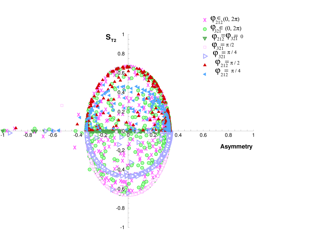
Figure 1: Transverse polarization of the electron in $\mu^{+}\to e^{+}e^{-}e^{+}$ versus the P-odd asymmetry $\mathcal{A}$ defined in Eq. (11). The input values for masses correspond to the ones at the $\alpha$ benchmark in [15] with $m_{\tilde{\nu}_{\mu}}\simeq m_{\tilde{\nu}_{\tau}}\simeq 285$ GeV. Random values between $10^{-5}$ up to bounds in Table 1 are assigned to the $\lambda$ couplings and points at which ${\rm Br}(\mu\to eee)\in 5\cdot 10^{-13}(1\pm 10\%)$ are selected. To calculate $\langle s_{\hat{T}_{2}}\rangle$ and $\mathcal{A}$, we have set $\mathbb{P}_{\mu}=100\%$ and $\theta=\pi/2$ (see definitions in Eqs. (12,13)). $\varphi_{ijk}$ is the phase of $\lambda_{ijk}$. Points with different colors and symbols correspond to a nonzero value for $\varphi_{ijk}$ as described in the legend. For each set, the rest of phases vanish. For points shown by $\times$ and $\circ$, the corresponding phase takes random values at a linear scale from ($0,2\pi$).

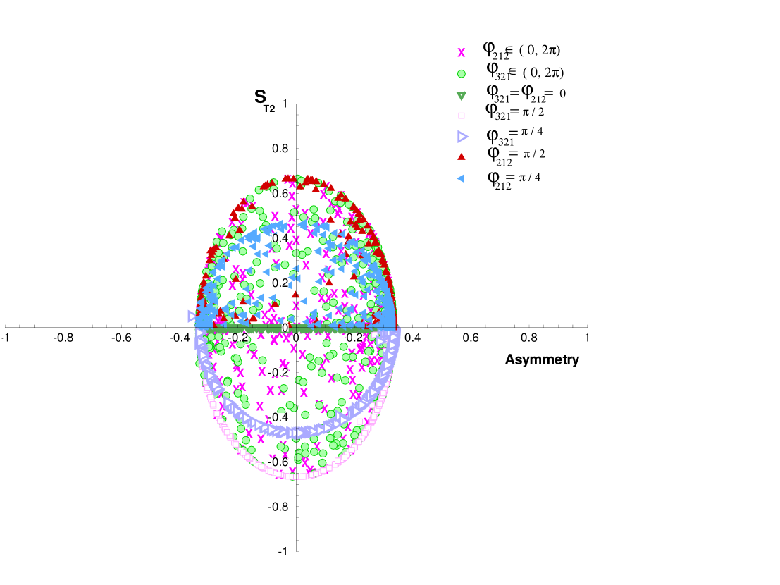
Figure 2: The same as Fig. 1, except that we have removed the points at which $8|G_{1}|^{2}/(|B_{1}|^{2}+|B_{2}|^{2})>0.05$.

Let us suppose ${\rm Br}(\mu\to eee)$ is measured and found to be close to $10^{-12}$. Let us moreover suppose that the Dalitz plots reveal that $B_{1}$ and $B_{2}$ give the dominant contribution to this decay as it is expected in the case that LFV effects originate from $\lambda_{ijk}$. If the MEG experiment at PSI reports a null result (i.e., ${\rm Br}(\mu\to e\gamma)<10^{-13}\$), within the context of MSSM (to be tested at the LHC), such a set of conditions attests our assumption that $\lambda_{ijk}$ is the prime source for LFV. If MEG also finds a signal for $\mu\to e\gamma$, other LFV terms, such as slepton masses or the trilinear soft supersymmetry breaking terms, might contribute to Br$(\mu\to e\gamma)$ but as we discussed earlier, even in this case, we can neglect the contribution from $A_{L}$ and $A_{R}$ to Br($\mu\to eee)$. LFV terms in slepton masses or the trilinear soft supersymmetry breaking terms can contribute to other effective couplings in (1) but the effect will be loop suppressed and negligible. Notice that although within the model under our study, $G_{1}$ and $A_{R}$ are given by the same combinations of $\lambda_{ijk}$, $G_{1}$ is enhanced by a factor of $\log(m_{\tilde{\nu}}^{2}/m_{l}^{2})$ so we do not neglect its contribution [see Eq. (10)]. Neglecting the effects of $A_{R}$, the formulas for $\mathcal{A}$, $\langle s_{\hat{T}^{-}_{1}}\rangle$ and $\langle s_{\hat{T}^{-}_{2}}\rangle$ will have forms:

$$\mathcal{A}={|B_{2}|^{2}-|B_{1}|^{2}-24|G_{1}|^{2}\over 3(|B_{1}|^{2}+|B_{2}|^{2}+8|G_{1}|^{2})}\mathbb{P}_{\mu}\$$ (14)

and

$$\langle s_{\hat{T}_{1}^{-}}\rangle ={4{\Re}[B_{1}B_{2}^{*}]\mathbb{P}_{\mu}\sin\theta\over|B_{1}|^{2}(3-\mathbb{P}_{\mu}\cos\theta)+|B_{2}|^{2}(3+\mathbb{P}_{\mu}\cos\theta)+24|G_{1}|^{2}(1-\mathbb{P}_{\mu}\cos\theta)},$$ (15a)

$$\langle s_{\hat{T}_{2}^{-}}\rangle ={4{\Im}[B_{1}B_{2}^{*}]\mathbb{P}_{\mu}\sin\theta\over|B_{1}|^{2}(3-\mathbb{P}_{\mu}\cos\theta)+|B_{2}|^{2}(3+\mathbb{P}_{\mu}\cos\theta)+24|G_{1}|^{2}(1-\mathbb{P}_{\mu}\cos\theta)}\ ,$$ (15b)

in which $\mathbb{P}_{\mu}$ is the polarization of the initial muons.

Moreover the longitudinal polarization is given by

$$\langle s_{\hat{T}_{3}^{-}}\rangle={|B_{1}|^{2}-|B_{2}|^{2}+8|G_{1}|^{2}-\mathbb{P}_{\mu}\cos\theta\left[(|B_{1}|^{2}+|B_{2}|^{2})/3+8|G_{1}|^{2}\right]\over|B_{1}|^{2}+|B_{2}|^{2}+8|G_{1}|^{2}+\mathbb{P}_{\mu}\cos\theta\left[(|B_{2}|^{2}-|B_{1}|^{2})/3-8|G_{1}|^{2}\right]}\ .$$

Notice when the electron is emitted in the direction perpendicular to the spin of the muon, the transverse polarization is maximal. In our analysis, we will set $\theta=\pi/2$ which experimentally means we study the data from the polarimeter collecting electrons with momentum perpendicular to $\vec{s}_{\mu}$. If more than a single polarimeter is installed, more data can of course be collected. The average polarization can be defined as

$$\overline{\langle s_{\hat{T}_{i}^{-}}\rangle}\equiv{\int_{-1}^{1}\langle s_{\hat{T}_{i}^{-}}\rangle\leavevmode\nobreak\ [d\Gamma(\mu\to eee)/d\cos\theta]\leavevmode\nobreak\ d\cos\theta\over\int_{-1}^{1}[d\Gamma(\mu\to eee)/d\cos\theta]\leavevmode\nobreak\ d\cos\theta}.$$ (16)

For $i=1,2$, $\overline{\langle s_{\hat{T}_{i}^{-}}\rangle}=\frac{\pi}{4}\mathbb{P}_{\mu}\langle s_{\hat{T}_{i}^{-}}\rangle|_{\theta=\frac{\pi}{2}}.$ It is noteworthy that if the values of Br$(\mu\to eee)$, $\mathcal{A}$ and $\langle s_{\hat{T}^{-}_{3}}\rangle|_{\theta=\frac{\pi}{2}}$ are measured, the numerical values of $|B_{1}|$, $|B_{2}|$ and $|G_{1}|$ can be derived.

5 Feasibility of measuring the transverse polarization

The typical experimental setups devoted to the study of muon decay (such as the MEG experiment or the experiment at TRIUMF described in [13]) can be summarized as follows. A proton beam collides on a target producing pions. Charged pions are stopped in the target and decay at rest into a neutrino and a muon. Muons at production are 100 % polarized up to negligible correction due to the neutrino mass [13]. Muons exit the first target and are transmitted to a second target where they stop and then decay at rest. Based on the setup of the experiment, muons of either positive or negative sign can be selected to be transmitted to the second target. Negative muons would form bound states with atoms in the second target so we focus on the decay of positive muons which decay as free states. When muons decay, they are still highly polarized. The degree of depolarization from the production to decay depends on the setup of experiment. Especially if only the muons produced at the surface of the first target are collected (as it is done both in MEG [12] and in the experiment described in [13]), the depolarization will be quite negligible. For example, in the TRIUMF experiment described in [13], the polarization remains above 99% until the muon decay in the second target. For the purpose of the present analysis we can safely replace $\mathbb{P}_{\mu}=100\%$. Notice that unlike the case of [13], even a moderate accuracy in knowledge of $\mathbb{P}_{\mu}$ will be sufficient to perform the present analysis so from this aspect, it is easier to carry out the present measurement [13].

Let us now discuss the possibility of measuring the transverse polarization of the electron in $\mu^{+}\to e^{+}e^{-}e^{+}$. First, let us recall the measurement of the transverse polarization of the positron in $\mu^{+}\to e^{+}\nu_{e}\bar{\nu}_{\mu}$ which was carried out about 25 years ago to extract the Michel parameters [14]. The outline of the polarization measurement is as follows. The emitted positrons interact with electrons in a target which are polarized in a direction perpendicular to the momentum of the emitted positrons by a magnetic field. The electron positron pair annihilate into a photon pair. By studying the azimuthal distribution of the final photon pairs, the transverse polarization of the emitted positron can be determined. In our case, we are interested in measuring the transverse polarization of the final electron rather than the final positron. Fortunately, a similar setup can be employed to determine the transverse polarization of the emitted electron. Of course in this case instead of annihilation into a photon pair, the Möller scattering ($e_{1}^{-}e_{2}^{-}\to e_{3}^{-}e_{4}^{-}$) will take place. Similar to the case of $e^{-}e^{+}\to\gamma\gamma$, the azimuthal distribution of the final particles carry information on the spin of the emitted electron. Let us take the $\hat{z}$ direction to be parallel to the momentum of the emitted electron (the momentum of $e_{1}^{-}$) and take $\hat{x}$ to be in the direction of the spin of the electron at rest in the magnetized target (i.e., the spin of $e_{2}^{-}$):

$$P_{1}=(\sqrt{k^{2}+m_{e}^{2}},0,0,k)\ \ \ {\rm and}\ \ \ P_{2}=(m_{e},0,0,0)\ .$$

The spin of $e_{1}$ can be described by $(a\ b)$ where $|a|^{2}+|b|^{2}=1$:

$$\langle s_{x}\rangle=2\Re[ba^{*}],\ \langle s_{y}\rangle=2\Im[ba^{*}]\ {\rm and}\ \langle s_{z}\rangle=|a|^{2}-|b|^{2}\ .$$

The angular distribution of the final particles are described by $(\theta,\phi)$:

$$P_{3}=(\sqrt{k^{\prime 2}+m_{e}^{2}},k^{\prime}\sin\theta\cos\phi,k^{\prime}\sin\theta\sin\phi,k^{\prime}\cos\theta)\ {\rm and}\ P_{4}=P_{1}+P_{2}-P_{3}\ ,$$

where the energy-momentum conservation implies

$$k^{\prime}={m_{e}k\over m_{e}+k(1-\cos\theta)}\ .$$

A cumbersome but straightforward calculation shows that

$$\int_{0}^{2\pi}\frac{d\sigma}{d\cos\theta\leavevmode\nobreak\ d\phi}\cos\phi d\phi=$$ (17)

$$(|b|^{2}-|a|^{2}){k^{\prime 4}e^{4}(1-\cos\theta)\sin\theta\over 64\pi m_{e}^{4}(k-k^{\prime})}\left({k^{\prime}(1-\cos\theta)\over(k-k^{\prime})^{2}}+{k^{\prime}(1-\cos\theta)-m_{e}\over(k-m_{e})^{2}}-{m_{e}(1-2k^{\prime}\cos\theta/k)\over(k-k^{\prime})(k-m_{e})}\right)$$

and

$$\int_{0}^{2\pi}\frac{d\sigma}{d\cos\theta\leavevmode\nobreak\ d\phi}\sin 2\phi d\phi=$$ (18)

$$\Im[ab^{*}]{k^{\prime 5}e^{4}(1-\cos\theta)\sin^{2}\theta\over 64\pi m_{e}^{4}(k-k^{\prime})}\left({m_{e}/k\over(k-k^{\prime})^{2}}+{m_{e}/k\over(k-m_{e})^{2}}-{1\over(k-k^{\prime})(k-m_{e})}\right)\ .$$

Thus, by measuring the partial cross section, $d\sigma/(d\cos\theta\leavevmode\nobreak\ d\phi)$, and taking the above integrals, $a$ and $b$ (up to an overall phase) can be determined and the spin of $e_{1}$ can be therefore reconstructed.

There are two problems that complicate the measurement: (1) In the lab frame where $e^{-}_{2}$ is at rest, the majority of the electrons are scattered in the forward direction within a narrow cone with opening angle of $O(2m_{e}/k)$ where $k\sim m_{\mu}/3\sim 30\leavevmode\nobreak\ {\rm MeV}$. The same problem existed in the case of measuring the polarization of the emitted positron. (2) The scattered electron $e_{3}$ can again scatter on the electrons in the magnetized target before exiting it. Multiple scattering will distort the azimuthal distribution in which the information of the spin of the initial electron is imprinted. The same problem existed is the case of measuring the spin of the positron as the photons produced in the electron positron annihilation could Compton scatter on the electrons in the magnetized target. In both cases, the total scattering cross section is of order of $e^{4}/(16\pi m_{e}k)$. Fortunately, there are established techniques to overcome these difficulties.

6 Combined analysis of $\mathcal{A}$ and $\langle s_{\hat{T}_{2}^{-}}\rangle$

By rephasing the leptonic fields, three out of nine phases in the $\lambda$ couplings can be absorbed. Let us consider the basis in which $\lambda_{311}$, $\lambda_{211}$ and $\lambda_{312}$ are all real. The rest of $\lambda$’s in this basis can in general be complex among which the phases of $\lambda_{321}$, $\lambda_{212}$, $\lambda_{322}$ and $\lambda_{323}$ can lead to a nonzero $\langle s_{\hat{T}^{-}_{2}}\rangle$. We first concentrate on the phases of $\lambda_{321}$ and $\lambda_{212}$ which contribute to $B_{1}$ at a tree level. We then comment on the rest of phases. As we discussed in the previous section, we can safely replace $\mathbb{P}_{\mu}=100\leavevmode\nobreak\ \%$ and that is what we do in the following. For any given polarization, our results can be simply rescaled.

Figs. 1 and 2 demonstrate the dependence of $\langle s_{\hat{T}^{-}_{2}}\rangle$ and $\mathcal{A}$ on the phases. To draw these scatter plots, we have assigned random numbers at a logarithmic scale from $10^{-5}$ to the upper bound on $|\lambda|$’s. ($|\lambda|$’s take up random values in a logarithmic scale.) As explained in the caption, various values are assigned to the phase of either $\lambda_{321}$ or $\lambda_{212}$, setting the other one (as well as the rest of phases) equal to zero. The phase of $\lambda_{ijk}$ is denoted by $\varphi_{ijk}$. We have selected the configurations of $\lambda$ for which Br$(\mu\to eee)$ lies within the range Br$(\mu\to eee)=5\times 10^{-13}(1\pm 10\%)$. From an experimental perspective, this means that we have supposed Br$(\mu\to eee)$ is measured to be in the range $5\times 10^{-13}(1\pm 10\%)$. The 10% uncertainty is a nominal value that we have taken as an example to highlight the fact that the branching ratio measurement will suffer from a finite uncertainty. Our results are robust against varying the value of this uncertainty. In fact by rescaling the coupling by a $\delta N$ percent, Br$(\mu\to eee)$ will change by $4\delta N\%$ but $\langle s_{\hat{T}_{2}^{-}}\rangle$ and $\mathcal{A}$, being ratios, will not vary.

Points denoted by pink crosses are the points at which $\varphi_{321}=0$ and $\varphi_{212}$ takes up random values in $(0,2\pi)$. On the contrary, those shown by green circles correspond to the cases that $\varphi_{212}=0$ and $\varphi_{321}$ takes random values in the range $(0,2\pi)$. As seen from the figures, the areas over which pink $\times$ and green $\circ$ are scattered completely overlap which means if $|\lambda|$’s are unknown, the two solutions are indistinguishable. However, valuable information from $\langle s_{\hat{T}_{2}^{-}}\rangle$ can be derived. For example if both CP-violating phases vanish, $\langle s_{\hat{T}_{2}^{-}}\rangle$ also vanishes (points indicated by green $\nabla$).

Remember that, while $B_{1}$ and $B_{2}$ receive nonzero contributions at a tree level, $G_{1}$ receives a contribution only at a loop level. As long as $G_{1}$ has a negligible value, for given $\mathcal{A}$ and Br($\mu\to eee)$, $|B_{1}|$ and $|B_{2}|$ are fixed. It is straightforward to check that, for $|G_{1}|\to 0$,

$$|\mathcal{A}|<\frac{1}{3}\ \ \ {\rm and}\ \ \ |\langle s_{\hat{T}_{2}^{-}}\rangle|<\frac{2}{3}\sqrt{1-9\mathcal{A}^{2}}\ .$$ (19)

As seen in the figures, the majority of points lie inside an oval-shaped region whose boundaries are given by Eq. (19). These are the points for which the contribution from loop suppressed $|G_{1}|^{2}$ can be neglected. As seen from Fig. 1, there are only few points (about 2 percent of all points) lying outside the oval-shaped region. At points with $\mathcal{A}<-1/3$, the contribution from $|G_{1}|^{2}$ dominates. For $\mathcal{A}<-0.5$, we find $|\langle s_{\hat{T}_{1}^{-}}\rangle|,|\langle s_{\hat{T}_{2}^{-}}\rangle|\ll 0.1$ which is expected from Eqs. (14) and (15). In Fig. 2, we have removed the points for which $8|G_{1}|^{2}/(|B_{1}|^{2}+|B_{2}|^{2})>0.05$. As a result, Fig. 2 does not include points outside the oval-shaped region. If the pair $(\mathcal{A},\langle s_{\hat{T}_{2}^{-}}\rangle$) turns out to be outside the oval-shaped region, it means $|G_{1}|$ is relatively large. This can happen if $\lambda_{322}$ is more than 50 times larger than the rest of $\lambda_{ijk}$ (see Eqs. (10) and table 1) so $\mathcal{A}<-1/3$ indicates that the flavor structure of the $\lambda_{ijk}$ coupling should be hierarchical.

As mentioned above, in the limit $G_{1}\to 0$, for a given $\mathcal{A}$ and $Br(\mu\to eee)$, $|B_{1}|$ and $|B_{2}|$ are fixed so $\langle s_{\hat{T}_{2}^{-}}\rangle$ determines $\arg[B_{2}B_{1}^{*}]$. Thus, if all the phases except $\varphi_{321}$ are zero, $\langle s_{\hat{T}_{2}^{-}}\rangle$ will determine $\varphi_{321}$. This can be seen in Fig. 2. That is impressive that $\varphi_{321}$ can be derived even without knowledge of $|\lambda_{ijk}|$’s (of course under the assumption of a single nonzero phase). Deriving the value of $\varphi_{212}$ is going to be more challenging even when we set all the other phases equal to zero. As seen from Figs. 1 and 2, for a given $\mathcal{A}$ and a certain value of $\varphi_{212}$, depending on the configuration of the absolute values of the $\lambda$’s, $\langle s_{\hat{T}_{2}^{-}}\rangle$ can take any value between zero and its maximal value which is $(2/3)(1-9\mathcal{A})^{1/2}\sin\varphi_{212}$. This is understandable as $B_{2}$ receives contributions from various terms (compare Eqs. (10b) and (10c)) so unlike the case of ($\varphi_{212}=0$, $\varphi_{321}\neq 0$), in this case, the nonzero phase is not given by $\arg[B_{1}B_{2}^{*}]$.

From Fig. 2, we observe that for $|\mathcal{A}|<0.2$, by simultaneous measurements of $\mathcal{A}$ and $\langle s_{\hat{T}_{2}^{-}}\rangle$ with reasonable accuracy, even without independent knowledge of $|\lambda_{ijk}|$, solutions with ($\varphi_{321}=\pi/2$,$\varphi_{212}=0$) and ($\varphi_{321}=\pi/4$,$\varphi_{212}=0$) can be distinguished (see points denoted by violet $\triangleright$ and pink $\square$). Notice that all points denoted by red $\vartriangle$ and blue $\triangleleft$ corresponding respectively to ($\varphi_{321}=0$,$\varphi_{212}=\pi/2$) and ($\varphi_{321}=0$,$\varphi_{212}=\pi/4$) lie above the horizontal axis. Solutions with positive and negative $\sin\varphi_{212}$ are distinguishable but deriving the value of $\varphi_{212}$ without knowledge of $|\lambda_{ijk}|$ does not seem to be practical. We have found that the contributions from the phases that enter only at loop level (i.e., $\varphi_{322}$, $\varphi_{313}$ and $\varphi_{323}$) to $\langle s_{\hat{T}^{-}_{2}}\rangle$ are smaller than $0.1$. Thus, in deriving the values of $\varphi_{212}$ and $\varphi_{321}$ from $\langle s_{\hat{T}_{2}^{-}}\rangle$, the potential contributions from the rest of the phases can be ignored.

As discussed above, an upper bound on $|G_{1}|$ can considerably simplify the analysis and solve the degeneracies. Although $|G_{1}|^{2}$ (more precisely, $|G_{1}|^{2}+|C_{2}|^{2}/16$) can in principle be extracted from the energy distribution of final particles, within the present model, its value will most probably be too small to be measured so in practice only an upper bound on $|G_{1}|$ can be extracted as we have assumed in deriving Fig. 2. Notice that

$$\lim_{\leavevmode\nobreak\ \leavevmode\nobreak\ \leavevmode\nobreak\ \leavevmode\nobreak\ |G_{1}|\to 0}\ \frac{\langle s_{\hat{T}_{3}^{-}}\rangle|_{\theta=\frac{\pi}{2}}}{\mathcal{A}}=3\ .$$

That is while if $G_{1}$ and $G_{2}$ (or $C_{1}$ and $C_{2}$) gave the main contribution to $\mu\to eee$, we would expect that $\langle s_{\hat{T}_{3}^{-}}\rangle|_{\theta=\frac{\pi}{2}}/\mathcal{A}=1$. The ratio of longitudinal polarization to $\mathcal{A}$ can therefore be regarded as a cross-check for the smallness of $|G_{1}|$.

To draw Figs 1 and 2, we have used the spectrum at the $\alpha$ benchmark [15] as the input: i.e., We have set $m_{\tilde{\nu}_{\mu}}=m_{\tilde{\nu}_{\tau}}=285\leavevmode\nobreak\ {\rm GeV}$. For two reasons, we expect the results to be robust against varying the input masses: (i) Varying $m_{\tilde{\nu}_{\mu}}^{2}$ and $m_{\tilde{\nu}_{\tau}}^{2}$ is respectively equivalent to rescaling $\lambda_{211}$ and $\lambda_{311}$ (see Eqs. (10b) and (10c)). (ii) Both $\mathcal{A}$ and $\langle s_{\hat{T}_{2}^{-}}\rangle$ are defined as ratios so the dependence on the supersymmetry scale disappears. We have re-drawn the diagram for different benchmarks. As expected, the results are not sensitive to the input for the mass spectrum.

It is noteworthy that if the only sources of LFV are the $\lambda_{ijk}$’s giving rise to Br$(\mu\to eee)$, Br$(\mu\to e\gamma)$ will be smaller than $10^{-13}$ so if the MEG experiment reports a $\mu\to e\gamma$ signal, sources for $\mu\to e\gamma$ other than $\lambda_{ijk}$’s must exist.

As seen in Figs. 1 and 2, both $\mathcal{A}$ and $\langle s_{\hat{T}_{2}^{-}}\rangle$ can be relatively large so as long as the errors in their measurement (i.e., $\delta\mathcal{A}$ and $\delta\langle s_{\hat{T}_{2}^{-}}\rangle$) are below $\sim 0.1$, their nonzero values can be established. Suppose the numbers of electrons studied to derive $\mathcal{A}$ and $\langle s_{\hat{T}_{2}^{-}}\rangle$ are respectively $\mathcal{N}_{A}$ and $\mathcal{N}_{s}$. We roughly expect the statistical errors to be $\delta\mathcal{A}\sim 1/\sqrt{\mathcal{N}_{A}}$ and $\delta\langle s_{\hat{T}_{2}^{-}}\rangle\sim 1/\sqrt{\mathcal{N}_{s}}$. To derive $\mathcal{A}$, the majority of the emitted electrons can in principle be employed, so with a few hundred $\mu^{+}\to e^{+}e^{-}e^{+}$ decays, the statistical error in the measurement of $\mathcal{A}$ will be reasonably small and below 0.1. However, we expect only a fraction of the emitted electrons, $r$, to enter the polarimeters so for establishing nonzero $\langle s_{\hat{T}_{2}^{-}}\rangle$, the total number of $\mu^{+}\to e^{+}e^{-}e^{+}$ decays has to be larger than $100/r$. That is if $r\sim 10\%$, the total number of $\mu^{+}\to e^{+}e^{-}e^{+}$ has to be larger than a few thousand.

In the above analysis, we have employed information on the $R$-parity violating couplings from only the LFV rare decays. The R-parity violating couplings can in principle be directly measured by accelerators. $|\lambda_{i11}|$ leads to a resonant production of $\tilde{\nu}_{i}$ in a $e^{-}e^{+}$ collider ($e^{-}e^{+}\to\tilde{\nu}_{i}$) so $|\lambda_{i11}|$ can be derived provided that $|\lambda_{i11}|>10^{-5}$ and the center of mass energy is equal to the mass of $\tilde{\nu}_{i}$ [16, 10]. Moreover, the $\lambda$ couplings can lead to $\tilde{\nu}_{i}\to l_{j}^{+}l_{i}^{-}$, $\tilde{\chi}_{1}^{0}\to\bar{\nu}_{i}l_{j}^{+}l_{k}^{-}$ and $\tilde{\chi}_{1}^{+}\to\nu_{k}\bar{\nu}_{i}l_{j}^{+},l_{i}^{+}l_{k}^{+}l_{j}^{-}$ [17, 10] where $\tilde{\chi}_{1}^{0}$ and $\tilde{\chi}_{1}^{+}$ are the lightest neutralino and chargino. Thus, by measuring the decay length and the flavor of the final charged leptons, $|\lambda_{ijk}|$ can in principle be extracted. If $|\lambda_{ijk}|<\mathcal{O}(10^{-5})$, the decay length will be too small to be resolved [10]. This method is therefore sensitive only to the values of $|\lambda_{ijk}|$ smaller than $\mathcal{O}(10^{-5})$. If $|\lambda|$’s are all smaller than $10^{-5}$, each $|\lambda_{ijk}|$ might be extracted from $\tilde{\nu}_{i}\to l_{j}^{+}l_{i}^{-}$, $\tilde{\chi}_{1}^{0}\to\bar{\nu}_{i}l_{j}^{+}l_{k}^{-}$ and $\tilde{\chi}_{1}^{+}\to\nu_{k}\bar{\nu}_{i}l_{j}^{+},l_{i}^{+}l_{k}^{+}l_{j}^{-}$ but in this case $Br(\mu\to eee)$ will be too small ($Br(\mu\to eee)<10^{-16}$). Let us now consider the range, $m_{susy}\sim 100$ GeV, $\lambda_{211},\lambda_{311}>10^{-3}$ and $\lambda_{ijk}\sim 10^{-5}$ with $ijk\neq 211,311$. In this range, $e^{-}e^{+}\to\tilde{\nu}_{i}$ yields $|\lambda_{i11}|$ and Br$(\mu\to eee)$ is close to the present bound. Moreover, for $ijk\neq 211,311$, $\tilde{\nu}_{i}\to l_{j}^{+}l_{k}^{-}$ and $\tilde{\chi}_{1}^{0}\to\bar{\nu}_{i}l_{j}^{+}l_{k}^{-}$ will have a resolvable decay length but the point is that the decay modes involving $\lambda_{211}$ and $\lambda_{311}$ will dominate and lead to a decay length too short to be observable: e.g., $\Gamma(\tilde{\nu}_{\mu}\to e^{+}e^{-})/\Gamma(\tilde{\nu}_{\mu}\to\tau^{+}\tau^{-})\sim{10^{4}}$. Thus, even in case that the $R$-parity conserving decay modes are kinematically forbidden, extracting the decay lengths will be quite challenging. Let us however suppose that these experimental difficulties are partly solved and certain $|\lambda_{ijk}|$ (but not necessarily all) are measured. Such achievement might not be out of reach if $\lambda_{i11}\sim 10^{-4}$ and the rest of $\lambda$’s are of order of $10^{-5}$. Complementary information can then be derived from Br($\mu\to eee$), $\mathcal{A}$ and $\langle s_{T_{2}^{-}}\rangle$: Neglecting the $|G_{1}|^{2}$ effects, Br($\mu\to eee$) and $\mathcal{A}$ give $|B_{1}|$ and $|B_{2}|$ which to leading order correspond to $|\lambda_{311}|\cdot|\lambda_{321}|$ and $|\lambda_{211}^{*}\lambda_{212}+(m_{\tilde{\nu}_{\mu}}^{2}/m_{\tilde{\nu}_{\mu}}^{2})\lambda_{311}^{*}\lambda_{312}|$, respectively. Thus, if $\lambda_{311}$ is extracted from $e^{+}e^{-}\to\tilde{\nu}_{\tau}$ at ILC, the measurement of Br($\mu\to eee$) and $\mathcal{A}$ gives $|\lambda_{321}|$. If $|\lambda_{211}|$, $|\lambda_{212}|$, $|\lambda_{311}|$ and $|\lambda_{312}|$ are all derived by accelerators, this method will give the phase of $\lambda_{212}$. The measurement of $\langle s_{\hat{T}_{2}^{-}}\rangle$ will then yield the phase of $\lambda_{321}$.

7 Conclusions and discussion

The trilinear $R$-parity violating Yukawa couplings, $\lambda_{ijk}\hat{L}_{i}\hat{L}_{j}\hat{E}_{k}/2$ can lead to $\mu\to eee$. In particular, $\lambda_{321}$, $\lambda_{311}$, $\lambda_{211}$, $\lambda_{312}$ and $\lambda_{212}$ contribute to $\mu\to eee$ at tree level. By rephasing the lepton fields, we can go to a basis in which $\lambda_{311}$, $\lambda_{312}$ and $\lambda_{211}$ are real. This exhausts the freedom to rephase the other fields so $\lambda_{321}$ and $\lambda_{212}$ can in general be complex and can be considered as sources for CP-violation. Their phases can induce transverse polarization for $e^{-}$ in the direction $\hat{T}_{2}^{-}=\vec{s}_{\mu}\times\vec{P}_{e^{-}}/|\vec{s}_{\mu}\times\vec{P}_{e^{-}}|$. Thus, by measuring this polarization, one can derive information on the CP-violating phases. We have shown that for maximal CP-violation, $|\langle s_{\hat{T}_{2}^{-}}\rangle|$ can reach 2/3 so with a moderate sensitivity to $\langle s_{\hat{T}_{2}^{-}}\rangle$, CP-violation can be established. The sign of the CP-violating phase can also be determined by measuring the sign of $\langle s_{\hat{T}_{2}^{-}}\rangle$.

We have also studied the $P$-odd asymmetry, $\mathcal{A}$ defined in Eq. (11) and discussed the information that from a combined analysis of $\mathcal{A}$ and $\langle s_{\hat{T}_{2}^{-}}\rangle$ can be obtained. For the majority of the $\lambda$ configurations, the tree level effects dominate so the effective coupling $|G_{1}|$ is much smaller than $|B_{1}|$ and $|B_{2}|$ and its effects can therefore be neglected. In this case, $|G_{1}|$ will be too small to be measured but an upper bound can be put on $|G_{1}|$ by studying the energy distribution of the final particles in $\mu\to eee$ or as discussed in the present paper by combining information on $\mathcal{A}$, Br($\mu\to eee$) and $\langle s_{\hat{T}_{3}^{-}}\rangle$. We have noticed that if $8|G_{1}|^{2}<0.05(|B_{1}|^{2}+|B_{2}|^{2})$, the analysis becomes much simpler because of two reasons: (i) The contributions of the phases of $\lambda_{322}$, $\lambda_{323}$ and $\lambda_{313}$ to $\langle s_{\hat{T}_{2}^{-}}\rangle$ can be neglected. These are the couplings that contribute only at a loop level. (ii) For given $\mathcal{A}$ and Br($\mu\to eee$), the absolute values of $B_{1}$ and $B_{2}$ are fixed which simplifies the analysis. In particular, restricting the analysis to a single CP-violating phase, the simultaneous measurement of $\mathcal{A}$ and $\langle s_{\hat{T}_{2}^{-}}\rangle$ yields the phase of $\lambda_{321}$ even if the values of $|\lambda_{ijk}|$ are not a priori known. Degeneracies however exist between solutions for which the phases of $\lambda_{212}$ and $\lambda_{321}$ are both nonzero. By measuring $\mathcal{A}$ and $\langle s_{\hat{T}_{2}^{-}}\rangle$, different classes of solutions can be distinguished. If the absolute values of $\lambda$ are measured by an accelerator-based experiment (or by some other methods), the measurements in $\mu\to eee$ can yield both phases. In fact, if the tree level contribution dominates, the relevant $\lambda$ parameters can be over-constrained.

Neglecting the contribution of $|G_{1}|$, we find $-1/3<\mathcal{A}<1/3$ and $-2\sqrt{(1-9\mathcal{A}^{2})/9}<\langle s_{\hat{T}_{2}^{-}}\rangle<2\sqrt{(1-9\mathcal{A}^{2})/9}$. Only at a small fraction of the parameter space where ($\lambda_{322}\gg$ rest of $\lambda$), the loop effects can dominate and lead to $\mathcal{A}<-1/3$. Within the model under consideration, $\mathcal{A}<-1/3$ therefore indicates a hierarchical flavor structure for the $\lambda$ parameters.

Stopped $\mu^{-}$ would form bound states with the atoms before they decay. Because of this technical difficulty, we have concentrated on the decay of $\mu^{+}$ and the spin of the final electron emitted from it. Similar consideration holds for the positron in free decay of negative muon; i.e., for $e^{+}$ in $\mu^{-}\to e^{-}e^{+}e^{-}$. Within the present model, the transverse polarizations of the electrons in $\mu^{-}\to e^{-}e^{+}e^{-}$ (or that of the positrons in $\mu^{+}\to e^{+}e^{-}e^{+}$) are loop-suppressed.

There are established techniques to measure the transverse polarization of the positron based on the azimuthal distribution of the photon pair produced by the annihilation of the positron on the polarized electrons in a thin magnetized target [14]. We have shown that a similar setup can be employed to measure the transverse polarization of the electrons, too. In fact, the azimuthal distribution of the final electrons in Möller scattering, $e_{1}^{-}e_{2}^{-}\to e_{3}^{-}e_{4}^{-}$ with polarized $e_{2}^{-}$ is sensitive to the polarization of $e_{1}^{-}$. The challenges before this measurement are similar to the ones in [14] and can be overcome by similar methods.

One can repeat similar discussion for three body LFV decays of $\tau$ lepton such as $\tau\to\mu\mu\mu$ or $\tau\to eee$. The measurements of the angular distribution and polarization of the final particles in these decays can provide complementary information on the $\lambda_{ijk}$ couplings. Such a study will be presented elsewhere.

References

[1]
C. Amsler et al. [Particle Data Group],
Phys. Lett. B 667 (2008) 1.
[2]
A. de Gouvea, S. Lola and K. Tobe,
Phys. Rev. D 63 (2001) 035004
[arXiv:hep-ph/0008085].
[3]
Y. Farzan,
Phys. Lett. B 677 (2009) 282
[arXiv:0902.2445 [hep-ph]].
[4]
S. Y. Ayazi and Y. Farzan,
JHEP 0901 (2009) 022
[arXiv:0810.4233 [hep-ph]];
Y. Farzan,
Int. J. Mod. Phys. A 24 (2009) 3403.
[5]
Y. Farzan,
JHEP 0707 (2007) 054
[arXiv:hep-ph/0701106].
[6]
A. Masiero and A. Riotto,
Phys. Lett. B 289 (1992) 73
[arXiv:hep-ph/9206212];
Y. Farzan, work in progress.
[7]
Y. Kuno and Y. Okada,
Rev. Mod. Phys. 73 (2001) 151
[arXiv:hep-ph/9909265].
[8]
L. J. Hall and M. Suzuki,
Nucl. Phys. B 231 (1984) 419;
K. S. Babu and R. N. Mohapatra,
Phys. Rev. Lett. 64 (1990) 1705.
[9]
G. Costa, J. R. Ellis, G. L. Fogli, D. V. Nanopoulos and F. Zwirner,
Nucl. Phys. B 297 (1988) 244;
P. Langacker and D. London,
Phys. Rev. D 38 (1988) 886;
V. D. Barger, G. F. Giudice and T. Han,
Phys. Rev. D 40 (1989) 2987.
[10]
R. Barbier et al.,
Phys. Rept. 420 (2005) 1
[arXiv:hep-ph/0406039].
[11]
Y. Kao and T. Takeuchi,
arXiv:0909.0042 [hep-ph].
[12]
http://meg.web.psi.ch/docs/
[13]
B. Jamieson et al.,
Phys. Rev. D 74 (2006) 072007.
[14]
H. Burkard et al.,
Phys. Lett. B 160 (1985) 343.
[15]
A. De Roeck, J. R. Ellis, F. Gianotti, F. Moortgat, K. A. Olive and L. Pape,
Eur. Phys. J. C 49 (2007) 1041
[arXiv:hep-ph/0508198].
[16]
L. Roszkowski,
arXiv:hep-ph/9309208.
[17]
H. K. Dreiner and G. G. Ross,
Nucl. Phys. B 365 (1991) 597;
R. Barbier et al.,
arXiv:hep-ph/9810232.