The Recognition of Tolerance
and Bounded Tolerance Graphs

Abstract.

Tolerance graphs model interval relations in such a way that intervals can tolerate a certain degree of overlap without being in conflict. This subclass of perfect graphs has been extensively studied, due to both its interesting structure and its numerous applications. Several efficient algorithms for optimization problems that are NP-hard on general graphs have been designed for tolerance graphs. In spite of this, the recognition of tolerance graphs – namely, the problem of deciding whether a given graph is a tolerance graph – as well as the recognition of their main subclass of bounded tolerance graphs, have been the most fundamental open problems on this class of graphs (cf. the book on tolerance graphs [14]) since their introduction in 1982 [11]. In this article we prove that both recognition problems are NP-complete, even in the case where the input graph is a trapezoid graph. The presented results are surprising because, on the one hand, most subclasses of perfect graphs admit polynomial recognition algorithms and, on the other hand, bounded tolerance graphs were believed to be efficiently recognizable as they are a natural special case of trapezoid graphs (which can be recognized in polynomial time) and share a very similar structure with them. For our reduction we extend the notion of an acyclic orientation of permutation and trapezoid graphs. Our main tool is a new algorithm that uses vertex splitting to transform a given trapezoid graph into a permutation graph, while preserving this new acyclic orientation property. This method of vertex splitting is of independent interest; very recently, it has been proved a powerful tool also in the design of efficient recognition algorithms for other classes of graphs [21].

1. Introduction

1.1. Tolerance graphs and related graph classes

A simple undirected graph ${G=(V,E)}$ on $n$ vertices is a tolerance graph if there exists a collection ${I=\{I_{i}\ |\ i=1,2,\ldots,n\}}$ of closed intervals on the real line and a set ${t=\{t_{i}\ |\ i=1,2,\ldots,n\}}$ of positive numbers, such that for any two vertices ${v_{i},v_{j}\in V}$, ${v_{i}v_{j}\in E}$ if and only if ${|I_{i}\cap I_{j}|\geq\min\{t_{i},t_{j}\}}$. The pair ${\langle I,t\rangle}$ is called a tolerance representation of $G$. If $G$ has a tolerance representation ${\langle I,t\rangle}$, such that ${t_{i}\leq|I_{i}|}$ for every $i=1,2,\ldots,n$, then $G$ is called a bounded tolerance graph and ${\langle I,t\rangle}$ a bounded tolerance representation of $G$.

Tolerance graphs were introduced in [11], in order to generalize some of the well known applications of interval graphs. The main motivation was in the context of resource allocation and scheduling problems, in which resources, such as rooms and vehicles, can tolerate sharing among users [14]. If we replace in the definition of tolerance graphs the operator min by the operator max, we obtain the class of max-tolerance graphs. Both tolerance and $\max$-tolerance graphs find in a natural way applications in biology and bioinformatics, as in the comparison of DNA sequences from different organisms or individuals [17], by making use of a software tool like BLAST [1]. Tolerance graphs find numerous other applications in constrained-based temporal reasoning, data transmission through networks to efficiently scheduling aircraft and crews, as well as contributing to genetic analysis and studies of the brain [13, 14]. This class of graphs has attracted many research efforts [14, 12, 13, 15, 8, 4, 18, 2, 24, 22], as it generalizes in a natural way both interval graphs (when all tolerances are equal) and permutation graphs (when $t_{i}=|I_{i}|$ for every $i=1,2,\ldots,n$) [11]. For a detailed survey on tolerance graphs we refer to [14].

A comparability graph is a graph which can be transitively oriented. A co-comparability graph is a graph whose complement is a comparability graph. A trapezoid (resp. parallelogram and permutation) graph is the intersection graph of trapezoids (resp. parallelograms and line segments) between two parallel lines $L_{1}$ and $L_{2}$ [10]. Such a representation with trapezoids (resp. parallelograms and line segments) is called a trapezoid (resp. parallelogram and permutation) representation of this graph. A graph is bounded tolerance if and only if it is a parallelogram graph [19, 2]. Permutation graphs are a strict subset of parallelogram graphs [3]. Furthermore, parallelogram graphs are a strict subset of trapezoid graphs [25], and both are subsets of co-comparability graphs [14, 10]. On the contrary, tolerance graphs are not even co-comparability graphs [14, 10]. Recently, we have presented in [22] a natural intersection model for general tolerance graphs, given by parallelepipeds in the three-dimensional space. This representation generalizes the parallelogram representation of bounded tolerance graphs, and has been used to improve the time complexity of minimum coloring, maximum clique, and weighted independent set algorithms on tolerance graphs [22].

Although tolerance and bounded tolerance graphs have been studied extensively, the recognition problems for both these classes have been the most fundamental open problems since their introduction in 1982 [14, 10, 5]. Therefore, all existing algorithms assume that, along with the input tolerance graph, a tolerance representation of it is given. The only result about the complexity of recognizing tolerance and bounded tolerance graphs is that they have a (non-trivial) polynomial sized tolerance representation, hence the problems of recognizing tolerance and bounded tolerance graphs are in the class NP [15]. Recently, a linear time recognition algorithm for the subclass of bipartite tolerance graphs has been presented in [5]. Furthermore, the class of trapezoid graphs (which strictly contains parallelogram, i.e. bounded tolerance, graphs [25]) can be also recognized in polynomial time [20, 26, 21]. On the other hand, the recognition of $\max$-tolerance graphs is known to be NP-hard [17]. Unfortunately, the structure of $\max$-tolerance graphs differs significantly from that of tolerance graphs ($\max$-tolerance graphs are not even perfect, as they can contain induced $C_{5}$’s [17]), so the technique used in [17] does not carry over to tolerance graphs.

Since very few subclasses of perfect graphs are known to be NP-hard to recognize, it was believed that the recognition of tolerance graphs was in P. Furthermore, as bounded tolerance graphs are equivalent to parallelogram graphs [19, 2], which constitute a natural subclass of trapezoid graphs and have a very similar structure, it was plausible that their recognition was also in P.

1.2. Our contribution

In this article, we establish the complexity of recognizing tolerance and bounded tolerance graphs. Namely, we prove that both problems are surprisingly NP-complete, by providing a reduction from the monotone-Not-All-Equal-3-SAT (monotone-NAE-3-SAT) problem. Consider a boolean formula $\phi$ in conjunctive normal form with three literals in every clause (3-CNF), which is monotone, i.e. no variable is negated. The formula $\phi$ is called NAE-satisfiable if there exists a truth assignment of the variables of $\phi$, such that every clause has at least one true variable and one false variable. Given a monotone 3-CNF formula $\phi$, we construct a trapezoid graph $H_{\phi}$, which is parallelogram, i.e. bounded tolerance, if and only if $\phi$ is NAE-satisfiable. Moreover, we prove that the constructed graph $H_{\phi}$ is tolerance if and only if it is bounded tolerance. Thus, since the recognition of tolerance and of bounded tolerance graphs are in the class NP [15], it follows that these problems are both NP-complete. Actually, our results imply that the recognition problems remain NP-complete even if the given graph is trapezoid, since the constructed graph $H_{\phi}$ is trapezoid.

For our reduction we extend the notion of an acyclic orientation of permutation and trapezoid graphs. Our main tool is a new algorithm that transforms a given trapezoid graph into a permutation graph by splitting some specific vertices, while preserving this new acyclic orientation property. One of the main advantages of this algorithm is its robustness, in the sense that the constructed permutation graph does not depend on any particular trapezoid representation of the input graph $G$. Moreover, besides its use in the present paper, this approach based on splitting vertices has been recently proved a powerful tool also in the design of efficient recognition algorithms for other classes of graphs [21].

Organization of the paper. We first present in Section 2 several properties of permutation and trapezoid graphs, as well as the algorithm Split-$U$, which constructs a permutation graph from a trapezoid graph. In Section 3 we present the reduction of the monotone-NAE-3-SAT problem to the recognition of bounded tolerance graphs. In Section 4 we prove that this reduction can be extended to the recognition of general tolerance graphs. Finally, we discuss the presented results and further research directions in Section 5. Some proofs have been omitted due to space limitations; a full version can be found in [23].

2. Trapezoid graphs and representations

In this section we first introduce (in Section 2.1) the notion of an acyclic representation of permutation and of trapezoid graphs. This is followed (in Section 2.2) by some structural properties of trapezoid graphs, which will be used in the sequel for the splitting algorithm Split-$U$. Given a trapezoid graph $G$ and a vertex subset $U$ of $G$ with certain properties, this algorithm constructs a permutation graph $G^{\#}(U)$ with $2|U|$ vertices, which is independent on any particular trapezoid representation of the input graph $G$.

Notation. We consider in this article simple undirected and directed graphs with no loops or multiple edges. In an undirected graph $G$, the edge between vertices $u$ and $v$ is denoted by $uv$, and in this case $u$ and $v$ are said to be adjacent in $G$. If the graph $G$ is directed, we denote by $uv$ the arc from $u$ to $v$. Given a graph ${G=(V,E)}$ and a subset ${S\subseteq V}$, $G[S]$ denotes the induced subgraph of $G$ on the vertices in $S$, and we use $E[S]$ to denote $E(G[S])$. Whenever we deal with a trapezoid (resp. permutation and bounded tolerance, i.e. parallelogram) graph, we will consider w.l.o.g. a trapezoid (resp. permutation and parallelogram) representation, in which all endpoints of the trapezoids (resp. line segments and parallelograms) are distinct [9, 14, 16]. Given a permutation graph $P$ along with a permutation representation $R$, we may not distinguish in the following between a vertex of $P$ and the corresponding line segment in $R$, whenever it is clear from the context. Furthermore, with a slight abuse of notation, we will refer to the line segments of a permutation representation just as lines.

2.1. Acyclic permutation and trapezoid representations

Let $P=(V,E)$ be a permutation graph and $R$ be a permutation representation of $P$. For a vertex $u\in V$, denote by $\theta_{R}(u)$ the angle of the line of $u$ with $L_{2}$ in $R$. The class of permutation graphs is the intersection of comparability and co-comparability graphs [10]. Thus, given a permutation representation $R$ of $P$, we can define two partial orders $(V,<_{R})$ and $(V,\ll_{R})$ on the vertices of $P$ [10]. Namely, for two vertices $u$ and $v$ of $G$, $u<_{R}v$ if and only if $uv\in E$ and $\theta_{R}(u)<\theta_{R}(v)$, while $u\ll_{R}v$ if and only if $uv\notin E$ and $u$ lies to the left of $v$ in $R$. The partial order $(V,<_{R})$ implies a transitive orientation $\Phi_{R}$ of $P$, such that $uv\in\Phi_{R}$ whenever $u<_{R}v$.

Let $G=(V,E)$ be a trapezoid graph, and $R$ be a trapezoid representation of $G$, where for any vertex $u\in V$, the trapezoid corresponding to $u$ in $R$ is denoted by $T_{u}$. Since trapezoid graphs are also co-comparability graphs [10], we can similarly define the partial order $(V,\ll_{R})$ on the vertices of $G$, such that $u\ll_{R}v$ if and only if $uv\notin E$ and $T_{u}$ lies completely to the left of $T_{v}$ in $R$. In this case, we may denote also $T_{u}\ll_{R}T_{v}$.

In a given trapezoid representation $R$ of a trapezoid graph $G$, we denote by $l(T_{u})$ and $r(T_{u})$ the left and the right line of $T_{u}$ in $R$, respectively. Similarly to the case of permutation graphs, we use the relation $\ll_{R}$ for the lines $l(T_{u})$ and $r(T_{u})$, e.g. ${l(T_{u})\ll_{R}r(T_{v})}$ means that the line $l(T_{u})$ lies to the left of the line $r(T_{v})$ in $R$. Moreover, if the trapezoids of all vertices of a subset $S\subseteq V$ lie completely to the left (resp. right) of the trapezoid $T_{u}$ in $R$, we write $R(S)\ll_{R}T_{u}$ (resp. $T_{u}\ll_{R}R(S)$). Note that there are several trapezoid representations of a particular trapezoid graph $G$. Given one such representation $R$, we can obtain another one $R^{\prime}$ by vertical axis flipping of $R$, i.e. $R^{\prime}$ is the mirror image of $R$ along an imaginary line perpendicular to $L_{1}$ and $L_{2}$. Moreover, we can obtain another representation $R^{\prime\prime}$ of $G$ by horizontal axis flipping of $R$, i.e. $R^{\prime\prime}$ is the mirror image of $R$ along an imaginary line parallel to $L_{1}$ and $L_{2}$. We will extensively use these two operations throughout the article.

Definition 2.1.

Let $P$ be a permutation graph with $2n$ vertices $\{u_{1}^{1},u_{1}^{2},u_{2}^{1},u_{2}^{2},\ldots,u_{n}^{1},u_{n}^{2}\}$. Let $R$ be a permutation representation and $\Phi_{R}$ be the corresponding transitive orientation of $P$. The simple directed graph $F_{R}$ is obtained by merging $u_{i}^{1}$ and $u_{i}^{2}$ into a single vertex $u_{i}$, for every $i=1,2,\ldots,n$, where the arc directions of $F_{R}$ are implied by the corresponding directions in $\Phi_{R}$. Then,

1. $R$ is an acyclic permutation representation with respect to $\{u_{i}^{1},u_{i}^{2}\}_{i=1}^{n}$, if $F_{R}$ has no directed cycle,

2. $P$ is an acyclic permutation graph with respect to $\{u_{i}^{1},u_{i}^{2}\}_{i=1}^{n}$, if $P$ has an acyclic representation $R$ with respect to $\{u_{i}^{1},u_{i}^{2}\}_{i=1}^{n}$.

Definition 2.2.

Let $G$ be a trapezoid graph with $n$ vertices and $R$ be a trapezoid representation of $G$. Let $P$ be the permutation graph with $2n$ vertices corresponding to the left and right lines of the trapezoids in $R$, $R_{P}$ be the permutation representation of $P$ induced by $R$, and $\{u_{i}^{1},u_{i}^{2}\}$ be the vertices of $P$ that correspond to the same vertex $u_{i}$ of $G$, $i=1,2,\ldots,n$. Then,

1. $R$ is an acyclic trapezoid representation, if $R_{P}$ is an acyclic permutation representation with respect to $\{u_{i}^{1},u_{i}^{2}\}_{i=1}^{n}$,

2. $G$ is an acyclic trapezoid graph, if it has an acyclic representation $R$.

The following lemma follows easily from Definitions 2.1 and 2.2.

Lemma 2.3.

Any parallelogram graph is an acyclic trapezoid graph.

2.2. Structural properties of trapezoid graphs

In the following, we state some definitions concerning an arbitrary simple undirected graph ${G=(V,E)}$, which are useful for our analysis. Although these definitions apply to any graph, we will use them only for trapezoid graphs. Similar definitions, for the restricted case where the graph $G$ is connected, were studied in [6]. For $u\in V$ and $U\subseteq V$, $N(u)=\{v\in V\ |\ uv\in E\}$ is the set of adjacent vertices of $u$ in $G$, ${N[u]=N(u)\cup\{u\}}$, and ${N(U)=\bigcup_{u\in U}N(u)\setminus U}$. If ${N(U)\subseteq N(W)}$ for two vertex subsets $U$ and $W$, then $U$ is said to be neighborhood dominated by $W$. Clearly, the relationship of neighborhood domination is transitive.

Let ${C_{1},C_{2},\ldots,C_{\omega},\ \omega\geq 1,}$ be the connected components of ${G\setminus N[u]}$ and ${V_{i}=V(C_{i})}$, ${i=1,2,\ldots,\omega}$. For simplicity of the presentation, we will identify in the sequel the component $C_{i}$ and its vertex set $V_{i}$, ${i=1,2,\ldots,\omega}$. For ${i=1,2,\ldots,\omega}$, the neighborhood domination closure of $V_{i}$ with respect to $u$ is the set ${D_{u}(V_{i})=\{V_{p}\ |\ N(V_{p})\subseteq N(V_{i}),\ p=1,2,\ldots,\omega\}}$ of connected components of ${G\setminus N[u]}$. A component $V_{i}$ is called a master component of $u$ if ${|D_{u}(V_{i})|\geq|D_{u}(V_{j})|}$ for all ${j=1,2,\ldots,\omega}$. The closure complement of the neighborhood domination closure ${D_{u}(V_{i})}$ is the set ${D_{u}^{\ast}(V_{i})=\{V_{1},V_{2},\ldots,V_{\omega}\}\setminus D_{u}(V_{i})}$. Finally, for a subset ${S\subseteq\{V_{1},V_{2},\ldots,V_{\omega}\}}$, a component $V_{j}\in S$ is called maximal if there is no component $V_{k}\in S$ such that ${N(V_{j})\subsetneqq N(V_{k})}$.

For example, consider the trapezoid graph $G$ with vertex set $\{u,u_{1},u_{2},u_{3},v_{1},v_{2},v_{3},v_{4}\}$, which is given by the trapezoid representation $R$ of Figure 1. The connected components of ${G\setminus N[u]=\{v_{1},v_{2},v_{3},v_{4}\}}$ are ${V_{1}=\{v_{1}\}}$, ${V_{2}=\{v_{2}\}}$, ${V_{3}=\{v_{3}\}}$, and ${V_{4}=\{v_{4}\}}$. Then, ${N(V_{1})=\{u_{1}\}}$, ${N(V_{2})=\{u_{1},u_{3}\}}$, ${N(V_{3})=\{u_{2},u_{3}\}}$, and ${N(V_{4})=\{u_{3}\}}$. Hence, ${D_{u}(V_{1})=\{V_{1}\}}$, ${D_{u}(V_{2})=\{V_{1},V_{2},V_{4}\}}$, ${D_{u}(V_{3})=\{V_{3},V_{4}\}}$, and ${D_{u}(V_{4})=\{V_{4}\}}$; thus, $V_{2}$ is the only master component of $u$. Furthermore, ${D_{u}^{\ast}(V_{1})=\{V_{2},V_{3},V_{4}\}}$, ${D_{u}^{\ast}(V_{2})=\{V_{3}\}}$, ${D_{u}^{\ast}(V_{3})=\{V_{1},V_{2}\}}$, and ${D_{u}^{\ast}(V_{4})=\{V_{1},V_{2},V_{3}\}}$.

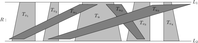
Figure 1. A trapezoid representation $R$ of a trapezoid graph $G$.

Lemma 2.4.

Let $G$ be a simple graph, $u$ be a vertex of $G$, and let $V_{1},V_{2},\ldots,V_{\omega},\ \omega\geq 1$, be the connected components of ${G\setminus N[u]}$. If $V_{i}$ is a master component of $u$, such that ${D_{u}^{\ast}(V_{i})\neq\emptyset}$, then ${D_{u}^{\ast}(V_{j})\neq\emptyset}$ for every component $V_{j}$ of $G\setminus N[u]$.

In the following we investigate several properties of trapezoid graphs, in order to derive the vertex-splitting algorithm Split-$U$ in Section 2.3.

Remark 2.5.

Similar properties of trapezoid graphs have been studied in [6], leading to another vertex-splitting algorithm, called Split-All. However, the algorithm proposed in [6] is incorrect, since it is based on an incorrect property, as was also verified by [7]. In the sequel of this section, we present new definitions and properties. In the cases where a similarity arises with those of [6], we refer to it specifically.

Lemma 2.6.

Let $R$ be a trapezoid representation of a trapezoid graph $G$, and $V_{i}$ be a master component of a vertex $u$ of $G$, such that $R(V_{i}){\ll}_{R}{T_{u}}$. Then, $T_{u}{\ll}_{R}R(V_{j})$ for every component $V_{j}\in D_{u}^{\ast}(V_{i})$.

Definition 2.7.

Let $G$ be a trapezoid graph, $u$ be a vertex of $G$, and $V_{i}$ be an arbitrarily chosen master component of $u$. Then, $\delta_{u}=V_{i}$ and

1. if $D_{u}^{\ast}(V_{i})=\emptyset$, then $\delta_{u}^{\ast}=\emptyset$.

2. if $D_{u}^{\ast}(V_{i})\neq\emptyset$, then $\delta_{u}^{\ast}={V_{j}}$, for an arbitrarily chosen maximal component $V_{j}\in{D_{u}^{\ast}(V_{i})}$.

Actually, as we will show in Lemma 2.10, the arbitrary choice of the components $V_{i}$ and $V_{j}$ in Definition 2.7 does not affect essentially the structural properties of $G$ that we will investigate in the sequel. From now on, whenever we speak about $\delta_{u}$ and $\delta_{u}^{\ast}$, we assume that these arbitrary choices of $V_{i}$ and $V_{j}$ have been already made.

Definition 2.8.

Let $G$ be a trapezoid graph and $u$ be a vertex of $G$. The vertices of $N(u)$ are partitioned into four possibly empty sets:

1. $N_{0}(u)$: vertices not adjacent to either ${\delta_{u}}$ or ${\delta_{u}^{\ast}}$.

2. $N_{1}(u)$: vertices adjacent to ${\delta_{u}}$ but not to ${\delta_{u}^{\ast}}$.

3. $N_{2}(u)$: vertices adjacent to ${\delta_{u}^{\ast}}$ but not to ${\delta_{u}}$.

4. $N_{12}(u)$: vertices adjacent to both ${\delta_{u}}$ and ${\delta_{u}^{\ast}}$.

In the following definition we partition the neighbors of a vertex of a trapezoid graph $G$ into four possibly empty sets. Note that these sets depend on a given trapezoid representation $R$ of $G$, in contrast to the four sets of Definition 2.8 that depend only on the graph $G$ itself.

Definition 2.9.

Let $G$ be a trapezoid graph, $R$ be a representation of $G$, and $u$ be a vertex of $G$. Denote by $D_{1}(u,R)$ and $D_{2}(u,R)$ the sets of trapezoids of $R$ that lie completely to the left and to the right of $T_{u}$ in $R$, respectively. Then, the vertices of $N(u)$ are partitioned into four possibly empty sets:

1. $N_{0}(u,R)$: vertices not adjacent to either $D_{1}(u,R)$ or $D_{2}(u,R)$.

2. $N_{1}(u,R)$: vertices adjacent to $D_{1}(u,R)$ but not to $D_{2}(u,R)$.

3. $N_{2}(u,R)$: vertices adjacent to $D_{2}(u,R)$ but not to $D_{1}(u,R)$.

4. $N_{12}(u,R)$: vertices adjacent to both $D_{1}(u,R)$ and $D_{2}(u,R)$.

Suppose now that $\delta_{u}^{\ast}\neq\emptyset$, and let $V_{i}$ be the master component of $u$ that corresponds to $\delta_{u}$, cf. Definition 2.7. Then, given any trapezoid representation $R$ of $G$, we may assume w.l.o.g. that $R(V_{i}){\ll}_{R}{T_{u}}$, by possibly performing a vertical axis flipping of $R$. The following lemma connects Definitions 2.8 and 2.9; in particular, it states that, if $R(V_{i})\ll_{R}T_{u}$, then the partitions of the set $N(u)$ defined in these definitions coincide. This lemma will enable us to use in the vertex splitting (cf. Definition 2.11) the partition of the set $N(u)$ defined in Definition 2.8, independently of any trapezoid representation $R$ of $G$, and regardless of any particular connected components $V_{i}$ and $V_{j}$ of $G\setminus N[u]$.

Lemma 2.10.

Let $G$ be a trapezoid graph, $R$ be a representation of $G$, and $u$ be a vertex of $G$ with ${\delta_{u}^{\ast}\neq\emptyset}$. Let $V_{i}$ be the master component of $u$ that corresponds to $\delta_{u}$. If ${R(V_{i}){\ll}_{R}{T_{u}}}$, then ${N_{X}(u)=N_{X}(u,R)}$ for every $X\in\{0,1,2,12\}$.

2.3. A splitting algorithm

We define now the splitting of a vertex $u$ of a trapezoid graph $G$, where ${\delta_{u}^{\ast}\neq\emptyset}$. Note that this splitting operation does not depend on any trapezoid representation of $G$. Intuitively, if the graph $G$ was given along with a specific trapezoid representation $R$, this would have meant that we replace the trapezoid $T_{u}$ in $R$ by its two lines $l(T_{u})$ and $r(T_{u})$.

Definition 2.11.

Let $G$ be a trapezoid graph and $u$ be a vertex of $G$, where ${\delta_{u}^{\ast}\neq\emptyset}$. The graph $G^{\#}(u)$ obtained by the vertex splitting of $u$ is defined as follows:

1. $V(G^{\#}(u))=V(G)\setminus\{u\}\cup\{u_{1},u_{2}\}$, where $u_{1}$ and $u_{2}$ are the two new vertices.

2. $E(G^{\#}(u))=E[V(G)\setminus\{u\}]\cup\{u_{1}x\ |\ x\in N_{1}(u)\}\cup\{u_{2}x\ |\ x\in N_{2}(u)\}\cup\{u_{1}x,u_{2}x\ |\ x\in N_{12}(u)\}$.

The vertices $u_{1}$ and $u_{2}$ are the derivatives of vertex $u$.

We state now the notion of a standard trapezoid representation with respect to a particular vertex.

Definition 2.12.

Let $G$ be a trapezoid graph and $u$ be a vertex of $G$, where ${\delta_{u}^{\ast}\neq\emptyset}$. A trapezoid representation $R$ of $G$ is standard with respect to $u$, if the following properties are satisfied:

1. $l(T_{u})\ll_{R}R(N_{0}(u)\cup N_{2}(u))$.

2. $R(N_{0}(u)\cup N_{1}(u))\ll_{R}r(T_{u})$.

Now, given a trapezoid graph $G$ and a vertex subset $U=\{u_{1},u_{2},\ldots,u_{k}\}$, such that $\delta_{u_{i}}^{\ast}\neq\emptyset$ for every $i=1,2,\ldots,k$, Algorithm Split-$U$ returns a graph $G^{\#}(U)$ by splitting every vertex of $U$ exactly once. At every step, Algorithm Split-$U$ splits a vertex of $U$, and finally, it removes all vertices of the set $V(G)\setminus U$, which have not been split.

Algorithm 1 Split-$U$

0:  A trapezoid graph $G$ and a vertex subset $U=\{u_{1},u_{2},\ldots,u_{k}\}$, such that $\delta_{u_{i}}^{*}\neq\emptyset$ for all $i=1,2,\ldots,k$

0:  The permutation graph $G^{\#}(U)$

  $\overline{U}\leftarrow V(G)\setminus U$; $H_{0}\leftarrow G$

  for $i=1$ to $k$ do

     $H_{i}\leftarrow H_{i-1}^{\#}(u_{i})$ {$H_{i}$ is obtained by the vertex splitting of $u_{i}$ in $H_{i-1}$}

  $G^{\#}(U)\leftarrow H_{k}[V(H_{k})\setminus\overline{U}]$ {remove from $H_{k}$ all unsplitted vertices}

  return  $G^{\#}(U)$

Remark 2.13.

As mentioned in Remark 2.5, a similar algorithm, called Split-All, was presented in [6]. We would like to emphasize here the following four differences between the two algorithms. First, that Split-All gets as input a sibling-free graph $G$ (two vertices $u,v$ of a graph $G$ are called siblings, if $N[u]=N[v]$; $G$ is called sibling-free if $G$ has no pair of sibling vertices), while our Algorithm Split-$U$ gets as an input any graph (though, we will use it only for trapezoid graphs), which may contain also pairs of sibling vertices. Second, Split-All splits all the vertices of the input graph, while Split-$U$ splits only a subset of them, which satisfy a special property. Third, the order of vertices that are split by Split-All depends on a certain property (inclusion-minimal neighbor set), while Split-$U$ splits the vertices in an arbitrary order. Last, the main difference between these two algorithms is that they perform a different vertex splitting operation at every step, since Definitions 2.7 and 2.8 do not comply with the corresponding Definitions 4.1 and 4.2 of [6].

Theorem 2.14.

Let $G$ be a trapezoid graph and $U=\{u_{1},u_{2},\ldots,u_{k}\}$ be a vertex subset of $G$, such that $\delta_{u_{i}}^{\ast}\neq\emptyset$ for every $i=1,2,\ldots,k$. Then, the graph $G^{\#}(U)$ obtained by Algorithm Split-$U$, is a permutation graph with $2k$ vertices. Furthermore, if $G$ is acyclic, then $G^{\#}(U)$ is acyclic with respect to $\{u_{i}^{1},u_{i}^{2}\}_{i=1}^{k}$, where $u_{i}^{1}$ and $u_{i}^{2}$ are the derivatives of $u_{i}$, $i=1,2,\ldots,k$.

3. The recognition of bounded tolerance graphs

In this section we provide a reduction from the monotone-Not-All-Equal-3-SAT (monotone-NAE-3-SAT) problem to the problem of recognizing whether a given graph is a bounded tolerance graph. The problem of deciding whether a given monotone 3-CNF formula $\phi$ is NAE-satisfiable is known to be NP-complete. We can assume w.l.o.g. that each clause has three distinct literals, i.e. variables. Given a monotone 3-CNF formula $\phi$, we construct in polynomial time a trapezoid graph $H_{\phi}$, such that $H_{\phi}$ is a bounded tolerance graph if and only if $\phi$ is NAE-satisfiable. To this end, we construct first a permutation graph $P_{\phi}$ and a trapezoid graph $G_{\phi}$.

3.1. The permutation graph $P_{\phi}$

Consider a monotone 3-CNF formula ${\phi=\alpha_{1}\wedge\alpha_{2}\wedge\ldots\wedge\alpha_{k}}$ with $k$ clauses and $n$ boolean variables ${x_{1},x_{2},\ldots,x_{n}}$, such that ${\alpha_{i}=(x_{r_{i,1}}\vee x_{r_{i,2}}\vee x_{r_{i,3}})}$ for ${i=1,2,\ldots,k}$, where ${1\leq r_{i,1}<r_{i,2}<r_{i,3}\leq n}$. We construct the permutation graph $P_{\phi}$, along with a permutation representation $R_{P}$ of $P_{\phi}$, as follows. Let $L_{1}$ and $L_{2}$ be two parallel lines and let $\theta(\ell)$ denote the angle of the line $\ell$ with $L_{2}$ in $R_{P}$. For every clause $\alpha_{i}$, ${i=1,2,\ldots,k}$, we correspond to each of the literals, i.e. variables, $x_{r_{i,1}}$, $x_{r_{i,2}}$, and $x_{r_{i,3}}$ a pair of intersecting lines with endpoints on $L_{1}$ and $L_{2}$. Namely, we correspond to the variable $x_{r_{i,1}}$ the pair $\{{a_{i},c_{i}\}}$, to $x_{r_{i,2}}$ the pair $\{{e_{i},b_{i}\}}$ and to $x_{r_{i,3}}$ the pair $\{{d_{i},f_{i}\}}$, respectively, such that ${\theta(a_{i})>\theta(c_{i})}$, ${\theta(e_{i})>\theta(b_{i})}$, ${\theta(d_{i})>\theta(f_{i})}$, and such that the lines ${a_{i},c_{i}}$ lie completely to the left of ${e_{i},b_{i}}$ in $R_{P}$, and ${e_{i},b_{i}}$ lie completely to the left of ${d_{i},f_{i}}$ in $R_{P}$, as it is illustrated in Figure 2. Denote the lines that correspond to the variable $x_{r_{i,j}}$, $j=1,2,3$, by $\ell_{i,j}^{1}$ and $\ell_{i,j}^{2}$, respectively, such that ${\theta(\ell_{i,j}^{1})>\theta(\ell_{i,j}^{2})}$. That is, $(\ell_{i,1}^{1},\ell_{i,1}^{2})=(a_{i},c_{i})$, $(\ell_{i,2}^{1},\ell_{i,2}^{2})=(e_{i},b_{i})$, and $(\ell_{i,3}^{1},\ell_{i,3}^{2})=(d_{i},f_{i})$. Note that no line of a pair $\{\ell_{i,j}^{1},\ell_{i,j}^{2}\}$ intersects with a line of another pair $\{\ell_{i^{\prime},j^{\prime}}^{1},\ell_{i^{\prime},j^{\prime}}^{2}\}$.

Figure 2. The six lines of the permutation graph $P_{\phi}$, which correspond to the clause ${\alpha_{i}=(x_{r_{i,1}}\vee x_{r_{i,2}}\vee x_{r_{i,3}})}$ of the boolean formula $\phi$.

Denote by $S_{p}$, $p=1,2,\ldots,n$, the set of pairs $\{\ell_{i,j}^{1},\ell_{i,j}^{2}\}$ that correspond to the variable $x_{p}$, i.e. $r_{i,j}=p$. We order the pairs $\{\ell_{i,j}^{1},\ell_{i,j}^{2}\}$ such that any pair of $S_{p_{1}}$ lies completely to the left of any pair of $S_{p_{2}}$, whenever $p_{1}<p_{2}$, while the pairs that belong to the same set $S_{p}$ are ordered arbitrarily. For two consecutive pairs $\{\ell_{i,j}^{1},\ell_{i,j}^{2}\}$ and $\{\ell_{i^{\prime},j^{\prime}}^{1},\ell_{i^{\prime},j^{\prime}}^{2}\}$ in $S_{p}$, where $\{\ell_{i,j}^{1},\ell_{i,j}^{2}\}$ lies to the left of $\{\ell_{i^{\prime},j^{\prime}}^{1},\ell_{i^{\prime},j^{\prime}}^{2}\}$, we add a pair $\{u_{i,j}^{i^{\prime},j^{\prime}},v_{i,j}^{i^{\prime},j^{\prime}}\}$ of parallel lines that intersect both $\ell_{i,j}^{1}$ and $\ell_{i^{\prime},j^{\prime}}^{1}$, but no other line. Note that $\theta(\ell_{i,j}^{1})>\theta(u_{i,j}^{i^{\prime},j^{\prime}})$ and $\theta(\ell_{i^{\prime},j^{\prime}}^{1})>\theta(u_{i,j}^{i^{\prime},j^{\prime}})$, while $\theta(u_{i,j}^{i^{\prime},j^{\prime}})=\theta(v_{i,j}^{i^{\prime},j^{\prime}})$. This completes the construction. Denote the resulting permutation graph by $P_{\phi}$, and the corresponding permutation representation of $P_{\phi}$ by $R_{P}$. Observe that $P_{\phi}$ has $n$ connected components, which are called blocks, one for each variable $x_{1},x_{2},\ldots,x_{n}$.

An example of the construction of $P_{\phi}$ and $R_{P}$ from $\phi$ with $k=3$ clauses and $n=4$ variables is illustrated in Figure 3. In this figure, the lines $u_{i,j}^{i^{\prime},j^{\prime}}$ and $v_{i,j}^{i^{\prime},j^{\prime}}$ are drawn in bold.

The formula $\phi$ has $3k$ literals, and thus the permutation graph $P_{\phi}$ has $6k$ lines $\ell_{i,j}^{1},\ell_{i,j}^{2}$ in $R_{P}$, one pair for each literal. Furthermore, two lines $u_{i,j}^{i^{\prime},j^{\prime}},v_{i,j}^{i^{\prime},j^{\prime}}$ correspond to each pair of consecutive pairs $\{\ell_{i,j}^{1},\ell_{i,j}^{2}\}$ and $\{\ell_{i^{\prime},j^{\prime}}^{1},\ell_{i^{\prime},j^{\prime}}^{2}\}$ in $R_{P}$, except for the case where these pairs of lines belong to different variables, i.e. when $r_{i,j}\neq r_{i^{\prime},j^{\prime}}$. Therefore, since $\phi$ has $n$ variables, there are $2(3k-n)=6k-2n$ lines $u_{i,j}^{i^{\prime},j^{\prime}},v_{i,j}^{i^{\prime},j^{\prime}}$ in $R_{P}$. Thus, $R_{P}$ has in total $12k-2n$ lines, i.e. $P_{\phi}$ has $12k-2n$ vertices. In the example of Figure 3, $k=3$, $n=4$, and thus, $P_{\phi}$ has $28$ vertices.

Figure 3. The permutation representation $R_{P}$ of the permutation graph $P_{\phi}$ for $\phi=\alpha_{1}\wedge\alpha_{2}\wedge\alpha_{3}=(x_{1}\vee x_{2}\vee x_{3})\wedge(x_{2}\vee x_{3}\vee x_{4})\wedge(x_{1}\vee x_{2}\vee x_{4})$.

Let $m=6k-n$, where $2m$ is the number of vertices in $P_{\phi}$. We group the lines of $R_{P}$, i.e. the vertices of $P_{\phi}$, into pairs $\{u_{i}^{1},u_{i}^{2}\}_{i=1}^{m}$, as follows. For every clause $\alpha_{i}$, $i=1,2,\ldots,k$, we group the lines $a_{i},b_{i},c_{i},d_{i},e_{i},f_{i}$ into the three pairs $\{a_{i},b_{i}\}$, $\{c_{i},d_{i}\}$, and $\{e_{i},f_{i}\}$. The remaining lines are grouped naturally according to the construction; namely, every two lines $\{u_{i,j}^{i^{\prime},j^{\prime}},v_{i,j}^{i^{\prime},j^{\prime}}\}$ constitute a pair.

Lemma 3.1.

If the permutation graph $P_{\phi}$ is acyclic with respect to $\{u_{i}^{1},u_{i}^{2}\}_{i=1}^{m}$ then the formula $\phi$ is NAE-satisfiable.

The truth assignment $(x_{1},x_{2},x_{3},x_{4})=(1,1,0,0)$ is NAE-satisfying for the formula $\phi$ of Figure 3. The acyclic permutation representation $R_{0}$ of $P_{\phi}$ with respect to $\{u_{i}^{1},u_{i}^{2}\}_{i=1}^{m}$, which corresponds to this assignment, can be obtained from $R_{P}$ by performing a horizontal axis flipping of the two blocks that correspond to the variables $x_{3}$ and $x_{4}$, respectively.

3.2. The trapezoid graphs $G_{\phi}$ and $H_{\phi}$

Let $\{u_{i}^{1},u_{i}^{2}\}_{i=1}^{m}$ be the pairs of vertices in the permutation graph $P_{\phi}$ and $R_{P}$ be its permutation representation. We construct now from $P_{\phi}$ the trapezoid graph $G_{\phi}$ with $m$ vertices $\{u_{1},u_{2},\ldots,u_{m}\}$, as follows. We replace in the permutation representation $R_{P}$ for every $i=1,2,\ldots,m$ the lines $u_{i}^{1}$ and $u_{i}^{2}$ by the trapezoid $T_{u_{i}}$, which has $u_{i}^{1}$ and $u_{i}^{2}$ as its left and right lines, respectively. Let $R_{G}$ be the resulting trapezoid representation of $G_{\phi}$.

Finally, we construct from $G_{\phi}$ the trapezoid graph $H_{\phi}$ with $7m$ vertices, by adding to every trapezoid $T_{u_{i}}$, $i=1,2,\ldots,m$, six parallelograms $T_{u_{i,1}},T_{u_{i,2}},\ldots,T_{u_{i,6}}$ in the trapezoid representation $R_{G}$, as follows. Let $\varepsilon$ be the smallest distance in $R_{G}$ between two different endpoints on $L_{1}$, or on $L_{2}$. The right (resp. left) line of $T_{u_{1,1}}$ lies to the right (resp. left) of $u_{1}^{1}$, and it is parallel to it at distance $\frac{\varepsilon}{2}$. The right (resp. left) line of $T_{u_{1,2}}$ lies to the left of $u_{1}^{1}$, and it is parallel to it at distance $\frac{\varepsilon}{4}$ (resp. $\frac{3\varepsilon}{4}$). Moreover, the right (resp. left) line of $T_{u_{1,3}}$ lies to the left of $u_{1}^{1}$, and it is parallel to it at distance $\frac{3\varepsilon}{8}$ (resp. $\frac{7\varepsilon}{8}$). Similarly, the left (resp. right) line of $T_{u_{1,4}}$ lies to the left (resp. right) of $u_{1}^{2}$, and it is parallel to it at distance $\frac{\varepsilon}{2}$. The left (resp. right) line of $T_{u_{1,5}}$ lies to the right of $u_{1}^{2}$, and it is parallel to it at distance $\frac{\varepsilon}{4}$ (resp. $\frac{3\varepsilon}{4}$). Finally, the right (resp. left) line of $T_{u_{1,6}}$ lies to the right of $u_{1}^{2}$, and it is parallel to it at distance $\frac{3\varepsilon}{8}$ (resp. $\frac{7\varepsilon}{8}$), as illustrated in Figure 4.

After adding the parallelograms $T_{u_{1,1}},T_{u_{1,2}},\ldots,T_{u_{1,6}}$ to a trapezoid $T_{u_{1}}$, we update the smallest distance $\varepsilon$ between two different endpoints on $L_{1}$, or on $L_{2}$ in the resulting representation, and we continue the construction iteratively for all $i=2,\ldots,m$. Denote by $H_{\phi}$ the resulting trapezoid graph with $7m$ vertices, and by $R_{H}$ the corresponding trapezoid representation. Note that in $R_{H}$, between the endpoints of the parallelograms $T_{u_{i,1}}$, $T_{u_{i,2}}$, and $T_{u_{i,3}}$ (resp. $T_{u_{i,4}}$, $T_{u_{i,5}}$, and $T_{u_{i,6}}$) on $L_{1}$ and $L_{2}$, there are no other endpoints of $H_{\phi}$, except those of $u_{i}^{1}$ (resp. $u_{i}^{2}$), for every $i=1,2,\ldots,m$. Furthermore, note that $R_{H}$ is standard with respect to $u_{i}$, for every $i=1,2,\ldots,m$.

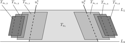
Figure 4. The addition of the six parallelograms $T_{u_{i,1}},T_{u_{i,2}},\ldots,T_{u_{i,6}}$ to the trapezoid $T_{u_{i}}$, ${i=1,2,\ldots,m}$, in the construction of the trapezoid graph $H_{\phi}$ from $G_{\phi}$.

Theorem 3.2.

The formula $\phi$ is NAE-satisfiable if and only if the trapezoid graph $H_{\phi}$ is a bounded tolerance graph.

For the sufficiency part of the proof of Theorem 3.2, the algorithm Split-All plays a crucial role. Namely, given the parallelogram graph $H_{\phi}$ (which is acyclic trapezoid by Lemma 2.3), we construct with this algorithm the acyclic permutation graph $P_{\phi}$ and then a NAE-satisfying assignment of the formula $\phi$. Since monotone-NAE-3-SAT is NP-complete, the problem of recognizing bounded tolerance graphs is NP-hard by Theorem 3.2. Moreover, since this problem lies in NP [15], we summarize our results as follows.

Theorem 3.3.

Given a graph $G$, it is NP-complete to decide whether it is a bounded tolerance graph.

4. The recognition of tolerance graphs

In this section we show that the reduction from the monotone-NAE-3-SAT problem to the problem of recognizing bounded tolerance graphs presented in Section 3, can be extended to the problem of recognizing general tolerance graphs. In particular, we prove that the constructed trapezoid graph $H_{\phi}$ is a tolerance graph if and only if it is a bounded tolerance graph. Then, the main result of this section follows.

Theorem 4.1.

Given a graph $G$, it is NP-complete to decide whether it is a tolerance graph. The problem remains NP-complete even if the given graph $G$ is known to be a trapezoid graph.

5. Concluding remarks

In this article we proved that both tolerance and bounded tolerance graph recognition problems are NP-complete, by providing a reduction from the monotone-NAE-3-SAT problem, thus answering a longstanding open question. The recognition of unit and of proper tolerance graphs, as well as of any other subclass of tolerance graphs, except bounded tolerance and bipartite tolerance graphs [5], remain interesting open problems [14].

References

- [1] S. F. Altschul, W. Gish, W. Miller, E. W. Myers, and D. J. Lipman. Basic local alignment search tool. Journal of molecular biology, 215(3):403–410, 1990.
- [2] K. P. Bogart, P. C. Fishburn, G. Isaak, and L. Langley. Proper and unit tolerance graphs. Discrete Applied Mathematics, 60(1-3):99–117, 1995.
- [3] A. Brandstädt, V. B. Le, and J. P. Spinrad. Graph classes: a survey. SIAM Monographs on Discrete Mathematics and Applications, 1999.
- [4] A. H. Busch. A characterization of triangle-free tolerance graphs. Discrete Applied Mathematics, 154(3):471–477, 2006.
- [5] A. H. Busch and G. Isaak. Recognizing bipartite tolerance graphs in linear time. In Proceedings of the 33rd International Workshop on Graph-Theoretic Concepts in Computer Science (WG), pages 12–20, 2007.
- [6] F. Cheah and D. G. Corneil. On the structure of trapezoid graphs. Discrete Applied Mathematics, 66(2):109–133, 1996.
- [7] F. Cheah and D. G. Corneil, 2009. Personal communication.
- [8] S. Felsner. Tolerance graphs and orders. Journal of Graph Theory, 28:129–140, 1998.
- [9] P. C. Fishburn and W. Trotter. Split semiorders. Discrete Mathematics, 195:111–126, 1999.
- [10] M. C. Golumbic. Algorithmic graph theory and perfect graphs (Annals of Discrete Mathematics, Vol. 57). North-Holland Publishing Co., 2nd edition, 2004.
- [11] M. C. Golumbic and C. L. Monma. A generalization of interval graphs with tolerances. In Proceedings of the 13th Southeastern Conference on Combinatorics, Graph Theory and Computing, Congressus Numerantium 35, pages 321–331, 1982.
- [12] M. C. Golumbic, C. L. Monma, and W. T. Trotter. Tolerance graphs. Discrete Applied Mathematics, 9(2):157–170, 1984.
- [13] M. C. Golumbic and A. Siani. Coloring algorithms for tolerance graphs: reasoning and scheduling with interval constraints. In Proceedings of the Joint International Conferences on Artificial Intelligence, Automated Reasoning, and Symbolic Computation (AISC/Calculemus), pages 196–207, 2002.
- [14] M. C. Golumbic and A. N. Trenk. Tolerance graphs. Cambridge Studies in Advanced Mathematics, 2004.
- [15] R. B. Hayward and R. Shamir. A note on tolerance graph recognition. Discrete Applied Mathematics, 143(1-3):307–311, 2004.
- [16] G. Isaak, K. L. Nyman, and A. N. Trenk. A hierarchy of classes of bounded bitolerance orders. Ars Combinatoria, 69, 2003.
- [17] M. Kaufmann, J. Kratochvíl, K. A. Lehmann, and A. R. Subramanian. Max-tolerance graphs as intersection graphs: cliques, cycles, and recognition. In Proceedings of the 17th annual ACM-SIAM symposium on Discrete Algorithms (SODA), pages 832–841, 2006.
- [18] J. M. Keil and P. Belleville. Dominating the complements of bounded tolerance graphs and the complements of trapezoid graphs. Discrete Applied Mathematics, 140(1-3):73–89, 2004.
- [19] L. Langley. Interval tolerance orders and dimension. PhD thesis, Dartmouth College, 1993.
- [20] T.-H. Ma and J. P. Spinrad. On the 2-chain subgraph cover and related problems. Journal of Algorithms, 17(2):251–268, 1994.
- [21] G. B. Mertzios and D. G. Corneil. Vertex splitting and the recognition of trapezoid graphs. Technical Report AIB-2009-16, Department of Computer Science, RWTH Aachen University, September 2009.
- [22] G. B. Mertzios, I. Sau, and S. Zaks. A new intersection model and improved algorithms for tolerance graphs. SIAM Journal on Discrete Mathematics, 23(4):1800–1813, 2009.
- [23] G. B. Mertzios, I. Sau, and S. Zaks. The recognition of tolerance and bounded tolerance graphs is NP-complete. Technical Report AIB-2009-06, Department of Computer Science, RWTH Aachen University, April 2009.
- [24] G. Narasimhan and R. Manber. Stability and chromatic number of tolerance graphs. Discrete Applied Mathematics, 36:47–56, 1992.
- [25] S. P. Ryan. Trapezoid order classification. Order, 15:341–354, 1998.
- [26] J. P. Spinrad. Efficient graph representations, volume 19 of Fields Institute Monographs. American Mathematical Society, 2003.