A harmonic Lanczos bidiagonalization method for computing interior singular triplets of large matrices

Abstract

This paper proposes a harmonic Lanczos bidiagonalization method for computing some interior singular triplets of large matrices. It is shown that the approximate singular triplets are convergent if a certain Rayleigh quotient matrix is uniformly bounded and the approximate singular values are well separated. Combining with the implicit restarting technique, we develop an implicitly restarted harmonic Lanczos bidiagonalization algorithm and suggest a selection strategy of shifts. Numerical experiments show that one can use this algorithm to compute interior singular triplets efficiently.

1 Introduction

The singular value decomposition (SVD) of a matrix $A\in R^{M\times N},M\geq N$ is given by

$$A=U\Sigma V^{\rm T},$$ (1)

where $\Sigma=diag(\sigma_{1},\sigma_{2},\cdots,\sigma_{N})$, $U=(u_{1},u_{2},\cdots,u_{M})$ and $V=(v_{1},v_{2},\cdots,v_{N})$ are orthogonal matrices of order $M$ and $N$ respectively. $(\sigma_{i},u_{i},v_{i}),i=1,2,\cdots N,$ are called the singular triplets of $A$.

Consider the $(M+N)\times(M+N)$ augmented matrix

$$\tilde{A}=\left(\begin{array}[]{cc}0&A\\ A^{\rm T}&0\end{array}\right).$$ (2)

Then, the eigenvalues of $\tilde{A}$ are $\pm\sigma_{1},\pm\sigma_{2},\cdots,\pm\sigma_{N}$ and $M-N$ zeros. The eigenvectors associated with $\sigma_{i}$ and $-\sigma_{i}$ are $\frac{1}{\sqrt{2}}\left(u_{i}^{\rm T},v_{i}^{\rm T}\right)^{\rm T}$ and $\frac{1}{\sqrt{2}}\left(u_{i}^{\rm T},-v_{i}^{\rm T}\right)^{\rm T}$ respectively. Therefore, the SVD problems are equivalent to the eigenproblems of augmented matrices.

The SVD methods are widely used in determination of numerical rank, determination of spectral condition number, least square problems, regression analysis, image processing, signal processing, pattern recognition, information retrieval, and so on.

At present, computation of largest or smallest singular triplets of large matrices has been well studied, Lanczos bidiagonalization method and its variants are the most popular methods. In 1981, Golub et al. golub1981 firstly designed a block Lanczos bidiagonalization method to compute some largest singular triplets. Larsen larsen1998 discussed the reorthogonalization of the Lanczos bidiagonalization process. Jia and Niu jianiu2003 proposed a refined Lanczos bidiagonalization method to compute some largest and smallest singular triplets. Kokiopoulou et al. kokio2004 used the harmonic projection technique to compute the smallest singular values. Baglama and Reichel baglama2005 ; baglama2006 used Ritz values and harmonic Ritz values to approximate the largest and smallest singular values respectively. Hernandez et al. hernandez2008 provided a parallel implementation of the Lanczos bidiagonalization method. Stoll stoll2008 developed a Krylov-schur approch to partial SVD. Recently, Jia and Niu jianiu2009 proposed a refined harmonic Lanczos bidiagonalization method to compute some smallest singular triplets. All of above methods compute the Lanczos bidiagonalization process, build two $m-$dimensional Krylov subspaces, then extract approximate singular triplets from these two subspace by different ways. Hochstenbach hochstenbach2001 ; hochstenbach2004 also give the Jacobi-Davidson type algorithms for SVD problems.

Due to the storage requirement and the computational cost, all the projection methods must be restarted. The implicit restarting technique sorensen1992 proposed by Sorensen is the most powerful tool and is widely used in many projection methods. The success of this technique heavily depends on the selection of the shifts, see jia1999 ; sorensen1992 . For eigenvalue problems, Sorensen sorensen1992 used the unwanted Ritz values as the shifts to restart Arnoldi method, and Morgan morgan2006 used the unwanted harmonic Ritz values as the shifts to restart harmonic Arnoldi method. Jia jia1999 ; jia2002 used the refined shifts and refined harmonic shifts obtained by the information of the refined Ritz vectors and refined harmonic vectors to restart refined Arnoldi method and refined harmonic Arnoldi method, respectively. For SVD problems, Kokiopoulou et al. kokio2004 used the unwanted harmonic Ritz values as the shifts. Baglama and Reichel baglama2005 ; baglama2006 explicitly augmented the Lanczos bidiagonalization method with certain Ritz vectors or harmonic Ritz vectors. Jia and Niu jianiu2003 ; jianiu2009 gave an refined (harmonic) shift strategy within the implicitly restarted refined (harmonic) Lanczos bidiagonalization method.

In this paper, we are concerned with the computation of interior singular triplets. For a given target $\tau$, we want to compute some singular triplets nearest $\tau$. So, we sort the singular triplets by

$$|\sigma_{1}-\tau|\leq|\sigma_{2}-\tau|\leq\cdots\leq|\sigma_{N}-\tau|.$$ (3)

We must emphasize that, in this paper, $\sigma_{1}$ is the singular value nearest $\tau$ rather than the smallest singular value, meanwhile, $\sigma_{N}$ is the singular value farthest from $\tau$ rather than the largest singular value.

Since the largest eigenvalues of $(\tilde{A}-\tau I)^{-1}$ are the eigenvalues of $\tilde{A}$ closest to $\tau$, and the SVD problem of $A$ is equivalent to the eigenproblem of $\tilde{A}$, we can use shift-invert technique on $\tilde{A}-\tau I$ to compute the interior singular triplets, such as shift-and-invert Arnoldi method (svds). In this paper, we assume that $M$ and $N$ are large and that $A$ can not be factorized. The shift-and-invert technique need the factorization of $\tilde{A}-\tau I$. Since $M$ and $N$ are large, $M+N$, the dimension of $\tilde{A}-\tau I$, is larger. We can not do any factorizations on $\tilde{A}-\tau I$. Therefore, the shift-and-invert technique is not suitable for interior SVD problems.

Another approach for computing interior singular triplets is the harmonic projection method. The harmonic projection method has been widely used to compute interior eigenpairs, see morgan2000 ; morgan2006 , and has been adopted to combine with Lanczos bidiagonalization methods to compute smallest singular triplets baglama2005 ; baglama2006 ; kokio2004 ; jianiu2003 . However, if we use the harmonic projection method explicitly on $\tilde{A}-\tau I$, the scale of the problem is increased and this leads to the increasing computational cost. Further, we ignore the special structure of $\tilde{A}$ or $\tilde{A}-\tau I$, and the projected matrix and the updated process of implicit restarting may lose this structure. Therefore, we must use the harmonic projection method implicitly. Until now, no literature has been appeared to compute interior singular triplets by the harmonic projection method implicitly.

In this paper, we propose a harmonic Lanczos bidiagonalization method for computing interior singular triplets by combining the harmonic projection technique with the Lanczos bidiagonalization process. We analyze the convergence behavior, show that the harmonic Ritz approximations converge to the desired interior singular triplets if some Rayleigh quotient matrix is uniformly bounded and the harmonic Ritz values are well separated. Then, based on Morgan’s harmonic shift strategy morgan2006 for computing interior eigenvalues, we give a selection of the shifts within the framework of the implicitly restarted harmonic Lanczos bidiagonalization methods. Further, we report some numerical experiments of computation of interior singular triplets. It appears that the algorithm we proposed is suitable for computing the interior singular triplets of large matrices.

Throughout this paper, denote by $||\cdot||$ the spectral norm of a matrix and the vector 2-norm, by ${\cal K}_{m}(C,v_{1})=span\{v_{1},Cv_{1},\cdots,C^{m-1}v_{1}\}$ the $m-$ dimensional Krylov subspace generated by the matrix $C$ and the starting vector $v_{1}$, by superscript ’^T’ the transpose of matrix or vector, by $e_{m}$ the $m-$th coordinate vector of dimension $m$.

2 Harmonic Lanczos bidiagonalization method

2.1 Lanczos bidiagonalization process

Golub et al. golub1981 proposed a Lanczos bidiagonalization method to compute the largest singular triplets of $A$. This method is equivalent to the symmetric Lanczos method on $\tilde{A}$ with a special initial vector. It is based on the Lanczos bidiagonalization process, which is shown in matrix form as follows:

$$AQ_{m}=P_{m}B_{m},$$ (4)

$$A^{\rm T}P_{m}=Q_{m}B_{m}^{\rm T}+\beta_{m}q_{m+1}e_{m}^{\rm T},$$ (5)

where

$$B_{m}=\left(\begin{array}[]{c c c c}\alpha_{1}&\beta_{1}&&\\ &\alpha_{2}&\ddots&\\ &&\ddots&\beta_{m-1}\\ &&&\alpha_{m}\end{array}\right)$$ (6)

is an upper bidiagonal matrix, $Q_{m}=(q_{1},q_{2},\ldots,q_{m})$ and $P_{m}=(p_{1},p_{2},\ldots,p_{m})$ span the Krylov subspaces ${\cal K}_{m}(A^{\rm T}A,q_{1})$ and ${\cal K}_{m}(AA^{\rm T},p_{1})$, respectively.

In finite precision arithmetic, the columns of $P_{m}$ and $Q_{m}$ may lose the orthogonality rapidly and must be reorthognalized. From the analysis of Simon and Zha simonzha2000 , we know that only the columns of one of the matrices $P_{m}$ and $Q_{m}$ need to be reorthogonalized. When $M\gg N$, Reorthogonalization on $Q_{m}$ only can reduce the computational cost considerably. So we only perform reorthogonalization on $Q_{m}$.

2.2 Harmonic Lanczos bidiagonalization method

Given the subspace

$${\cal E}=span\left\{\left(\begin{array}[]{cc}P_{m}&0\\ 0&Q_{m}\end{array}\right)\right\}.$$ (7)

Making use of the harmonic projection principle, we compute some approximate eigenpairs $(\theta_{i},\tilde{\varphi}_{i})$ of $\tilde{A}$ nearest $\tau$ by requiring

$$\left\{\begin{array}[]{c}\tilde{\varphi}_{i}\in{\cal E},\\ (\tilde{A}-\theta_{i}I)\tilde{\varphi}_{i}\bot(\tilde{A}-\tau I){\cal E}.\end{array}\right.$$ (8)

From (4) and (5), (8) can be rewritten as the following generalized eigenproblem:

$$\left(\begin{array}[]{cc}-\tau I&B_{m}\\ B_{m}^{\rm T}&-\tau I\end{array}\right)\left(x_{i}\atop y_{i}\right)=\frac{1}{\theta_{i}-\tau}\left(\begin{array}[]{cc}\tau^{2}I+B_{m}B_{m}^{\rm T}+\beta_{m}e_{m}e_{m}^{\rm T}&-2\tau B_{m}\\ -2\tau B_{m}^{\rm T}&\tau^{2}I+B_{m}^{\rm T}B_{m}\end{array}\right)\left(x_{i}\atop y_{i}\right).$$ (9)

Assume that $\theta_{i}>0,i=1,2,\cdots,k+l$, which are sorted by

$$|\theta_{1}-\tau|\leq|\theta_{2}-\tau|\leq\cdots\leq|\theta_{k+l}-\tau|$$

and $\theta_{i}<0,i=k+l+1,k+l+2,\cdots,2m$. We can use $\theta_{i},i=1,2,\cdots,k$ and $\tilde{\varphi}_{i}=\left(P_{m}x_{i}\atop Q_{m}y_{i}\right)$ as the approximation of the desired eigenpair of $\tilde{A}$. Because of the relation between the singular triplets of $A$ and the eigenpairs of $\tilde{A}$, we use $\theta_{i},\tilde{u}_{i}=P_{m}x_{i}/||x_{i}||=P_{m}\tilde{x}_{i},\tilde{v}_{i}=Q_{m}y_{i}/||y_{i}||=Q_{m}\tilde{y}_{i},i=1,2,\cdots,k$ as the approximate singular triplets of $A$ nearest $\tau$. Here we call $\theta_{i},\tilde{u}_{i},\tilde{v}_{i}$ the harmonic Ritz value, the left and right harmonic Ritz vector, respectively.

From (4) and (5), we have

$$||A\tilde{v}_{i}-\theta_{i}\tilde{u}_{i}||=||B_{m}\tilde{y}_{i}-\theta_{i}\tilde{x}_{i}||,$$

$$||A\tilde{v}_{i}-\theta_{i}\tilde{u}_{i}||=\sqrt{||B_{m}^{\rm T}\tilde{x}_{i}-\theta_{i}\tilde{y}_{i}||^{2}+\beta_{m}^{2}|e_{m}^{\rm T}\tilde{x}_{i}|^{2}}.$$

Therefore, if

$$\sqrt{||B_{m}\tilde{y}_{i}-\theta_{i}\tilde{x}_{i}||^{2}+||B_{m}^{\rm T}\tilde{x}_{i}-\theta_{i}\tilde{y}_{i}||^{2}+\beta_{m}^{2}|e_{m}^{\rm T}\tilde{x}_{i}|^{2}}<tol,$$ (10)

where $tol$ is a prescribed tolerance, then the method is known as convergent. So we need not form $\tilde{u}_{i}$ and $\tilde{v}_{i}$ explicitly before convergence.

2.3 Convergence analysis

Set

$$\tilde{B}=\left(\begin{array}[]{cc}-\tau I&B_{m}\\ B_{m}^{\rm T}&-\tau I\end{array}\right)$$

and

$$\tilde{C}=\left(\begin{array}[]{cc}\tau^{2}I+B_{m}B_{m}^{\rm T}+\beta_{m}e_{m}e_{m}^{\rm T}&-2\tau B_{m}\\ -2\tau B_{m}^{\rm T}&\tau^{2}I+B_{m}^{\rm T}B_{m}\end{array}\right),$$

then $\theta_{i},i=1,2,\cdots,2m$ are the eigenvalues of $\tilde{B}^{-1}\tilde{C}$. The matrix $\tilde{B}$ is called the Rayleigh quotient matrix of $\tilde{A}$ with respect to the subspace ${\cal E}$ and the target $\tau$.

The following results are direct from Theorem 2.1, Corollary 2.2 and Theorem 3.2 of jia2005 .

Theorem 2.1

Assume that $(\sigma,u,v)$ is a singular triplet of $A$, define that $\epsilon=\sin\angle\left(\left(u\atop v\right),{\cal E}\right)$ is the distance between the vector $\left(u\atop v\right)$ and the subspace ${\cal E}$. Then there exists a perturbation matrix F such that $\sigma$ is an exact eigenvalue of $\tilde{B}^{-1}\tilde{C}+F$, where

$$||F||\leq\frac{\epsilon}{\sqrt{1-\epsilon^{2}}}||\tilde{B}^{-1}||(\sigma||A||+||A||^{2}).$$ (11)

Furthermore, there exists an eigenvalue of $\tilde{B}^{-1}\tilde{C}$ satisfying

$$|\theta-\sigma|\leq(2||A||+||F||)||F||.$$ (12)

Theorem 2.1 shows that if $\epsilon$ tends to zero and if $||\tilde{B}^{-1}||$ is uniformly bounded, then there exists one harmonic Ritz value $\theta$ converging to the desired singular value $\sigma$.

However, from the interlacing theorem of eigenvalues golub1996 , since

$$\tilde{B}=\left(\begin{array}[]{cc}P_{m}&0\\ 0&Q_{m}\end{array}\right)^{\rm T}(\tilde{A}-\tau I)\left(\begin{array}[]{cc}P_{m}&0\\ 0&Q_{m}\end{array}\right),$$

we have that the eigenvalues of $\tilde{B}$ are between the largest and smallest eigenvalue of $\tilde{A}-\tau I$. Therefore, $\tilde{B}$ may be singular, which leads to arbitrarily large $\|\tilde{B}^{-1}\|$. Hence, we must assume $\|\tilde{B}^{-1}\|$ is uniformly bounded. In fact, this is the inherent defect of the harmonic projection methods, which can be easily obtained from Jia’s analysis jia2005 .

Similarly to the analysis in jia2005 , if $\tau$ is very close to a desired singular value $\sigma$ of $A$, then the method may miss it. We replace $\theta_{i}$ by the Rayleigh-quotient $\rho_{i}=\tilde{u}_{i}^{T}A\tilde{v}_{i}=\tilde{x}_{i}^{T}B_{m}\tilde{y}_{i}$ as the approximate singular value, as was done in hochstenbach2004 ; jianiu2009 . In general, $\rho_{i}$ is more accurate than $\theta_{i}$.

Theorem 2.2

Let $(\theta,z)$ be an eigenpair of $\tilde{B}^{-1}\tilde{C}$, where $z=\left(x\atop y\right)$, and assume $(z,Z_{\bot})$ to be orthogonal such that

$$\left(z^{\rm T}\atop Z_{\bot}^{\rm T}\right)\tilde{B}^{-1}\tilde{C}(z,Z_{\bot})=\left(\begin{array}[]{cc}\theta&g^{\rm T}\\ 0&G\end{array}\right).$$ (13)

If

$$sep(\theta,G)=||(G-\theta I)^{-1}||^{-1}>0,$$ (14)

then

$$\sin\angle\left(\left(u\atop v\right),\left(\tilde{u}\atop\tilde{v}\right)\right) \leq \left(1+\frac{2||\tilde{B}^{-1}||||A||}{\sqrt{1-\epsilon^{2}}sep(\sigma,G)}\right)\varepsilon$$ (15)

$$\leq \left(1+\frac{2||\tilde{B}^{-1}||||A||}{\sqrt{1-\epsilon^{2}}(sep(\theta,G)-|\sigma-\theta|)}\right)\varepsilon.$$

Theorem 2.2 shows that if $\|\tilde{B}^{-1}\|$ is uniformly bounded and $sep(\theta,G)$ is bounded below by a positive constant, that is, all harmonic Ritz values are well separated, then the harmonic Ritz vectors $\tilde{u},\tilde{v}$ converge to the desired left and right singular vector.

3 Implicit restarting technique, shifts selection and an adaptive shifting strategy

3.1 Implicit restarting technique

Due to the storage requirement and the computational cost, the number of Lanczos bidiagonalization steps $m$ can not be large. However, for a relatively small $m$, the approximate singular triplets do not converge. Therefore, the method must be restarted generally.

The implicit restarting technique proposed by Sorensen sorensen1992 is a powerful restarting tool for the Lanczos and Arnoldi process, and has been adopted to the Lanczos bidiagonalization process bjorck1994 ; jianiu2003 ; jianiu2009 ; kokio2004 ; larsen . After running the implicit QR iteration $p$ steps on $B_{m}$ and using the shifts $\mu_{j},j=1,2,\cdots,p$, we have

$$\left\{\begin{array}[]{l}(B_{m}^{\rm T}B_{m}-\mu_{1}^{2}I)\cdots(B_{m}^{\rm T}B_{m}-\mu_{p}^{2}I)=\tilde{P}R,\\ \tilde{P}^{\rm T}B_{m}\tilde{Q}\mbox{ upper bidiagonal},\end{array}\right.$$ (16)

where $\tilde{P},\tilde{Q}$ are the products of the left and right Givens rotation matrices applied to $B_{m}$.

Performing the above process gives the following relation:

$$AQ_{m-p}^{+} = P_{m-p}^{+}B_{m-p}^{+},$$ (17)

$$A^{\rm T}P_{m-p}^{+} = Q_{m-p}^{+}{B_{m-p}^{+}}^{\rm T}+(\beta_{m-p}\tilde{p}_{m,m-p}q_{m+1}+\beta_{m-p}^{+}q_{m-p+1}^{+})e_{m-p}^{\rm T},$$ (18)

where $Q_{m-p}^{+}$ and $q_{m-p+1}^{+}$ are the first $m-p$ columns and the $(m-p+1)$-th column of $Q_{m}\tilde{Q}$, $P_{m-p}^{+}$ is the first $m-p$ columns of $P_{m}\tilde{P}$, $B_{m-p}^{+}$ is the leading $(m-p)\times(m-p)$ block of $\tilde{P}B_{m}\tilde{Q}$, $\tilde{p}_{m,m-p}$ is the $(m,m-p)$ element of $\tilde{P}$. Since $\beta_{m-p}\tilde{p}_{m,m-p}q_{m+1}+\beta_{m-p}^{+}q_{m-p+1}^{+}$ is orthogonal to $Q_{m-p}^{+}$, we obtain a $(m-p)$-step Lanczos bidiagonalization process starting with $q_{1}^{+}$, where

$$\gamma q_{1}^{+}=\prod_{j=1}^{p}(A^{\rm T}A-\mu_{j}^{2}I)q_{1}$$ (19)

with $\gamma$ a factor making $\|q_{1}^{+}\|=1$. It is then extended to the $m$-step Lanczos bidiagonalization process in a standard way.

3.2 shifts selection and adaptive shifting strategy

Once the shifts $\mu_{1},\mu_{2},\ldots,\mu_{p}$ are given, we can run the implicitly restarted algorithm described above iteratively. The success of the implicit restarting technique heavily depends on the selection of the shifts. As is shown in jianiu2003 , from (19), it can be easily seen that the more accurate the shifts approximate to some unwanted singular values, the more information on the unwanted singular vectors are dampened out after restarting. Therefore, the resulting subspace contains more information on the desired singular vectors, and the algorithms may converge faster. For eigenproblems and SVD problems, Morgan morgan2006 and Kokiopoulou et al. kokio2004 suggested using the unwanted harmonic Ritz values as shifts. A natural choice of the shifts within our algorithm is the unwanted approximate singular values $\theta_{k+j},j=1,2,\cdots,l$, since they are the best approximations available to some of the unwanted singular values within our framework.

From (19), we see the component along the desired $k$-th singular vector $u_{k}$ is greatly damped if a shift $\mu_{i}$ is very close to $\sigma_{k}$, so $\mu_{i}$ is a bad shift and $\rho_{k}$ may converge to $\sigma_{k}$ very slowly or not at all. To correct this problem, Larsen larsen proposed an adaptive strategy to compute largest singular triplets. He replaces a bad shift by zero shift. Jia and Niu jianiu2003 ; jianiu2009 gave a modified form for computing smallest singular triplets. Define the relative gaps of $\rho_{k}$ and all the shifts $\mu_{i},i=1,2,\cdots,l$ by

$${\rm relgap}_{ki}=\left|\frac{(\rho_{k}-\varepsilon_{k})-\mu_{i}}{\rho_{k}}\right|,$$ (20)

where $\varepsilon_{k}$ is the residual norm (10). If ${\rm relgap}_{ki}\leq 10^{-3}$, $\mu_{i}$ is a bad shift and should be replaced by a suitable quantity. They replace the bad shifts by the largest or the smallest approximate singular value for computing the smallest or the largest singular triplets. In this paper, a good strategy is replacing the bad shifts by the approximate singular value farthest from $\tau$, as this strategy amplifies the components of $q_{1}^{+}$ in $v_{i},i=1,2,\cdots,k$ and damps those in $v_{i},i=k+1,k+2,\cdots,N$.

4 Numerical Experiments

Numerical experiments are carried out using Matlab 7.1 R14 on an Intel Core 2 E6320 with CPU 1.86GHZ and 2GB of memory under the Window XP operating system. Machine epsilon is $\epsilon_{\rm mach}\approx 2.22\times 10^{-16}$. The stopping criteria is

$$stopcrit=\max_{1\leq i\leq k}\sqrt{\|A\tilde{v}_{i}-\rho_{i}\tilde{u}_{i}\|^{2}+\|A^{\rm T}\tilde{u}_{i}-\rho_{i}\tilde{v}_{i}\|^{2}}.$$ (21)

If

$$\frac{stopcrit}{\|A\|_{1}}<tol,$$ (22)

then stop. From (10), we need not form $\tilde{u}_{i},\tilde{v}_{i}$ explicitly before convergence.

For large eigenproblems, in order to speed up convergence, most of the implicitly restarted Krylov type subspace algorithms, such as ARPACK(eigs), compute $k+3$ approximate eigenpairs when $k$ eigenpairs are desired. This strategy has been adopted to SVD problems, see baglama2005 ; jianiu2009 . In this paper, we also compute $k+3$ approximate singular triplets and use $l-3$ shifts in implicit restarting process.

All test matrices are from bai1997 . We take $tol=10^{-6}$. In all the tables, ’$iter$’ denotes the number of restart, ’$time$’ denotes the CPU timings in second, ’$mv$’ denotes the number of matrix-vector products. Since the matrix-vector products performed on $A$ are equal to those on $A^{\rm T}$, we only count the matrix-vector products on $A$.

4.1 Computation of smallest singular triplets

Obviously, we can compute some smallest singular triplets by taking $\tau=0$. We compute three singular triplets nearest $\tau=0,0.01,0.005,0.001$ of WELL1850, respectively. These three singular values are all the three smallest singular values. The computed three singular values are

$$\sigma_{1}\approx 1.611969e-002,\sigma_{2}\approx 1.911309e-002,\sigma_{3}\approx 2.315889e-002.$$

Table 1 reports the computational results. Fig. 1 plots the absolute residual norms of the computed singular triplets for $m=15$ and $m=20$, respectively. From Table 1 and Fig. 1, we see that for all $\tau$, our algorithm can compute three singular triplets accurately. However, for different $\tau$, the algorithm has a great difference on restart numbers, matrix-vector products and CPU times. This phenomenon shows a good choice of target point $\tau$ can speed up the convergence considerably.

Table 1: WELL1850 for $k=3$, $m=10,15,20,25$, $\tau=0,0.001,0.005,0.01$

$m$	$iter$	$time$	$mv$	$stopcrit$	$iter$	$time$	$mv$	$stopcrit$
	$\tau=0$				$\tau=0.001$
10	543	5.15	2178	1.67e-005	178	1.89	718	1.66e-005
15	119	3.20	1077	1.67e-005	74	1.99	672	1.25e-005
20	56	3.48	790	1.50e-005	48	2.81	678	1.62e-005
25	35	3.20	671	1.35e-005	35	3.64	671	1.14e-005
	$\tau=0.005$				$\tau=0.01$
10	160	1.66	646	1.66e-005	179	1.76	722	1.60e-005
15	68	1.86	618	1.62e-005	64	1.73	582	1.52e-005
20	39	2.31	552	1.08e-005	37	2.23	524	1.45e-005
25	31	3.10	595	1.27e-005	29	2.89	557	1.06e-005

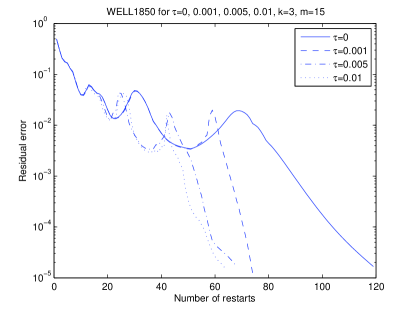
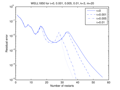
Figure 1: Absolute residual norms for WELL1850 for $k=3$, $m=20$, $\tau=0,0.01,0.005,0.001$

4.2 Computation of three interior singular triplets nearest different $\tau$

The test matrix is DW2048, a $2048\times 2048$ matrix. We compute three singular triplets nearest different $\tau$. The computational results are shown in Tables 2-3. From Table 2, we see that the relative errors of the computed singular values are no more than $O(10^{-9})$. The Tables demonstrate that our algorithm can compute the desired singular triplets accurately.

Table 2: Three computed singular values of DW2048 nearest $\tau=0.2,0.5,0.6,0.8$ for $m=50$

$\tau=0.2$		$\tau=0.5$
$\rho_{j}$	$|\rho_{j}-\sigma_{j}|/\sigma_{j}$	$\rho_{j}$	$|\rho_{j}-\sigma_{j}|/\sigma_{j}$
2.0031301e-001	1.55e-014	4.9933773e-001	1.62e-14
1.9939880e-001	5.90e-014	5.0082218e-001	1.04e-12
1.9813769e-001	1.08e-009	4.9764898e-001	8.76e-11
$\tau=0.6$		$\tau=0.8$
$\rho_{j}$	$|\rho_{j}-\sigma_{j}|/\sigma_{j}$	$\rho_{j}$	$|\rho_{j}-\sigma_{j}|/\sigma_{j}$
6.0106012e-001	4.29e-12	8.0014466e-001	2.41e-12
6.0193472e-001	4.22e-11	7.9954438e-001	5.46e-12
5.9689466e-001	2.40e-13	7.9932106e-001	1.08e-10

Table 3: DW2048 for $k=3$, $m=30,40,50$, $\tau=0.2,0.5,0.6,0.8$

	$\tau=0.2$				$\tau=0.5$
$m$	$iter$	$time$	$mv$	$stopcrit$	$iter$	$time$	$mv$	$stopcrit$
30	501	109	11655	9.97e-007	255	51.2	6123	9.93e-007
40	298	113	9993	9.81e-007	97	38.2	3271	9.90e-007
50	221	136	9652	9.85e-007	83	50.9	3656	9.10e-007
	$\tau=0.6$				$\tau=0.8$
$m$	$iter$	$time$	$mv$	$stopcrit$	$iter$	$time$	$mv$	$stopcrit$
30	125	24.6	3006	9.11e-007	405	78.2	9525	9.87e-007
40	69	27.0	2343	9.47e-007	180	70.4	6079	9.64e-007
50	46	28.1	2012	8.61e-007	136	81.8	5989	9.50e-007

4.3 Computation of interior singular triplets for different $k$

We compute $k=1,3,5,10$ smallest singular triplets nearest $\tau=4.5$ of LSHP2233, a $2233\times 2233$ matrix. Table 5 reports the results. We see that our algorithm can compute the desired singular triplets with high precision.

Table 4: Ten computed singular values of LSHP2233 nearest $\tau=4.5$ for $m=50$

$\rho_{1}$	$|\rho_{1}-\sigma_{1}|/\sigma_{1}$	$\rho_{2}$	$|\rho_{2}-\sigma_{2}|/\sigma_{2}$
4.4988631	1.58e-15	4.5091282	1.36e-14
$\rho_{3}$	$|\rho_{3}-\sigma_{3}|/\sigma_{3}$	$\rho_{4}$	$|\rho_{4}-\sigma_{4}|/\sigma_{4}$
4.5113859	1.22e-14	4.4815289	6.54e-15
$\rho_{5}$	$|\rho_{5}-\sigma_{5}|/\sigma_{5}$	$\rho_{6}$	$|\rho_{6}-\sigma_{6}|/\sigma_{6}$
4.5188882	5.11e-15	4.5210494	1.18e-14
$\rho_{7}$	$|\rho_{7}-\sigma_{7}|/\sigma_{7}$	$\rho_{8}$	$|\rho_{8}-\sigma_{8}|/\sigma_{8}$
4.4783693	1.07e-14	4.4716358	8.74e-15
$\rho_{9}$	$|\rho_{9}-\sigma_{9}|/\sigma_{9}$	$\rho_{10}$	$|\rho_{10}-\sigma_{10}|/\sigma_{10}$
4.5331457	5.68e-15	4.4638926	2.03e-10

Table 5: LSHP2233 for $k=1,3,5,10$, $m=30,40,50$, $\tau=4.5$

	$k=1$				$k=3$
$m$	$iter$	$time$	$mv$	$stopcrit$	$iter$	$time$	$mv$	$stopcrit$
30	467	108	11920	6.88e-006	560	127	13171	6.95e-006
40	190	83.6	6844	6.86e-006	230	98.1	7826	6.79e-006
50	159	114	7188	6.63e-006	216	140	9404	6.66e-006
	$k=5$				$k=10$
$m$	$iter$	$time$	$mv$	$stopcrit$	$iter$	$time$	$mv$	$stopcrit$
30	322	64.8	6972	6.99e-006	651	103	10761	6.91e-006
40	207	78.5	6632	6.78e-006	168	61.0	4548	4.70e-006
50	132	83.8	5487	6.40e-006	165	92.4	6003	6.99e-006

5 Conclusion

In this paper, combining the harmonic projection principle with the implicit restarting technique, we propose an implicitly restarted harmonic Lanczos bidiagonalization algorithm for computing some interior singular triplets. Based on Morgan’s harmonic shift strategy for computing interior eigenpairs, we give a selection of the shifts within our algorithm. Numerical experiments show that our algorithm is suitable for interior SVD problems. The interior singular values can be computed with higher relative precision.

The Matlab code can be obtained from the authors upon request.

- (1) Z. Bai, R. Barret, D. Day, J.Demmel and J.Dongarra, Test matrix collection for non-Hermitian eigenvalue problems, Technical Report CS-97-355, University of Tennessee, Knoxville (1997). Data available at http://math.nist.gov/MarketMatrix.
- (2) J. Baglama and L. Reichel, Augmented implicitly restarted Lanczos bidiagonalization methods, SIAM J. Sci. Comput. 27, 19-42 (2005)
- (3) J. Baglama and L. Reichel, Restarted block Lanczos bidiagonalization methods, Numer. Algor., 43, 251-272 (2006)
- (4) Å. Björck, E. Grimme and P. van Dooren, An implicitly bidiagonalization algorithm for ill-posed systems, BIT, 34 , 510-534 (1994)
- (5) G. H. Golub, F. T. Luk and M. L. Overton, A block Lanczos method for computing the singular values and singular vectors of a matrix, ACM Trans. Math. Soft., 7, 149-169 (1981)
- (6) G. H. Golub and C. F. Van Loan, Matrix Computations, 3rd ed., page 396, The Johns Hopkins University Press, Baltimore (1996)
- (7) V Hernandez, J. E. Roman, A. Tomas, V. Vidal, A robust and efficient parallel SVD solver based on restarted Lanczos bidiagonalization, ETNA, 31, 68-85 (2008)
- (8) M. E. Hochstenbach, A Jacobi-Davidson type SVD method, SIAM J. Sci. Comput., 23, 606 (2001)
- (9) M. E. Hochstenbach, Harmonic and refined extraction methods for the singular value prob- lem, with applications in least squares problems, BIT, 44, 721-754 (2004)
- (10) Z. Jia, Polynomial characterizations of the approximate eigenvectors by the refined Arnoldi method and an implicitly restarted refined Arnoldi algorithm, Linear Algebra Appl., 287 , 191-214 (1999)
- (11) Z. Jia, The refined harmonic Arnoldi method and an implicitly restarted refined algorithm for computing interior eigenpairs of large matrices, Appl. Numer. Appl., 42 , 489-512 (2002)
- (12) Z. Jia, The convergence of harmonic Ritz values, harmonic Ritz vectors and re ned harmonic Ritz vectors, Math. Comput., 74, 1441-1456 (2005)
- (13) Z. Jia and D. Niu, An implicitly restarted refined bidiagonalization Lanczos method for computing a partial singular value decomposition, SIAM J. Matrix Anal. Appl., 25, 246-265 (2003)
- (14) Z. Jia and D. Niu, A refined harmonic Lanczos bidiagonalization method and an implicitly restarted algorithm for computing the smallest singular triplets of large matrices, Siam J. Sci. Comp., to appear.
- (15) E. Kokiopoulou, C. Bekas and E. Gallopoulos, Computing smallest singular triplets with implicitly restarted Lanczos bidiagonalization, Appl. Numer. Math., 49, 39-61 (2004)
- (16) R. M. Larsen, Lanczos bidiagonalization with partial reorthogonalization, Chapter of Ph.D. thesis, Department of Computer Science, University of Aarhus, Danmark (1998)
- (17) R. M. Larsen, Combining implicit restarts and partial reorthogonalization in Lanczos bidiagonalization, http://soi.stanford.edu/ rmunk/PROPACK.
- (18) R. B. Morgan and M. Zeng, Implicitly restarted GMRES and Arnoldi methods for nonsymmetric linear systems of equations, SIAM J. Matrix Anal. Appl., 21, 1112-1135 (2000)
- (19) R. B. Morgan, A harmonic restarted Arnoldi algorithm for calculating eigenvalues and determining multiplicity, Linear Algebra Appl., 415, 96-113 (2006)
- (20) H. D. Simon and H. Zha, Low-rank matrix approximation using the Lanczos bidiagonalization process with applications, SIAM J. Sci. Comput., 21 , 2257 C2274 (2000).
- (21) D. C. Sorensen, Implicit application of polynomial filters in a k-step Arnoldi method, SIAM J. Matrix Anal. Appl., 13, 357-385 (1992)
- (22) M. Stoll, A Krylov-Schur approach to the truncated SVD, NA-08-03, Laboratory of Computing Laboratory, Oxford University (2008)