Glassy Freezing and Long-Range Order in the $3D$ Random Field $XY$ Model

Abstract

Monte Carlo studies of the 3D random field $XY$ model on simple cubic lattices of size $64^{3}$, using two different isotropic random-field probability distributions of moderate strength, show a glassy freezing behavior above $T_{c}$, and long-range order below $T_{c}$, consistent with our earlier results for weaker and stronger random fields. This model should describe random pinning in vortex lattices in type-II superconducting alloys, charge-density wave materials, and decagonal quasicrystals.

The random-field XY model (RFXYM) was first studied forty years ago,Lar70 as a toy model for random pinning effects in the vortex lattice of a type-II superconductor in an external magnetic field. For fixed-length classical spins the Hamiltonian of the RFXYM is

$$H~{}=~{}-J\sum_{\langle ij\rangle}\cos(\phi_{i}-\phi_{j})~{}-~{}\sum_{i}h_{i}\cos(\phi_{i}-\theta_{i})\,.$$ (1)

Each $\phi_{i}$ is a dynamical variable which takes on values between 0 and $2\pi$. The $\langle ij\rangle$ indicates here a sum over nearest neighbors on a simple cubic lattice of size $L\times L\times L$. We choose each $\theta_{i}$ to be an independent identically distributed quenched random variable, with the flat probability distribution

$$P(\theta_{i})~{}=~{}1/2\pi\,$$ (2)

for $\theta_{i}$ between 0 and $2\pi$. The probability distribution $P(h_{i})$ is independent of $\theta_{i}$. This Hamiltonian is closely related to models of incommensurate charge density waves,GH96 ; Fis97 which include decagonal and other axial quasicrystalsSJSTAT98 as special cases. In all of these cases, the physical origin of the “random field” is the fact that any real sample contains a finite density of point defects, i.e. atoms sitting in places where they would not be in the ideal structure.

We will use the term “sample” to denote a Hamiltonian with a particular set of the $h_{i}$ and $\theta_{i}$ variables. A thermal average of some quantity over a single sample will be denoted here by angle brackets, $\langle~{}\rangle$, and an average over all samples will be denoted by square brackets, $[~{}]$.

LarkinLar70 replaced the spin-exchange term of the Hamiltonian with a harmonic potential, so that each $\phi_{i}$ is no longer restricted to lie in a compact interval. This approximation, which neglects mode coupling, is strictly valid only in the limit $n\to\infty$, where $n$ is the number of components for each spin. Larkin then argued that, for any probability distribution $P(h_{i})$ which allows non-zero values for $h_{i}$, this model has no long-range ordered phase on a lattice whose spatial dimension $d$ is less than or equal to four.

A more intuitive derivation of this result was given by Imry and Ma,IM75 who assumed that the increase in the energy of an $L^{d}$ lattice when the order parameter is twisted at a boundary scales as $L^{d-2}$. This was later justifiedAIM76 ; PS82 by showing that within a perturbative $\epsilon$ expansion one finds the phenomenon of “dimensional reduction”. Term by term for $T>T_{c}$, the critical exponents of any $d$-dimensional $O(n)$ random-field model appear to be identical to those of an ordinary $O(n)$ model of dimension $d-2$.

However, reservations about the correctness of applying the $n=\infty$ results for finite $n$, i.e. the substitution of the harmonic potential for the exchange term, were soon expressed by Grinstein.Grin76 For the Ising ($n=1$) case, dimensional reduction was shown rigorously to be incorrect.Imb84 ; BK87

One problem with dimensional reduction for $n>1$ is that the perturbation theory can only be calculated for $T>T_{c}$, while the twist energy of the order parameter is only defined for $T<T_{c}$. Another, more interesting problem for $n>1$ is associated with the question of properly defining the order parameter. As discussed, for example, by Griffiths,Grif66 there is more than one way to do this. For the random-field model, there are several different types of two-point correlation functions.Grin76

When $n=2$, one may use the vector order parameter $\vec{\bf M}$, defined by

$$\vec{\bf M}~{}=~{}N^{-1}\sum_{i}\cos(\phi_{i})\hat{x}~{}+~{}\sin(\phi_{i})\hat{y}\,,$$ (3)

where $N=L^{d}$ is the number of spins. Alternatively, one can choose the scalar order parameter $M^{2}$, defined by

$$M^{2}~{}=~{}N^{-2}\sum_{i,j}\cos(\phi_{i})\cos(\phi_{j})~{}+~{}\sin(\phi_{i})\sin(\phi_{j})\,.$$ (4)

It is very awkward to calculate $\vec{\bf M}$, since its value will vary wildly from sample to sample. Thus we expect that $[\vec{\bf M}]$ will be zero, even though $\langle\vec{\bf M}\rangle$ for each sample may become large at low temperature. On the other hand, we anticipate that for weak disorder the probability distribution for $M^{2}$ will become narrow as we take $L\to\infty$. Thus it is the quantity $\langle M^{2}\rangle$, and not the quantity $\langle\vec{\bf M}\rangle$, which is the natural carrier of long-range order in the presence of the random field.

It is also necessary to consider the possibility that the thermal average $\langle M^{2}\rangle$ for a typical finite sample may become large as $T$ is lowered, even though $\langle\vec{\bf M}\rangle$ remains small. This will occur when the energy required for reorienting $\langle\vec{\bf M}\rangle$ is nonzero, but not large compared to $T$. If this were to occur, then there would be no local order parameter, and thus no terms in the Landau-Ginsburg free-energy functional which depended on gradients of $\langle\vec{\bf M}\rangle$.

Monte Carlo calculations for Eqn. (1) on simple cubic lattices were performed some time ago by Gingras and HuseGH96 and FischFis97 . More recently, additional calculations were carried out.Fis07 The results of these studies, which used several different choices for the probability distribution $P(h_{i})$, indicate that for typical samples the order parameter $\langle M^{2}\rangle$ becomes positive at some positive temperature $T_{c}$, as long as the random fields are not too strong. However, the precise nature of what happens near $T_{c}$ remained unclear. In this work we report additional studies using new choices of $P(h_{i})$, which display phenomena which were not seen clearly in the earlier studies.

The computer program which was used was an enhanced version of the one used before.Fis07 The data were obtained from $L\times L\times L$ simple cubic lattices with $L=64$ using periodic boundary conditions. Some preliminary studies for smaller values of $L$ were also done. The program approximates $O(2)$ with $Z_{12}$, a 12-state clock model. It was modified to enable the study of random-field probability distributions of the form

$$P(h_{i})~{}=~{}(1-p)\delta(h_{i}-h_{r})~{}+~{}p\delta(h_{i})\,.$$ (5)

This modification makes the program run a few percent slower than before. In this work we study two cases. Type A samples have $h_{r}=1.5$ with $p=0$, and Type B samples have $h_{r}=2$ with $p=0.5$. For both of these cases we find $T_{c}/J$ near 1.5, which was suggested by Gingras and HuseGH96 to be optimal for this sort of calculation.

On a simple cubic lattice of size $L\times L\times L$, the magnetic structure factor, $S(\vec{\bf k})$, for $n=2$ spins is

$$S(\vec{\bf k})~{}=~{}L^{-3}\sum_{i,j}\cos(\vec{\bf k}\cdot\vec{\bf r}_{ij})\langle\cos(\phi_{i}-\phi_{j})\rangle\,,$$ (6)

where $\vec{\bf r}_{ij}$ is the vector on the lattice which starts at site $i$ and ends at site $j$. Thus, setting $\vec{\bf k}$ to zero yields

$$S(0)/L^{3}~{}=~{}\langle M^{2}(L)\rangle\,.$$ (7)

As we will see, the extrapolation of $\langle M^{2}(L)\rangle$ to $L=\infty$ is not trivial.

In this work, we present results for the average over angles of $S(\vec{\bf k})$, which we write as $S(k)$. Eight different $L=64$ samples of the random fields $\theta_{i}$ were used for each $P(h_{i})$. The same samples of random fields were used for all values of $T$.

The Monte Carlo calculations were performed using both hot start (i.e. random) initial conditions followed by slow cooling, and also cold start (i.e. ferromagnetic) initial conditions followed by slow warming. For the Type A samples three different cold start initial conditions were used, equally spaced around the circle. For the Type B samples, where the average random field is somewhat weaker, only two cold start initial conditions were used.

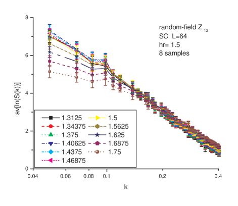
Figure 1: (color online) Average over 8 samples of $\ln(S(k))$ for $64\times 64\times 64$ lattices with $h_{r}=1.5$ and $p=0$ at various temperatures. The error bars indicate approximately three standard deviation statistical errors, and the $x$-axis is scaled logarithmically.

In Fig. 1 we show data for the average over our eight Type A samples of $\ln(S(k))$ for $T/J$ between 1.3125 and 1.75. The data for $T/J\geq 1.4375$ are taken from the hot start runs, and the data for lower values of $T/J$ are taken from the cold start run which gave the lowest average value for the energy, $\langle E\rangle$. When $T=1.4375$ or more, all runs for a given sample converge in a rather short time to give similar values of $\langle E\rangle$ and $\langle\vec{\bf M}\rangle$. However, for lower values of $T/J$ the hot start runs remain stuck in metastable states.

An attempt was made to drive the hot start runs into equilibrium by deep undercooling, followed by slow warming. This thermal cycling technique had proven successful earlier,Fis07 for the weak random field case of $h_{r}=1.0$ with $p=0$. For the cases studied here, however, a single undercooling was only partially successful in driving the samples to equilibrium. The author believes that repeating cycling would have worked successfully. However, since a detailed study of the nonequilibrium behavior was not the purpose of the work described here, this was not attempted.

Somewhat surprisingly, the cold start runs were much more successful in finding a single free energy minimum at $T/J$ between 1.3125 and 1.40625. In the majority of samples, all of the cold start initial conditions were converging to the same free energy minimum. This was no longer true for $T/J<1.3125$, and thus results for these lower temperatures are not reported.

For each sample at each value of $T/J$, the data shown in the figure were obtained by averaging $S(k)$ over 16 spin states taken at intervals of 51,200 Monte Carlo steps per spin (MCS), after letting the sample equilibrate. Thus the length of each data-gathering run was 768,000 MCS. The values shown for $S(k)$ are obtained by averaging over all of the values of $\vec{\bf k}$ which have length $k$. This multiplicity, which is not the same for all values of $k$, was not taken into account in calculating the error bars shown in the figures. Thus each error bar shown in the figures represents approximately three standard deviations. The procedure used for the Type B samples was essentially identical.

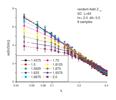
Figure 2: (color online) Average over 8 samples of $\ln(S(k))$ for $64\times 64\times 64$ lattices with $h_{r}=2$ and $p=0.5$ at various temperatures. The error bars indicate approximately three standard deviation statistical errors, and the $x$-axis is scaled logarithmically.

In Fig. 2 we show the corresponding data for the Type B samples, for $T/J$ between 1.4375 and 2.00. The data for $T/J>1.5625$ are taken from the hot start runs, and the data for lower values of $T/J$ are taken from the cold start run which gave the lower average value for the energy, $\langle E\rangle$. It was also true for these Type B samples that the hot start samples were unable to equilibrate on accessible time scales for $T/J\leq 1.5625$.

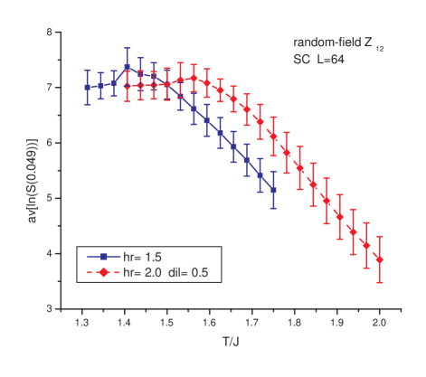
Figure 3: (color online) Average over 8 samples of $\ln(S(\pi/64))$ for $64\times 64\times 64$ lattices as a function of $T/J$. The error bars indicate approximately three standard deviation statistical errors.

We can define $T_{c}$ in a number of ways. For instance, it can be defined as the highest temperature for which we have been unable to equilibrate the hot start runs. It is also the temperature for which the equilibration time for the cold start runs becomes very long. The fact that equilibration times get very long at the same $T_{c}$ for both the hot start and the cold start initial conditions that the behavior of this model can not be explained by the usual hysteresis which is associated with a normal first-order phase transition. As was discussed in somewhat more detail in the earlier work,Fis07 the author believes that this phase transition should be described by a theory of the Anderson-YuvalAY71 type, where the order parameter jumps to zero discontinuously at $T_{c}$. A phase transition of this type is also believed to occur in the k-core percolation model,SLC06 which has been suggested as model for the ordinary glass transition.

The qualitative behavior which we see in Fig. 1 and Fig. 2 is that the average over samples of $\ln(S(k))$ shows a peak at small $k$ which grows in size as we lower $T$, until it reaches a maximum at $T_{c}$. The value of $T_{c}/J$ is about 1.40625 for the Type A samples and 1.5625 for the Type B samples. Upon lowering $T$ below $T_{c}$, the size of the peak becomes somewhat smaller. This is seen more clearly in Fig. 3, which shows the temperature dependence of av[$\ln(S(\pi/64))$] for both types of samples. (The value of $\pi/64$ is approximately 0.049.)

For $T>T_{c}$ both types display a substantial range of $T$ over which $S(\pi/64)$ is increasing exponentially as $T$ is lowered, and this increase slows very close to $T_{c}$. This kind of temperature dependence is well known phenomenologicallyWLF55 to be a characteristic of glassy freezing behavior. However, the reader should keep in mind that one expects the usual glass transition to correspond to $n=3$ spins, and not the $n=2$ spins studied here. If one generalizes Eqn. (1) to the $n=3$ case, substantially more computing resources would be required to make the equivalent calculation feasible.

Below $T_{c}$, $S(\pi/64)$ first decreases, and then becomes approximately constant, at least over the range of $T$ shown in the figure, where the samples are believed to be equilibrated. This behavior below $T_{c}$ is consistent with the existence of a $\delta$-function peak in $S$ at $k=0$ in the limit $L\to\infty$, indicative of true long-range order. One would not expect to see this behavior if there were only power-law correlations in $S(k)$, with no $\delta$-function peak.

The reader should understand that we are not claiming the existence of some mathematical error in the analysisFish97 of the elastic glass, which leads to the power-law correlated Bragg glass phase. That analysis begins with the Larkin Hamiltonian,Lar70 which approximates the spin-exchange term of Eqn. (1) with a harmonic interaction. What we are saying is that the long-range behavior of the Larkin Hamiltonian is different from that of Eqn. (1), at least for the types of $P(h_{i})$ distributions we have studied.

If we fit the data for av[$\ln(S(k))$] at $T_{c}$ over the range $\pi/64\leq k\leq\pi/8$, as shown in Fig. 1 and Fig. 2, we find good straight line fits, with slopes of -3.20(3) for the Type A samples and -3.10(2) for the Type B samples. Because both of these slopes are more negative than -3, it is clearly not correct to extrapolate these fits to $k=0$. $S(k)$ satisfies a sum rule, and thus nonintegrable singularities cannot occur. Thus if we were able to obtain data using these $P(h_{i})$ distributions for even larger values of $L$, we would expect to find that the behavior of av[$\ln(S(k))$] at $T_{c}$ for small enough nonzero $k$ would look like the data for the case $h_{r}=2$ with $p=0$ found in the earlier work.Fis07

In this work we have performed Monte Carlo studies of the 3D RFXYM on $L=64$ simple cubic lattices, with isotropic random field distributions of two types: $h_{r}$ = 1.5 with $p$ = 0, and $h_{r}$ = 2 with $p$ = 0.5. We present results for the structure factor, $S(k)$, at a sequence of temperatures. In agreement with prior resultsFis07 on weaker and stronger random fields, we argue that our results indicate a phase transition into a long-range ordered low temperature phase, with a jump in the order parameter at $T_{c}$. The behavior above $T_{c}$ strongly resembles well known phenomenology for glassy phase transitions.WLF55

- (1) A. I. Larkin, Zh. Eksp. Teor. Fiz. 58, 1466 (1970) [Sov. Phys. JETP 31, 784 (1970)].
- (2) M. J. P. Gingras and D. A. Huse, Phys. Rev. B 53, 15193 (1996).
- (3) R. Fisch, Phys. Rev. B 55, 8211 (1997).
- (4) P. J. Steinhart et al., Nature 396, 55 (1998).
- (5) Y. Imry and S.-K. Ma, Phys. Rev. Lett. 35, 1399 (1975).
- (6) G. Grinstein, Phys. Rev. Lett. 37, 944 (1976).
- (7) A. Aharony, Y. Imry and S.-K. Ma, Phys. Rev. Lett. 36, 1364 (1976).
- (8) G. Parisi and N. Sourlas, Nucl. Phys. B206, 321 (1982).
- (9) J. Z. Imbrie, Phys. Rev. Lett. 53, 1747 (1984).
- (10) J. Bricmont and A. Kupiainen, Phys. Rev. Lett. 59, 1829 (1987).
- (11) R. B. Griffiths, Phys. Rev. 152, 240 (1966).
- (12) R. Fisch, Phys. Rev. B 76, 214435 (2007).
- (13) P. W. Anderson and G. Yuval, J. Phys. C 4, 607 (1971).
- (14) J. M. Schwarz, A. J. Liu and L. Q. Chayes, Europhys. Lett. 73, 560 (2006).
- (15) M. L. Williams, R. F. Landel and J. D. Ferry, J. Am. Chem. Soc. 77, 3701 (1955).
- (16) D. S. Fisher, Phys. Rev. Lett. 78, 1964 (1997).