Comparison of an approximately isothermal gravitational potentials of elliptical galaxies based on X-ray and optical data.

Abstract

We analyze six X-ray bright elliptical galaxies, observed with Chandra and XMM-Newton, and approximate their gravitational potentials by isothermal spheres $\varphi=v_{c}^{2}\log r$ over a range of radii from $\sim$0.5 to $\sim 25$ kpc. We then compare the circular speed $v_{c}$ derived from X-ray data with the estimators available from optical data. In particular we discuss two simple and robust procedures for evaluating the circular speed of the galaxy using the observed optical surface brightness and the line-of-sight velocity dispersion profiles. The best fitting relation between the circular speeds derived from optical observations of stars and X-ray observations of hot gas is $v_{c,opt}\simeq\eta~{}v_{c,X}$, where $\eta=1.10-1.15$ (depending on the method), suggesting, albeit with large statistical and systematic uncertainties, that non-thermal pressure on average contributes $\sim$20-30% of the gas thermal pressure.

1 Introduction

In spiral galaxies, disk rotation curves offer an accurate and robust way of measuring total gravitational potentials to distances as large as 10–30 kpc. To a first approximation the rotation curves are flat over a broad range of radii, suggesting an isothermal (logarithmic) potential characterized by $\varphi(r)=v_{c}^{2}\log r$. In early-type galaxies, measuring the gravitational potential is much more difficult since there are no tracers such as cold gas or disk stars on orbits of known shape. Several methods have been used to measure the potentials of elliptical galaxies including detailed modeling of stellar orbits (Kronawitter et al., 2000; Cappellari et al., 2006; Thomas et al., 2007; Gültekin et al., 2009), tracers such as globular clusters, planetary nebulae, and satellite galaxies (Romanowsky & Kochanek, 2001; Coccato et al., 2009; Klypin & Prada, 2009), strong and weak lensing of quasars and background galaxies (Koopmans et al., 2006; Mandelbaum et al., 2006; Gavazzi et al., 2007; Mandelbaum, van de Ven, & Keeton, 2008) and (for the most massive galaxies) modeling the hydrostatic atmospheres of X-ray emitting gas (Mathews, 1978; Forman, Jones, & Tucker, 1985; Fukazawa et al., 2006; Humphrey et al., 2006; Churazov et al., 2008). Recent studies using stellar kinematics and lensing suggest that the potentials of early-type galaxies are approximately isothermal (Gerhard et al., 2001; Treu et al., 2006; Gavazzi et al., 2007), similar to disk galaxies. Consistency of the mass profile with $M(r)\propto r$ (implying an isothermal potential) was also suggested for several elliptical galaxies based on the analysis of X-Ray data (e.g., Trinchieri & Fabbiano, 1985; Buote & Canizares, 1994; Kim & Fabbiano, 1995; Nulsen & Bohringer, 1995; Buote & Canizares, 1998; Fukazawa et al., 2006). Here we present independent evidence that the potentials of bright elliptical galaxies are close to isothermal, from X-ray observations with Chandra and XMM-Newton. If the potential of a typical elliptical galaxy is indeed not far from being isothermal (for a range of radii) then it can be characterized in that radius range with a single number – the circular speed $v_{c}$. This makes the comparison of potentials derived from X-ray and optical data especially simple since it does not require a point-by-point comparison and for a pure isothermal (logarithmic) potential the results are not sensitive to the range of radii used for evaluation of $v_{c}$. While deviations from isothermality are certainly present at some level, we believe this approach is useful. In this paper we develop simplified methods for characterizing the X-ray and optical data and comparing the results to place constraints on the non-thermal pressure in the hot gas in elliptical galaxies.

By construction our method is quick and approximate and is not intended to replace a careful and comprehensive analysis of individual objects. It might be useful, for example, in a larger sample, when detailed modeling is not practical due to noisy or missing data. We illustrate the method on a small and rather arbitrarily selected sample of X-ray bright elliptical galaxies.

The structure of this paper is as follows: in §2 we describe our sample of galaxies and how we derive the gravitational potential from X-ray observations, and in §3 we discuss methods for determining the potential from optical observations of stellar velocity dispersions. The implications of our results for the mass distribution and non-thermal pressure contribution in these galaxies are discussed in §4 and §5 contains conclusions.

2 The sample and X-ray analysis

For our analysis we selected six nearby (distance less than $\sim$30 Mpc, see Table 1), X-ray bright galaxies, which were all well observed with Chandra and XMM-Newton. All galaxies in the sample are very bright and dominate (in terms of mass or potential) their environment up to at least several effective radii. This (at least partly) justifies the standard practice of deriving mass/potential profiles from X-ray data using the assumption that the X-ray emitting gas forms a hydrostatic atmosphere.

Table 1: Sample of elliptical galaxies. The columns are: (1) - common name of the galaxy; (2) - redshift from the NASA/IPAC Extragalactic Database; (3) - adopted distance; (4) - hydrogen column density from Kalberla et al. (2005); (5) effective radius (eq. 17), (6) Sérsic index, (7) - central velocity dispersion standardized to $\sim 0.6$ kpc aperture from Hyperleda, except for NGC 4472, taken from B94, (8) - line-of-sight velocity dispersion at the “sweet spot” $R_{s}$; (9) - circular speed estimated from the central velocity dispersion as $v_{c,c}=\sqrt{2}\sigma_{c}$, (10) - circular speed $v_{c,s}$ according to §3.4.1, (11) - circular speed $v_{c,l}$ according to §3.4.2. References for the effective radius, Sérsic index and stellar kinematics: [D94] - D’Onofrio, Capaccioli, & Caon (1994); [C93] - Caon, Capaccioli, & D’Onofrio (1993); [S08] - Spolaor et al. (2008); [M05] - Mahdavi, Trentham, & Tully (2005); [K00] - Kronawitter et al. (2000); [S00] - Saglia et al. (2000); [B94] - Bender, Saglia, & Gerhard (1994); [G09] - Gebhardt & Thomas (2009); Murhphy & Gebhardt (2009), [D01] - De Bruyne et al. (2001). Distances are from Tonry et al. (2001). Note that distances are not explicitly used in the subsequent analysis.

Name	$z$	$D$, Mpc	$N_{H}$	$R_{e}$, arcsec	Sérsic index, $n$	$\sigma_{c}$	$\sigma(R_{s})$	$v_{c,c}$	$v_{c,s}$	$v_{c,l}$
(1)	(2)	(3)	(4)	(5)	(6)	(7)	(8)	(9)	(10)	(11)
NGC1399	0.00475	20.0	$1.5~{}10^{20}$	117	12.24 [D94]	341	242 [S00]	482	412	394
NGC1407	0.00593	28.8	$5.4~{}10^{20}$	70	8.35  [S08]	272	256 [S08]	385	435	408
NGC4472 (M49)	0.00333	16.3	$1.5~{}10^{20}$	257	6.27  [C93]	320	289 [B94]	452	492	445
NGC4486 (M87)	0.00436	16.1	$1.9~{}10^{20}$	145	6.51  [C93]	336	312 [G09]	475	530	536
NGC4649 (M60)	0.00373	16.8	$2.0~{}10^{20}$	118	5.84  [C93]	336	244 [D01]	475	414	436
NGC5846	0.00572	24.9	$4.3~{}10^{20}$	79	3.95  [M05]	241	215 [K00]	341	366	338

For the analysis we used publicly available Chandra and XMM-Newton data. Combining the data from these two instruments provides a cross-check of the results and also gives better constraints on the innermost and outermost regions, thanks to the superb angular resolution of Chandra and the large field of view of XMM-Newton, respectively.

For Chandra the data were prepared following the procedure described in Vikhlinin et al. (2005). This includes filtering of high background periods and application of the latest calibration corrections to the detected X-ray photons, and determination of the background intensity in each observation.

For XMM-Newton the data were prepared by removing background flares using the light curve of the detected events above 10 keV and re-normalizing the “blank fields” background to match the observed count rate in the 11-12 keV band. In the subsequent analysis we use the data from the EPIC/MOS detector only.

The analysis of the X-ray data is based on a non-parametric deprojection procedure, described in Churazov et al. (2003, C08 hereafter); Churazov et al. (2008, C08 hereafter). In brief, the observed X-ray spectra in concentric annuli are modeled as a linear combination of spectra in spherical shells; the two sequences of spectra are related by a matrix describing the projection of the shells into annuli. To account for the projected contribution of the emission from shells at large distances from the center (i.e., at distances larger than the radial size $r_{max}$ of the region well covered by actual observations) one has to make an explicit assumption about the behavior of the gas density/temperature profile at large radii. We assume that at all energies the gas volume emissivity at radii beyond $r_{max}$ declines as a power law with radius. The slope of this power law is estimated based on the observed surface-brightness profile within the range of radii covered by observational data. Since we assume that the same power law shape is applicable to all energy bands, effectively this assumption implies constant spectral shape and therefore the isothermality of the gas outside $r_{max}$ (here “isothermal” means that for $r\geq r_{max}$ the gas temperature is independent of radius, not that the gravitational potential is logarithmic). The contribution of these layers is added to the projection matrix with the normalization as an additional free parameter. While the limitations of this approach are obvious, the contribution of these outer shells is usually important only in the few outermost radial bins inside $r_{max}$, especially when the surface-brightness profile is steep. The final projection matrix is inverted and the shells’ spectra are explicitly calculated by applying this inverted matrix to the data in narrow energy channels.

The resulting spectra are approximated in XSPEC (Arnaud, 1996) with the APEC one-temperature optically thin plasma emission model (Smith et al., 2001). The redshift $z$ (from the NASA/IPAC Extragalactic Database – NED) and the line-of-sight column density of neutral hydrogen $N_{H}$ (based on Kalberla et al. 2005) have been fixed at the values given in Table 1. For each shell we determine the emission measure (and therefore gas density) and the gas temperature. These quantities are needed to evaluate the gravitational potential through the hydrostatic equilibrium equation. For cool (sub-keV) temperatures and approximately solar abundance of heavy elements, line emission provides a substantial fraction of the 0.5-2 keV flux. With the Chandra and XMM-Newton spectral resolution the contributions of continuum and lines are difficult to disentangle. As a result the emission measure and abundance are anti-correlated, which can lead to large scatter in the best-fit emission measures. As an interim (not entirely satisfactory) solution, we fix the abundance at 0.5 solar for all shells, using the default XSPEC abundance table of Anders & Grevesse (1989). We return to this issue in §2.1.

Table 2: Best fitting $v_{c,X}$ derived from Chandra and XMM-Newton data on the potential profiles approximated with a logarithmic law $\varphi(r)=v_{c}^{2}\log r+b$. The quoted uncertainties are pure statistical errors, determined from a Monte Carlo procedure. The last column is the average of the results from Chandra and XMM-Newton in the preceding two columns.

Name	$r_{1}(^{\prime})$	$r_{2}(^{\prime})$	$v_{c,\rm Chandra}\,{\rm km~{}s}^{-1}$	$v_{c,\rm XMM}\,{\rm km~{}s}^{-1}$	$v_{c,X}\,{\rm km~{}s}^{-1}$
NGC1399	0.1	5.0	$403\pm 1.8$	$395\pm 2.1$	399
NGC1407	0.1	2.0	$368\pm 9.8$	$356\pm 9.8$	362
NGC4472 (M49)	0.1	5.0	$372\pm 4.0$	$367\pm 2.0$	370
NGC4486 (M87)	0.1	5.0	$448\pm 1.3$	$437\pm 1.6$	443
NGC4649 (M60)	0.1	5.0	$417\pm 2.4$	$422\pm 1.8$	420
NGC5846	0.1	5.0	$335\pm 3.1$	$331\pm 5.2$	333

With known gas density $n$ and temperature $T$ in each shell we can use the hydrostatic equilibrium equation to evaluate the gravitational potential $\varphi$:

$$\frac{1}{\rho}~{}\frac{dP}{dr}=-\frac{d\varphi}{dr}$$ (1)

where $\rho=\mu m_{p}n$ is the gas density, $P=nkT$ is the pressure, $\mu$ is the mean atomic weight of the gas ($\mu=0.61$ assumed throughout the paper), $m_{p}$ is the proton mass and $k$ is the Boltzmann constant. Integrating the above equation one gets an expression for the gravitational potential through the observables $n$ and $T$:

$$\varphi=-\frac{k}{\mu m_{p}}\left[\int{T\frac{d\log n}{dr}dr}+T\right]+C,$$ (2)

where $C$ is an arbitrary constant. We choose the constant $C$ such that $\varphi(R_{e})=0$, where $R_{e}$ is the optical effective radius (see eq. 17 and Table 1). The resulting potentials are shown in Figure 1 with red (Chandra) and XMM-Newton (blue) points. The error bars were evaluated by a Monte Carlo procedure, starting from the measured values of $n$ and $T$ in each shell, adding “noise” to the data points and re-deriving the potential via equation (2) (see C08 for a discussion of the limitations of this procedure).

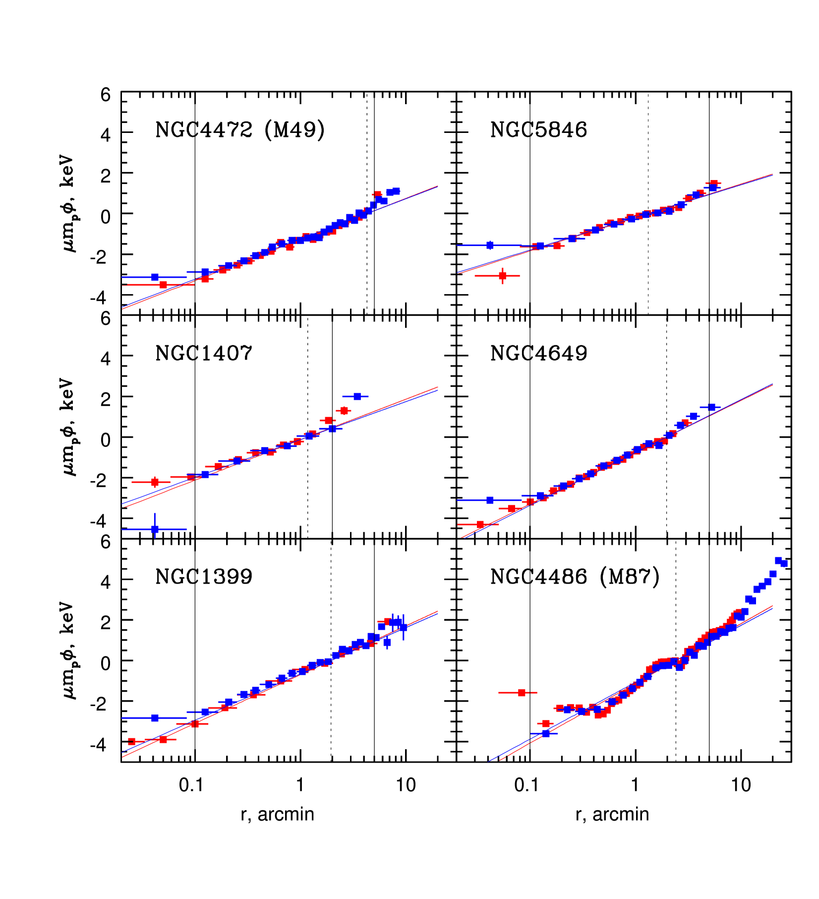
Figure 1: Gravitational potentials derived from Chandra (red) and XMM-Newton/MOS (blue) observations of each galaxy. Potentials are normalized to zero at $R_{e}$. Vertical lines mark the range of radii used to approximate the data by a $v_{c}^{2}\log r+b$ law, and the thin solid lines are the best-fit approximations of the Chandra and XMM-Newton data to this law. The vertical dotted lines mark the effective radius.

As discussed in C08 the expression (2) for the potential can be evaluated directly from deprojected data - density and temperature profiles. Since the logarithmic derivative of the density $\frac{d\log n}{dr}$ is under the integral the enhancement of errors due to differentiation is not a major issue and evaluation of eq. (2) does not require any parametric description of the density and/or temperature profiles. This removes the ambiguity in the choice of a functional form for these profiles. Since the potential is calculated directly via eq. (2) no apriori parametrization of the potential (or mass) is required. If information on the gravitational potential is available from other data (e.g. from optical observations) the comparison of the potential profiles can be done directly with the results of eq. (2). In C08 the relation between potential profiles derived from X-ray and optical data was written as $\varphi_{X}=a\varphi_{opt}+b$ and the value of $a$ was evaluated. In this case any transformation of the potential profile to the circular speed (or equivalently to the mass profile) which involves differentiation of the potential profile is not needed and should be avoided.

Thus, the application of eq. (2) to the X-ray data is essentially free from any parametrization and does not rely on direct differentiation of the data. This is the main difference with most of the other techniques which either use parametrization of the density/temperature profiles or make an assumption on the form of the mass profile (see e.g. Mathews, 1978; Fabian et al., 1981; Forman, Jones, & Tucker, 1985; Nulsen & Bohringer, 1995; Humphrey et al., 2006; Fukazawa et al., 2006, for various techniques of the mass profile reconstruction). The most close approach to ours is that of Humphrey et al. (2006), where the temperature and mass profiles are parametrized, the hydrostatic equilibrium equation is solved to find the density and the best-fitting parameters are iteratively found. As mentioned above in eq. (2) all observables are on the r.h.s and one can reconstruct the potential directly and defer the parametrization (if needed) to a final step of manipulations with reconstructed potential.

We are now considering the case when limited information on the potential from optical data is available. For instance, consider a situation when only central velocity dispersion of the galaxy is known (see discussion in §3). In this case to compare X-ray and optical potentials a parametrization of the potential derived from eq. (2) is needed. An especially simple and straightforward parametrization is possible if the potential is isothermal $\varphi=v^{2}_{c}\log r+b$, since in this case a single number – circular speed $v_{c}$ can characterize the potential. In fact, recent studies using stellar kinematics and lensing do suggest that the potentials of early-type galaxies are approximately isothermal (Gerhard et al., 2001; Treu et al., 2006; Gavazzi et al., 2007), similar to disk galaxies. Consistency of the mass profile with $M(r)\propto r$ (implying an isothermal potential) was also suggested for several elliptical galaxies based on the analysis of X-Ray data (e.g., Trinchieri & Fabbiano, 1985; Buote & Canizares, 1994; Kim & Fabbiano, 1995; Nulsen & Bohringer, 1995; Buote & Canizares, 1998; Fukazawa et al., 2006). Below we confirm an approximate isothermality of the potentials using the results of application of the non-parametric method (eq. 2) and determine the best-fitting value of $v_{c}$.

The axes in Figure 1 are log-linear and therefore an isothermal (logarithmic) potential should look like a straight line $v^{2}_{c}\log r+b$. To first order this is true, although there are statistically significant deviations, particularly at the innermost and outermost radii, which we discuss below. The agreement of Chandra and XMM-Newton data is good, except for the inner region where the better spatial resolution of Chandra is important. We choose to ignore the data inside the $r_{1}=0.1^{\prime}$ circle where this effect is apparent. We also introduce a cutoff at large radii (typically $r_{2}\approx 5^{\prime}$), where the results are sensitive to the assumed extrapolation of the emissivity profile. The actual values of $r_{1}$ and $r_{2}$ used in the analysis are given in Table 2 and are shown in Figure 1 as a pair of vertical lines. Between $r_{1}$ and $r_{2}$ the potential was approximated with a logarithmic function $v_{c}^{2}\log r+b$ with $v_{c}$ and $b$ being free parameters. Best fitting values were found by minimizing the root-mean-square deviation between the model and observed potential profiles. The resulting values of $v_{c,X}$ for Chandra and XMM-Newton data are given in Table 2 as $v_{c,\rm Chandra}$ and $v_{c,\rm XMM}$. The statistical uncertainties determined from the Monte Carlo procedure are also given in Table 2. In general there is good agreement between the values obtained by the two instruments, confirming that the uncertainties introduced by statistical errors and cross-calibration uncertainties between the two instruments (including background subtraction procedures) are small. One can expect however that the real uncertainties are dominated by systematic errors arising from our model assumptions (e.g., the assumption of spherical symmetry used in the deprojection analysis), which affect both datasets in similar ways. For subsequent analysis we use the average of the results from the two instruments, $v_{c,X}\equiv(v_{c,\rm Chandra}+v_{c,\rm XMM})/2$ (last column in Table 2).

The deviations of the potential from the isothermal shape $\varphi=a\log r+b$ can be studied by assuming a functional form $\varphi=ar^{\alpha}+b$ and looking for the best-fitting value of $\alpha$. For the five galaxies with $r_{1}=0.1^{\prime}$ and $r_{2}=5^{\prime}$ the best-fitting value of $\alpha$ varies from $0.03$ for NGC1399 to $0.16$ for NGC4472 (the mean value of $\alpha$ is 0.11). For NGC1407 ($r_{1}=0.1^{\prime}$ and $r_{2}=2^{\prime}$) the value of $\alpha$ is $\sim 0.5$. This suggests that on average the profiles are slightly concave, i.e. circular speed slightly increases at large radii, which can be seen in Fig. 1. This is consistent with the fact that these massive ellipticals are sitting at the centers of more massive group/cluster size halos which dominate at large radii. Given the mean value of $\alpha=0.11$ one can estimate that changing both $r_{1}$ and $r_{2}$ by a factor of two would on average change the estimate of $v_{c}$ by a factor of only $\displaystyle 2^{\alpha/2}\sim 4$%.

We explicitly tested the sensitivity of $v_{c}$ to the values of $r_{1}$ and $r_{2}$ for all objects in the sample by increasing the lower boundary by a factor of two (i.e. $r_{1}=0.2^{\prime}$) and recalculating $v_{c}$. The results of this test are given in Table 3 (column $\Delta_{\rm r_{1}\times 2}$), where

$$\Delta_{\rm r_{1}\times 2}=\frac{v_{c,{\rm r_{1}\times 2}}-v_{c,X}}{v_{c,X}},$$ (3)

and $v_{c,X}$ is the circular speed from Table 2, and $v_{c,{\rm r_{1}\times 2}}$ is calculated as a mean value of circular speeds measured using Chandra and XMM-Newton for increased $r_{1}$ (similarly to $v_{c,X}$ in Table 2). In a separated test we decreased the value of $r_{2}$ by a factor of two (i.e. $r_{2}=2.5^{\prime}$ for all objects except for NGC1407, where $r_{2}=1^{\prime}$) and again recalculated $v_{c}$ (see Table 3, column $\Delta_{\rm r_{2}/2}$). From Table 3 it follows that factor of 2 changes in either $r_{1}$ or $r_{2}$ causes few per cent changes in $v_{c}$.

2.1 Flat abundance profile

We now illustrate the impact of our assumption of a flat abundance profile, using NGC1399 as an example.

As is obvious from equation (2), the absolute normalization of the gas density $n$ does not affect the calculations of the potential. From this point of view it is not the particular value of the heavy-element abundance in the spectral models, but rather the radial variation of the abundance that affects the derived potential profile. In elliptical galaxies one can expect an increase of metal abundance towards the center of the galaxy. This is usually true for a range of radii except for the very center, where a “dip” in the metal abundance is often seen when fitting the data with a single temperature plasma emission model (e.g., Matsushita et al., 2002).

As mentioned above, measuring the metal abundance from X-ray spectra in cool systems is difficult because of the ambiguity of separating line from continuum emission with the limited energy resolution of X-ray CCDs. For a multi-temperature plasma this separation is even more complicated because fitting the emission with one-temperature models leads to a biased estimate of the abundance (e.g., Buote, 2000). In deprojected spectra, such as we use here, the bias arising from a multi-temperature plasma is reduced because the superposition of cooler and hotter emission coming from different radii is removed (provided the object is spherically symmetric), although if the plasma is intrinsically multi-temperature then the problem remains. On the other hand the signal-to-noise of the deprojected spectra is much lower than for the projected spectra. It is therefore desirable to keep the number of free parameters in the fit as small as possible.

As an example we show in Figure 2 (left) the gas parameters (electron density, temperature and abundance of heavy metals) as a function of radius for NGC1399. In two models (blue circles and green triangles) the abundance was fixed at 0.5 and 1 times solar, respectively. In the third model (red squares) the abundance was a free parameter. One can see that in the third model the errors on the abundance are substantial and, as expected, the abundance and the gas density are anti-correlated. The potential profiles corresponding to these spectral models are shown in the right panel of Figure 2. Clearly there is a significant change in the potential curves (curves are normalized to zero potential at $1^{\prime}.5$). Formally calculated values of $v_{c}$ for the three spectral models are:

$$\begin{array}[]{ll}v_{c}&=421~{}\,{\rm km~{}s}^{-1};\hbox{ free abundance}\\ v_{c}&=403~{}\,{\rm km~{}s}^{-1};\hbox{ abundance$\,=0.5\ \times$ solar}\\ v_{c}&=396~{}\,{\rm km~{}s}^{-1};\hbox{ abundance$\,=1\ \times$ solar}.\\ \end{array}$$ (7)

Thus, there is a substantial, but not dramatic effect of the assumed abundance profile on the derived logarithmic slope of the potential profile. Given that the limited statistics in our deprojected spectra do not allow for a robust abundance determination for all galaxies in the sample, we decided to keep the assumption of a flat abundance profile so that we could analyze all objects in a uniform way. It is likely that this approximation introduces errors in the best-fitting value of $v_{c}$ of roughly 5-15$\,{\rm km~{}s}^{-1}$. If all galaxies in our sample have a similar abundance profile to the one derived in NGC1399, one can expect the values of $v_{c}$ obtained under the assumption of a flat profile with $0.5\ \times$ solar metallicity to be biased low by  3-4%.

Relative changes in the circular speed when abundance of heavy elements is a free parameter (constrained to be in the range from 0 to 2) for all objects in the sample are calculated in Table 3 (column $\Delta_{\rm abund}$):

$$\Delta_{\rm abund}=\frac{v_{c,{\rm free~{}abundance}}-v_{c,{X}}}{v_{c,{X}}},$$ (8)

where $v_{c,{\rm free~{}abundance}}$ is calculated as a mean value of circular speeds measured using Chandra and XMM-Newton, similarly to $v_{c,X}$ (see §2).

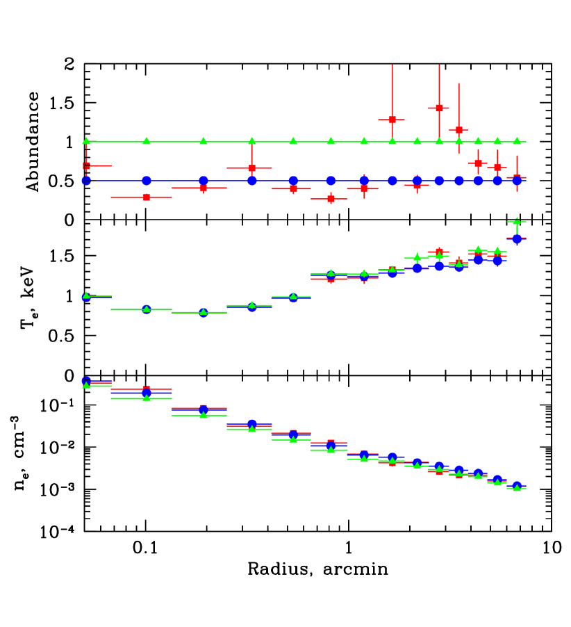
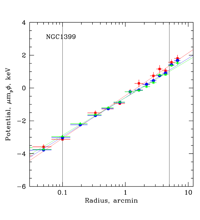
Figure 2: Left: Radial profiles of deprojected gas parameters (abundance, temperature, electron density) in NGC1399. The parameters were obtained using a single-temperature APEC model (with fixed low-energy absorption and redshift) fit to the deprojected Chandra spectra from a set of spherical shells. For the blue and green models (circles and triangles) the abundance was fixed at 0.5 and 1 times solar, respectively, while for the red model (squares) the abundance was a free function of the radius. Right: Potential profiles corresponding to the spectral models shown in the left panel. Straight lines show best-fitting approximations $\varphi=v_{c}^{2}\log r+b$.

Yet another parameter related to the chemical composition of the hot gas that is important for the evaluation of the gravitational potential is the mean atomic weight $\mu$ (see eq. 2). For the solar photospheric abundance table of Anders & Grevesse (1989) $\mu=0.614$ (assuming fully ionized plasma). If we lower the abundance of heavy elements to 0.5 solar, $\mu$ changes to 0.610, i.e. by 0.7%. Changing the helium abundance would, of course, have a much stronger impact on $\mu$. For instance, doubling the abundance of helium relative to the solar photospheric mix would increase $\mu$ to 0.695, i.e., by 13%. One mechanism that could lead to helium enrichment beyond solar abundance is gravitational sedimentation of heavy elements (e.g., Gilfanov & Sunyaev, 1984; Chuzhoy & Nusser, 2003; Chuzhoy & Loeb, 2004; Ettori & Fabian, 2006). If sedimentation is indeed important for the interstellar gas in the cores of elliptical galaxies, then it will also affect the emissivity. In the present work we assume that $\mu={\rm const}=0.61$ at all radii, but one should bear in mind that the results might change if the helium abundance changes with radius or simply differs from the canonical value of $7.92\times 10^{-2}$ (number density relative to hydrogen) adopted here.

2.2 Deviations from spherical symmetry

To make a crude estimate of an impact on $v_{c}$ by possible deviations from spherical symmetry one can make deprojection analysis in individual wedges and compare the results. We divided the data on each object into two independent halves - Northern and Southern and repeated the analysis for each half separately. The difference in the circular speeds between two halves is given in Table 3 (column $\Delta_{\rm NS}$):

$$\Delta_{\rm NS}=\frac{v_{c,{N}}-v_{c,{S}}}{v_{c,{X}}},$$ (9)

where $v_{c,N}$ and $v_{c,S}$ are the circular speeds for the Northern and Southern halves respectively. For most of the objects the difference is at the level of 2-4% (compared to $\sim$1% pure statistical uncertainty).

The largest difference $\sim$8% is for NGC1407. Inspection of the data have shown that this difference primarily comes from XMM-Newton data. We note that NGC1407 was observed by XMM-Newton with an offset angle of $\sim 8^{\prime}$ and the PSF distortions might contribute to this difference.

In the analysis of optical data (§3) we discuss optical constraints on the gravitational potential, assuming that the galaxies are spherically symmetric. All objects in the sample are round, being E0-E2 galaxies, although in some objects (e.g. M87) the ellipticity increases with radius. We note here that in the radial range where stars are dominating the mass, the potential is more spherical than the distribution of the stars themselves. The same is likely true even in outer regions, given a steep decrease ($R^{-2}$ or steeper) of the optical surface brightness.

The analysis of independent wedges is not a useful indicator of a possible error in the effective circular speed when the object posses an axial symmetry and is viewed pole-on. Possible effects of a non-spherical potential on optical estimates for a pole-on galaxy are discussed in C08 (Section 7.2 there). There we show that for an axis ratios (along and perpendicular to the line-of-sight) of 0.5 (oblate) and 2 (prolate) the error in mass is factor of 0.79 and 1.04 respectively, and argue that the probability that many objects in our sample are strongly oblate or oblate systems viewed pole-on is rather low. Therefore on average the error is going to be smaller than these extreme values.

X-ray analysis of the ellipsoidal objects is discussed in Piffaretti, Jetzer, & Schindler 2003 and C08. If potential is logarithmic and the isothermal gas is in hydrostatic equilibrium, then the potential is recovered correctly from the spherically symmetric analysis (see Appendix B in C08). For a more complicated potential or non-isothermal gas the deviations are present (see e.g. Fig.1 in Piffaretti, Jetzer, & Schindler, 2003, for an example of expected bias for prolate and oblate cases in A2390 cluster). Although the effects of non-spherical potential are different for X-ray and optical analysis, the sign of the effect for oblate and prolate systems is the same. Therefore errors in mass/potential partly compensate each other when effective circular speeds are compared.

We concluded that the assumption of a spherical potential can contribute to the discrepancy between X-ray and optical data, but it is unlikely that on average the magnitude of the effect exceeds several per cent.

2.3 Contribution of unresolved LMXBs and weak sources

The contribution of low-mass X-ray binaries (LMXB) can dominate the X-ray emission in gas-poor elliptical galaxies (e.g., Trinchieri & Fabbiano, 1985). Even when the spatial resolution and sensitivity allows the resolution of some LMXBs the remaining emission can still be dominated by even weaker unresolved sources, such as accreting white dwarfs (see, e.g., Revnivtsev et al., 2008, for the analysis of the galaxy NGC3379).

Since all objects in our sample are gas-rich galaxies the contribution of unresolved sources is not a major issue, especially for such bright objects as M87 and NGC1399. For less luminous objects, because of their harder spectrum compared to the hot gas emission, LMXBs can affect the observed fluxes at the high end of the Chandra and XMM-Newton energy bands. To test the magnitude of this effect we added a power law component with a photon index $\Gamma=1.6$ with a free normalization to represent the contribution of unresolved sources (e.g., Irwin, Athey, & Bregman, 2003; David et al., 2006; Humphrey & Buote, 2006) and recalculated the circular speed for NGC4472. The resulting values are only $\sim$1% lower than in Table 2.

Relative changes in the circular speed when a power law component with a photon index $\Gamma=1.6$ is added to the spectral model for all objects in the sample are calculated in Table 3 (column $\Delta_{\rm LMXB}$):

$$\Delta_{\rm LMXB}=\frac{v_{c,{\rm LMXB}}-v_{c,{X}}}{v_{c,{X}}}.$$ (10)

On average adding a power law component shifts the circular speed few percent lower. The largest effect is for M87 and in this very gas rich galaxy the change in $v_{c}$ likely reflects the complexity of the spectrum rather then the contribution of real LMXBs.

2.4 Summary on uncertainties in X-ray analysis

The summary of the uncertainties in determination of the circular speed from X-ray data is given in Table 3. The columns in the table show the relative deviation of the circular speed from the reference value $v_{c,{X}}$ given in Table 2 when changes are made to the analysis procedure. The quoted uncertainties in columns labeled Ërr.äre pure statistical errors. They have clear meaning only when the difference between the Northern and Southern parts of the galaxies are considered, since the data are independent. In all other cases the quoted uncertainty corresponds to the largest statistical error in one of the two values of $v_{c}$ used to calculate $\Delta$.

The last two rows in the Table 3 give the mean change in the circular speed and the RMS value (relative to zero). The values given in the Table allows one to get an idea of the uncertainties introduced by the assumptions incorporated into calculations of $v_{c}$. For instance, letting abundance be a free parameter on average shifts the value of $v_{c}$ up by $\sim 2$%, while adding a power law component (to control possible contribution of LMXBs) on the contrary shifts $v_{c}$ down by $\sim 2$%. Changing any of the bounds of the fitting range $r_{1}$ and $r_{2}$ by a factor of 2 changes $v_{c}$ by few % up or down.

While rigorous evaluation of combined uncertainties is difficult, we can very crudely estimate it by adding RMS values of $\Delta_{\rm abund}$, $\Delta_{\rm LMXB}$, $\Delta_{\rm NS}$, $\Delta_{\rm r1}$ and $\Delta_{\rm r2}$ quadratically. The resulting value 7.1% is crude a characteristic of the uncertainties in the final value of $v_{c,X}$ introduced by the modifications of our analysis procedure. Note that pure statistical errors also contribute to the above estimate.

Table 3: Relative changes in circular speed with respect to the reference value $v_{c,{X}}$ given in Table 2 when changes are made to the analysis procedure (see §2.4).

Galaxy	$\Delta_{\rm abund}$	Err.	$\Delta_{\rm LMXB}$	Err.	$\Delta_{\rm NS}$	Err.	$\Delta_{\rm r_{1}\times 2}$	Err.	$\Delta_{\rm r_{2}/2}$	Err.
	%		%		%		%		%
ngc1399	4.23	0.80	-2.01	0.44	2.36	0.64	1.40	0.94	1.22	0.39
ngc1407	0.76	5.67	-1.61	2.37	8.25	2.88	5.66	1.74	1.05	2.22
ngc4472	2.43	2.17	-0.98	0.79	-2.31	1.16	-0.42	0.76	-3.71	0.70
ngc4486	3.88	0.40	-5.69	0.37	-4.58	0.39	1.44	0.26	-1.00	0.31
ngc4649	-2.48	1.14	0.36	0.41	2.67	0.62	3.30	0.43	0.08	0.39
ngc5846	1.53	2.61	-1.82	1.02	-2.57	1.50	-1.68	0.81	-5.14	1.21
Mean	1.73		-1.96		0.64		1.62		-1.25
RMS	2.82		2.69		4.35		2.89		2.70

Name	changes in the analysis	Section
$\Delta_{\rm abund}$	free metal abundance	(§2.1)
$\Delta_{\rm LMXB}$	a power law is added	(§2.3)
$\Delta_{\rm NS}$	difference between North and South	(§2.2)
$\Delta_{\rm r1}$	$r_{1}\times 2$	(§2)
$\Delta_{\rm r2}$	$r_{2}/2$	(§2)

3 Robust estimators of the isothermal potential from optical data

The results of the X-ray analysis suggest that the shape of the potential profile of the galaxies in our sample is not far from isothermal over the range of radii $\sim 0.5$–25 kpc, corresponding to $\sim 0.05$–$3~{}R_{e}$. Let us assume that this is true at all radii and the total gravitational potential of a galaxy is logarithmic,

$$\varphi(r)=v_{c}^{2}\log r+{\rm const.}$$ (11)

It is natural to ask, given this assumption, how the velocity dispersion of the stars in the galaxy is expected to be related to $v_{c}$. A robust method to determine $v_{c}$ from optical observations would enable us to check our results by comparing the derived values in Table 2, to determine $v_{c}$ and thus the gravitational potential for many galaxies without X-ray observations, and to look for evidence of non-thermal pressure support in the X-ray gas.

For simplicity we shall assume that the galaxy is spherical with known surface brightness $I(R)$ and line-of-sight velocity dispersion $\sigma(R)$, and ask what is the best way to determine $v_{c}$ from known $I(R)$, $\sigma(R)$ given that the potential is isothermal.

3.1 Circular speed from velocity dispersion for distant (unresolved) galaxies

Since the acceleration of a star in the logarithmic potential $\ddot{\mathbf{r}}=-\mbox{\boldmath$\nabla$}\varphi=v_{c}^{2}{\mathbf{r}}/r^{2}$, the virial theorem for such a system reads

$$0=\left<\dot{{\mathbf{r}}}^{2}+{\mathbf{r}}\cdot\ddot{\mathbf{r}}\right>=\left<{\mathbf{v}}^{2}\right>-v_{c}^{2},$$ (12)

where ${\mathbf{v}}=\dot{{\mathbf{r}}}$. Since the galaxy is spherical, the mean-square velocity along any line of sight is equal to $\frac{1}{3}\langle{\mathbf{v}}^{2}\rangle$ and therefore

$$v_{c}^{2}=3\,\frac{\int_{0}^{\infty}dRR\,I(R)\sigma^{2}(R)}{\int_{0}^{\infty}dR\,RI(R)},$$ (13)

i.e., the circular speed is equal to $\surd{3}$ times the integrated line-of-sight dispersion for the whole galaxy. This formula is useful for distant (unresolved) galaxies that lie entirely within the spectrograph slit, or within the field of an integral-field spectrograph. For nearby galaxies, however, this formula is not useful since velocity-dispersion profiles typically go out only to the effective radius $R_{e}$ (eq. 17), which contains only half the light.

3.2 Circular speed from velocity dispersion for Sérsic models

3.2.1 Constant anisotropy

Figure 3: Line-of-sight velocity dispersion as a function of radius for spherical galaxy models with Sérsic index $n=1,4,12$ – left, middle, right panels respectively. The solid, dotted and dashed lines correspond to systems composed of isotropic, circular and radial stellar orbits. The thin vertical line shows the position of the “optimal radius” or “sweet spot” at which the deviations among the three models are minimized.

Let us continue to assume that we have a spherical galaxy in a logarithmic potential and consider three variants of the stellar orbital anisotropy: isotropic orbits (i.e., the velocity-dispersion tensor is isotropic), circular orbits, and radial orbits. It is straightforward to show from the Jeans equation (see Appendix A) that the line-of-sight velocity dispersion in these three models is given by:

$$\sigma^{2}(R)=\sigma_{\rm iso}^{2}(R)\equiv v^{2}_{c}\frac{R}{I(R)}\int_{R}^{\infty}\frac{I(x)}{x^{2}}dx,$$ (14)

for isotropic orbits,

$$\sigma^{2}(R)=\sigma_{\rm circ}^{2}(R)\equiv\frac{1}{2}\left[v^{2}_{c}-\sigma_{\rm iso}^{2}(R)\right],$$ (15)

for circular orbits and

$$\sigma^{2}(R)=\sigma_{\rm rad}^{2}(R)\equiv\frac{1}{2}v^{2}_{c}\frac{1}{RI(R)}\int_{R}^{\infty}I(x)\left(1-R^{2}/x^{2}\right)dx,$$ (16)

for pure radial orbits. In Figure 3 the radial dependence of the line-of-sight velocity dispersion is shown for the above three cases, assuming that the surface brightness of the galaxy is described by a Sérsic law $I(R)\propto\exp(-aR^{1/n})$ with index $n=1,4,12$. The radius is plotted in units of the effective radius $R_{e}$, the radius containing half the light:

$$\int_{0}^{R_{e}}RI(R)dR=\frac{1}{2}\int_{0}^{\infty}RI(R)dR.$$ (17)

From Figure 3 it is clear that for all $n$ and for all three models spanning the range of possible anisotropies the dispersions are rather similar at about 0.5–$0.6R_{e}$. This result suggests that somewhere near this radius the line-of-sight velocity dispersion may provide a measure of the circular speed of the underlying isothermal potential that is relatively independent of the details of the stellar velocity distribution.

There are many possible ways to define the “optimal” radius or “sweet spot” at which the relation between the line-of-sight velocity dispersion and the circular speed is likely to exhibit the smallest variation. In Figure 4 we plot the radii where the line-of-sight dispersions from each pair of the three models coincide, as a function of Sérsic index $n$. From equations (14), (15) and (16) these are the solutions of the equations

$$\begin{array}[]{ll}n\Gamma(n,z)=z^{n}e^{-z}&{\rm circular=radial}\\ 3z^{n}n\Gamma(-n,z)=e^{-z}&{\rm isotropic=circular}\\ 3z^{2n}\Gamma(-n,z)=\Gamma(n,z)&{\rm isotropic=radial},\end{array}$$ (18)

where $z=aR_{s}^{1/n}$, and $\Gamma$ is the upper incomplete gamma function. Models of galaxy formation usually suggest that the velocity-dispersion tensor is isotropic near the center and radially biased ($\sigma_{r}^{2}>\sigma_{\theta}^{2}$) in the outer parts of the galaxy, so we should prefer the bottom half of the range of $R_{s}$ indicated by these curves. A natural choice for the sweet spot $R_{s}$ is the middle curve, where the line-of-sight velocity dispersions for radial and circular models are equal (thin vertical lines in Figure 3). This can be written for arbitrary surface-brightness profiles as

$$\int_{R_{s}}^{\infty}I(x)dx=R_{s}I(R_{s}).$$ (19)

The values of $R_{s}$, $\sigma_{\rm iso}(R_{s})$, $\sigma_{\rm circ}(R_{s})$ and $\sigma_{\rm rad}(R_{s})$ (the latter two quantities coincide by the definition of $R_{s}$) are shown in Figure 5 and in Table 4, as a function of $R_{s}/R_{e}$.

Figure 4: Radius $R_{s}(n)$ at which the line-of-sight dispersions (eqs. 14, 15, and 16) for systems composed from different types of orbits coincide, as a function of Sérsic index $n$. Solid line: $\sigma_{\rm circ}(R)=\sigma_{\rm rad}(R)$, dashed line: $\sigma_{\rm iso}(R)=\sigma_{\rm rad}(R)$, dotted line: $\sigma_{\rm iso}(R)=\sigma_{\rm circ}(R)$.

Figure 5: The line-of-sight dispersions evaluated at $R_{s}(n)$ [where $\sigma_{\rm circ}(R_{s})=\sigma_{\rm rad}(R_{s})$] are shown with solid (for systems with intrinsically isotropic orbits) and dashed (radial and circular orbits) lines.

The range of dispersions spanned by these three models is of course smaller than the range spanned by all possible equilibrium models (see for example Figures 1 and 2 of Richstone & Tremaine 1984). Our results nevertheless suggest that the line-of-sight velocity dispersion evaluated at $R_{s}\simeq 0.5R_{e}$ is a better proxy for the circular speed in a galaxy with a logarithmic potential than the dispersion at any other radius (e.g., the central velocity dispersion).

Determination of the effective radius and the Sérsic index of real galaxies depends (sometimes strongly) on the range of radii used to fit the surface brightness profile and on the method of extrapolating to calculate the total flux. This is especially true for galaxies with extended envelopes, characteristic of central galaxies in clusters and groups. For such galaxies the reported values of $R_{e}$ and $n$ for the same object may vary strongly. A striking example is M87: the effective radius of $145^{\prime\prime}$ in Table 1 (D’Onofrio, Capaccioli, & Caon, 1994) is a factor of almost five smaller than the most recent value $R_{e}=704^{\prime\prime}$ in Kormendy et al. (2009). Similarly the reported values of the Sérsic index vary from 6.51 in D’Onofrio, Capaccioli, & Caon (1994) to 11.84 in Kormendy et al. (2009). The position of the sweet spot changes accordingly. Clearly such large variations have two main causes: (i) deviations of the observed surface-brightness profile from a pure Sérsic profile, and (ii) the weak dependence of the surface-brightness slope on $R/R_{e}$ and $n$ or, more precisely, strong covariance between $R_{e}$ and $n$ when fitting to data. Indeed for the Sérsic profile the slope is (e.g., Graham & Driver, 2005)

$$-\frac{d\log I(R)}{d\log R}\approx 2\left(\frac{R}{R_{e}}\right)^{1/n}.$$ (20)

Obviously when $n$ is large the variations of slope at a given $R$ are not very sensitive to the variations of $R_{e}$.

This raises the question of which set of $n$ and $R_{e}$ to use and how strongly the final result (circular speed evaluated near the sweet spot) depends on these parameters. The definition of the sweet spot (eq. 19) does not explicitly use the value of $R_{e}$, but is instead most sensitive to the slope of the surface brightness profile; thus, for example, if $I(R)\propto R^{-2}$ for $R>R_{0}$ then any radius $R>R_{0}$ can equally well serve as the sweet point (see also §3.3). This implies that the evaluated circular speed should not be sensitive to the precise values of $R_{e}$ and $n$ so long as they provide a good fit to the surface-brightness profile and our other assumptions (e.g., circular speed independent of radius) are satisfied.

To illustrate this point, let us assume that M87 has circular speed independent of radius, isotropic velocity-dispersion tensor, and surface-brightness profile that is accurately fit by a Sérsic profile with the Kormendy et al. parameters, $R_{e}=704^{\prime\prime}$ and $n=11.84$, and that we estimate the circular speed using Table 4 and the D’Onofrio et al. parameters $R_{e}=145"$ and $n=6.51$. The resulting error in $v_{c}$ will be only 3% even though the values of $R_{e}$ differ by a factor of almost five.

In practice the sweet spot at large radius is less favorable since measurements of the line-of-sight velocity dispersion have only a limited radial extent. In particular, to estimate the circular speed using the effective radius from Kormendy et al. one needs the stellar velocity dispersion at a radius of $\sim 0.5R_{e}\sim 5$–$6^{\prime}$, which is not known. For this reason we decided to use the effective $R_{e}=145^{\prime\prime}$ of D’Onofrio et al.

It is possible that equation 19 does not have roots at radii where good measurements of the line-of-sight velocity dispersion are available. In this case one can look for the radius $R$ with measured $\sigma(R)$ where the relative mismatch of the left and right sides of equation 19 is smallest.

In the limit of large Sérsic index $n$, the surface brightness of a galaxy at radii not too far from the effective radius declines as $R^{-2}$ (e.g., Graham & Driver, 2005) and therefore volume emissivity declines as $r^{-3}$. While formally the total mass and the effective radius diverge as $n$ goes to infinity, at the same time the line-of-sight velocity dispersion becomes independent of the radius and the anisotropy of stellar orbits (Gerhard, 1993) as long as the shape of the velocity-dispersion tensor, $\sigma_{\theta}^{2}/\sigma_{r}^{2}$, does not depend on radius. In this limit $\sigma^{2}(R)={\rm const}=v^{2}_{c}/3$ at all radii (Table 4).

Table 4: Dependence of $R_{s}$ and line-of-sight velocity dispersions at $R_{s}$ on the Sérsic index $n$. Here $R_{s}$ is such that $\sigma_{\rm circ}(R)=\sigma_{\rm rad}(R)$; $R_{s}$ is measured in units of the effective radius $R_{e}$, and $\sigma$ is measured in units of the circular speed $v_{c}$.

$n$	$R_{s}/R_{e}$	$\sigma_{\rm iso}$	$\sigma_{\rm circ}=\sigma_{\rm rad}$	$(\sigma_{\rm iso}-\sigma_{\rm circ})/\sigma_{\rm iso}$
1	0.595824	0.635337	0.546053	0.140530
2	0.553551	0.615010	0.557567	0.0934008
3	0.530947	0.605640	0.562672	0.0709465
4	0.516328	0.600140	0.565611	0.0575356
5	0.505918	0.596490	0.567538	0.0485364
6	0.498051	0.593877	0.568907	0.0420463
7	0.491859	0.591909	0.569932	0.0371287
8	0.486838	0.590369	0.570730	0.0332661
9	0.482674	0.589130	0.571369	0.0301473
10	0.479156	0.588111	0.571894	0.0275738
11	0.476140	0.587256	0.572333	0.0254124
12	0.473523	0.586530	0.572705	0.0235703
13	0.471228	0.585904	0.573025	0.0219810
14	0.469199	0.585359	0.573304	0.0205953
15	0.467389	0.584881	0.573548	0.0193760
16	0.465765	0.584457	0.573764	0.0182946
17	0.464299	0.584078	0.573957	0.0173289
18	0.462968	0.583738	0.574130	0.0164609
19	0.461754	0.583432	0.574285	0.0156766
20	0.460642	0.583153	0.574427	0.0149643
$\infty$	$\infty$	0.577350	0.577350	0

3.2.2 Anisotropy changing with radius

In the models considered above the anisotropy parameter was independent of radius. We now consider several simple models in which anisotropy parameter $\beta(r)=1-\sigma_{\theta}^{2}(r)/\sigma_{r}^{2}(r)$ depends on radius according to

$$\beta(r)=\frac{\beta_{2}r^{c}+\beta_{1}r_{a}^{c}}{r^{c}+r_{a}^{c}~{}},$$ (21)

where $\beta_{1}$ and $\beta_{2}$ are the anisotropy parameters at $r=0$ and $r\to\infty$ respectively, $r_{a}$ is the anisotropy radius, and the exponent $c$ controls the sharpness of the transition. The radial velocity dispersion is then

$$\sigma_{r}^{2}(r)=\frac{v_{c}^{2}}{j(r)W(r)}\int_{r}^{\infty}\frac{j(x)W(x)}{x}dx,$$ (22)

where

$$W(x)=x^{2\beta_{1}}(x^{c}+r_{a}^{c})^{2(\beta_{2}-\beta_{1})/c}.$$ (23)

A similar model with $c=1$, $\beta_{1}=0.2$, $\beta_{2}=1$ was used to describe the anisotropy profile in M87 by Doherty et al. (2009). Another special case of our parametrization is the Osipkov–Merritt model (Osipkov, 1979; Merritt, 1985), corresponding to $c=2$, $\beta_{1}=0$, $\beta_{2}=1$.

In the left panel of Figure 6 we show the behavior of the anisotropy parameter $\beta$ for $c=1,2$ and 4 and different values of the anisotropy radius $r_{a}$. The Doherty et al. models ($c=1$) are shown by black lines and the Osipkov-Merritt models ($c=2$) by red lines, both for $r_{a}=0.1R_{e}$, $1R_{e}$, $5R_{e}$. In the right panel of Figure 6 we show corresponding profiles of line-of-sight velocity dispersion for an $n=4$ Sérsic model. The legends of the lines are the same as in the left panel. For reference, the thick green lines show our standard isotropic, circular and radial models.

We did not check explicitly that these solutions of the Jeans equation correspond to non-negative distribution functions. Sérsic models with $\beta=1$, corresponding to purely radial orbits, certainly have negative distribution functions and thus are unphysical. For the Osipkov–Merritt models, the smallest anisotropy radius shown in Figure 6 is $r_{a}=0.1R_{e}$, close to but outside the range $r_{a}\lesssim 0.05R_{e}$ at which the distribution function is negative (Merritt, 1985).

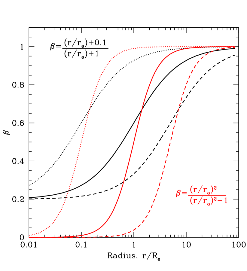
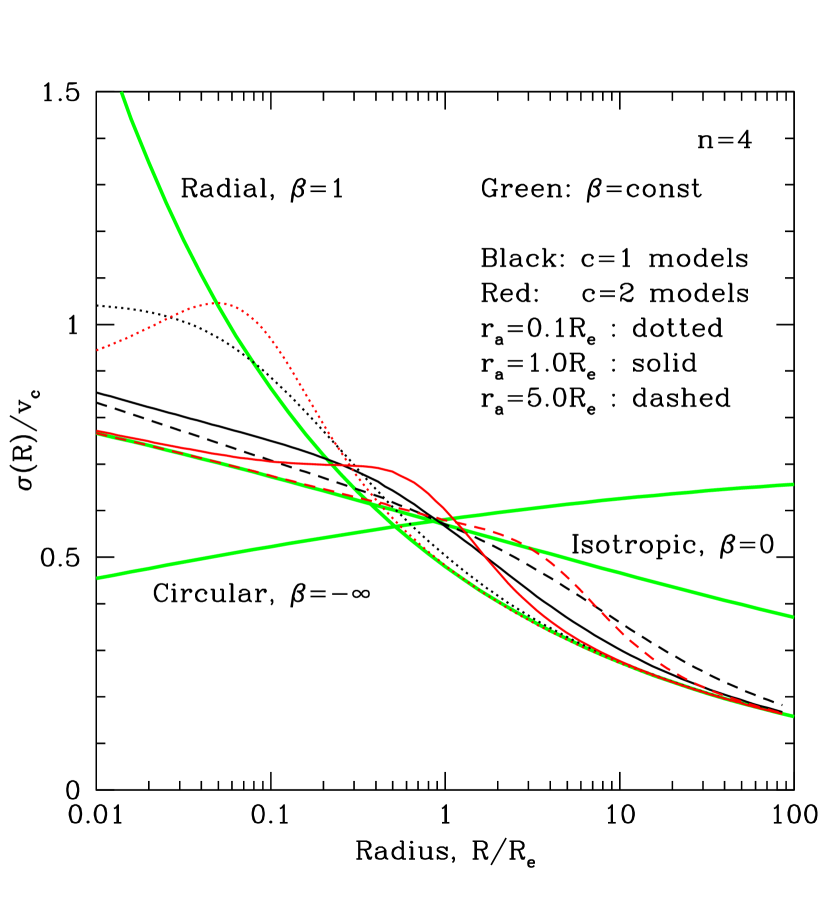
Figure 6: Left: Radial dependence of the anisotropy parameter $\beta$. The Doherty et al. models ($c=1$) are shown by black lines, and the Osipkov-Merritt models ($c=2$) by red lines. The curves corresponding to different values of the anisotropy parameter $r_{a}$ (see eq. 21) are shown with dotted, solid and dashed lines for $r_{a}=0.1R_{e}$, $1R_{e}$ and $5R_{e}$ respectively. Right: Corresponding profiles of line-of-sight velocity dispersion for an $n=4$ Sérsic model. The legends of the lines are the same as in the left panel. The thick green lines show for reference our standard isotropic, circular and radial models.

Considering the models shown in the right panel of Figure 6 it is clear that the “sweet spot” at which the sensitivity of the line-of-sight dispersion to the orbit structure is minimized is near $0.5R_{e}$, just as we found in §3.2.1 from examining models with radial, circular, and isotropic orbits. However, and not surprisingly, the models with radially varying anisotropy span a larger range in line-of-sight dispersion at the sweet spot, with the largest deviations occurring when $r_{a}/R_{e}\sim 1$. For instance at $R=0.516R_{e}$ (taken from Table 4 for $n=4$) the Osipkov-Merritt model with $r_{a}=R_{e}$ predicts a line-of-sight velocity dispersion 14% larger than the isotropic model and 20% larger than a model composed of circular or radial orbits. Making the transition in $\beta$ smoother ($c=1$) or sharper ($c>2$) makes the wiggle in the line-of-sight velocity profile less (or more) pronounced as shown in Figure 6.

So far we have discussed only systems with radial anisotropy (“Type I” in the notation of Merritt 1985). We have not discussed “Type II” systems in which the orbits become predominantly circular at large radii, because such systems are not produced in our current model of galaxy formation. At least for the Osipkov-Merritt models ($c=2$) these curves have an abrupt change in the line-of-sight velocity dispersion at $R=r_{a}$ (see Figure 5b in Merritt 1985). These curves fill the area between the isotropic and circular models and near $R=R_{s}(n)$ they predict smaller dispersion than the isotropic model.

Even though spatially varying anisotropy can increase the spread of the expected value of the line-of-sight velocity dispersion compared to our set of isotropic, radial and circular models, the dispersion at the radius $R\simeq 0.5~{}R_{e}$ remains relatively insensitive to the orbital anisotropy and hence its value at this radius provides a useful measure of the circular speed of the underlying isothermal potential.

3.2.3 Aperture dispersions and other extensions

The methods we have described for estimating the circular speed $v_{c}$ rely on the value of the line-of-sight velocity dispersion $\sigma(R)$ at a single radius $R_{s}$. Obviously, one could imagine improved estimators based on some combination of the dispersions at two or more radii $R_{s1},R_{s2},\ldots$. A related possibility is to use weighted averages of the form $\int_{0}^{A}I(R)\sigma^{2}(R)f(R)\,dR/\int_{0}^{A}I(R)f(R)\,dR$ for some suitably chosen function $f(R)$. Here we discuss only one possibility, the use of aperture dispersions ($f(R)=R$), which we shall find to be less useful than dispersions measured at a single radius.

Similar to the derivations in Appendix A, one can find analytic formulae for the luminosity-weighted dispersions inside an aperture of radius $A$, $\sigma^{2}_{\rm ap}(A)=\int_{0}^{A}I(R)\sigma^{2}(R)RdR/\int_{0}^{A}I(R)RdR$ for systems composed of isotropic, radial or circular orbits in a logarithmic potential. Thus

$$\sigma_{\rm ap,iso}^{2}(A)=\frac{1}{3}v^{2}_{c}+v^{2}_{c}\frac{A^{3}\int_{A}^{\infty}I(x)/x^{2}dx}{3\int_{0}^{A}I(x)xdx}$$

$$\sigma_{\rm ap,circ}^{2}(A)=\frac{1}{3}v^{2}_{c}-v^{2}_{c}\frac{A^{3}\int_{A}^{\infty}I(x)/x^{2}dx}{\textstyle 6\int_{0}^{A}I(x)xdx}$$ (24)

$$\sigma_{\rm ap,rad}^{2}(A)=\frac{1}{3}v^{2}_{c}+v^{2}_{c}\frac{A\int_{A}^{\infty}I(x)dx}{2\int_{0}^{A}I(x)xdx}-v^{2}_{c}\frac{A^{3}\int_{A}^{\infty}I(x)/x^{2}dx}{6\int_{0}^{A}I(x)xdx}.$$

In Figure 7 the dependence of the luminosity-weighted dispersions on the aperture size $A$ is shown for Sérsic laws with index $n=1,4,12$. The dispersions converge to the same value $v_{c}/\surd{3}$ at very large aperture (as required by eq. 13), but strongly diverge at small radii. For example for an $n=4$ Sérsic model, the difference between aperture dispersions $(\sigma_{\rm ap,rad}-\sigma_{\rm ap,circ})/v_{c}$ at $A/R_{e}=0.5,1,2$ and 5 is 0.27, 0.17, 0.10 and 0.034; for comparison the difference between the line-of-sight velocity dispersions $\sigma_{\rm iso}(R)-\sigma_{\rm rad}(R)$ evaluated at $R=R_{s}(n=4)$ is $0.034v_{c}$.

Figure 7: Velocity dispersion within an aperture as a function of aperture radius for Sérsic index $n=1,4,12$. The solid, dotted, and dashed lines correspond to systems composed from isotropic, circular and radial stellar orbits.

We conclude that the aperture dispersion, as a measure of the circular speed, is more sensitive to the anisotropy profile than the dispersion at a single “sweet spot” radius $R_{s}$ unless the aperture is $\gtrsim 5R_{e}$. For spatially resolved galaxies this implies that the dispersion at the sweet spot is a more powerful tool for estimating the circular speed than the aperture dispersion. Nevertheless the aperture dispersion is often the only available quantity which can be used to estimate the circular speed (e.g., Padmanabhan et al., 2004).

3.3 Circular speed from velocity dispersion using local measurements

The methods outlined in the previous subsection require determining the galaxy’s effective radius and Sérsic index, which is often difficult, especially for the most massive and extended galaxies. Moreover, some galaxies are not well described by a Sérsic law. In some cases one can use equations (14), (15) or (16) to predict the line-of-sight velocity dispersion in terms of $v_{c}$ without first fitting to a Sérsic law; however, the use of these equations formally requires the knowledge of $I(R)$ up to $R\to\infty$.

Let us now assume that we have an observed surface-brightness profile $I(R)$, perhaps available only over a limited range of radii, and we wish to estimate the circular speed $v_{c}$ from measurements of the line-of-sight dispersion $\sigma(R)$ assuming that the potential is isothermal. One can differentiate equations (14), (15), or (16) with respect to $R$ to obtain a relation between the circular speed and the local properties of $I(R)$ and $\sigma(R)$. Thus

$$\sigma_{\rm iso}^{2}(R)=v^{2}_{c}\frac{1}{1+\alpha+\gamma}$$

$$\sigma_{\rm circ}^{2}(R)=v^{2}_{c}\frac{1}{2}\frac{\alpha}{1+\alpha+\gamma}$$ (25)

$$\sigma_{\rm rad}^{2}(R)=v^{2}_{c}\frac{1}{\left(\alpha+\gamma\right)^{2}+\delta-1},$$

where

$$\alpha\equiv-\frac{d\log I(R)}{d\log R},\ \ \gamma\equiv-\frac{d\log\sigma^{2}}{d\log R},\ \ \delta\equiv\frac{d^{2}\log[I(R)\sigma^{2}]}{d(\log R)^{2}}.$$ (26)

Although the terms $\gamma$ and $\delta$ can be evaluated accurately if there is sufficiently good data on the dispersion curve $\sigma(R)$, in a typical galaxy we expect these to be subdominant compared to $\alpha$ and $\alpha^{2}$. This is illustrated in Figure 8 for a galaxy with Sérsic index $n=4$.

Figure 8: Various terms contributing to the relation between the circular speed $v_{c}$ and the line-of-sight velocity dispersion. (see eq. 26 for definitions). Each term is evaluated for an $n=4$ Sérsic model. The $\gamma$ terms are calculated for isotropic, circular, and radial orbits; the $\delta$ term is calculated for radial orbits. The term $\alpha$ related to the slope of the surface-brightness profile (the upper curve) dominates.

If one neglects the subdominant terms then the expressions simplify further to

$$\sigma_{\rm iso}^{2}(R)=v^{2}_{c}\frac{1}{\alpha+1}$$

$$\sigma_{\rm circ}^{2}(R)=v^{2}_{c}\frac{1}{2}\frac{\alpha}{\alpha+1}$$ (27)

$$\sigma_{\rm rad}^{2}(R)=v^{2}_{c}\frac{1}{\alpha^{2}-1}.\\$$

For pure radial orbits we can also use the expression which neglects all derivatives of the line-of-sight velocity dispersion, but keeps the second derivative of the surface brightness. Namely,

$$\sigma_{\rm rad}^{2}(R)=v^{2}_{c}\frac{1}{\alpha^{2}+\delta_{I}-1},\\$$ (28)

where $\delta_{I}\equiv d^{2}\log[I(R)]/d(\log R)^{2}$.

In the case of a power-law surface-brightness law $I(R)\propto R^{-\alpha}$ in which the anisotropy parameter $\beta$ is independent of radius the expression is (see also Figure 9):

$$\sigma^{2}(R)=v^{2}_{c}\frac{1}{\alpha+1-2\beta}\left(1-\beta\frac{\alpha}{1+\alpha}\right).$$ (29)

As pointed out by Gerhard (1993), for $\alpha=2$ the anisotropy parameter cancels out. In this case the relation between circular speed $v_{c}$ and the line-of-sight velocity dispersion at a given radius $R$ solely depends on the local slope of the surface-brightness profile (for $\beta={\rm const}$).

Figure 9: Relation between the line-of-sight velocity dispersion and the circular speed for the case of a pure power law surface brightness distribution $I(R)\propto R^{-\alpha}$.

The above considerations suggest that one can get a reasonable estimate of the circular speed using the observed surface brightness $I(R)$ and line-of-sight dispersion $\sigma(R)$ profiles over a limited range of radii, together with equations (25). Similar to equations (18) we can introduce different types of sweet spots (hereafter $R_{2}$) where pairs of orbital models with observed quantities $\sigma(R)$, $\alpha$, $\gamma$ and $\delta$ correspond to the same circular speed. In particular

$$\begin{array}[]{llll}R_{2,ic}:&\alpha=2&&{\rm isotropic=circular}\\ R_{2,ir}:&\alpha+\gamma=2&({\rm if~{}~{}}\delta=0)&{\rm isotropic=radial}.\\ \end{array}$$ (30)

The expression for $R_{2,cr}$ (circular$\,=\,$radial) is more complicated (see eq. 25) but based on the example of a Sérsic profile we expect that $R_{2,ir}<R_{2,cr}<R_{2,ic}$ so the range between the two radii in equation (30) should include $R_{2,cr}$. When both $\delta$ and $\gamma$ are small then all three models intersect at the same point $R_{2}$ where $\alpha=2$ and $\sigma_{\rm iso}(R_{2})=\sigma_{\rm circ}(R_{2})=\sigma_{\rm rad}(R_{2})=v_{c}/\surd{3}$.

We illustrate the application of this procedure to two well-studied systems—M87 and NGC3379 (the first is in our X-ray sample but the second is not). Shown in Figures 10 and 11 are the observed surface brightness and line-of-sight dispersion profiles (panels A and B) together with smooth curves approximating their large-scale trends. For M87, the photometry is from Kormendy et al. (2009). The line-of-sight velocity dispersion is a combination of van der Marel data (van der Marel, 1994) for the central regions, SAURON (Emsellem et al., 2004) for the mid-radial regions and VIRUS-P (Hill et al., 2008) as presented in Murhphy & Gebhardt (2009) for the outermost stellar kinematics. Gebhardt & Thomas (2009) present an analysis using the SAURON data, van der Marel data, and kinematics from globular cluster kinematics. For NGC3379 the photometry is from Capaccioli et al. (1990) and Gebhardt et al. (2000), and the velocity dispersion is from Statler & Smecker-Hane (1999) and Kronawitter et al. (2000). We also use planetary nebula velocity dispersions at large distances where stellar velocity dispersions are not available. For M87 we use data from Arnaboldi et al. (2004) and Doherty et al. (2009), and for NGC3379 we use dispersions as calculated by de Lorenzi et al. (2009) from data in Douglas et al. (2007). The use of these data in our analysis is based on the empirical result that the spatial distribution of planetary nebulae tracks the spatial distribution of the stars Coccato et al. (2009), but see the discussion below.

We then use the interpolated curves $I(R)$ and $\sigma(R)$ to calculate the derivatives $\alpha$, $\gamma$ and $\delta$ defined in equation (26). The values of $\alpha$, $\gamma$, $\delta$ and the sum $\alpha+\gamma$ are shown in panel C with red, blue, green and black lines respectively. The term $\delta$, which depends on the second derivative of the surface brightness and the line-of-sight velocity dispersion, is of course most sensitive to the way the data are interpolated, but usually makes only a small contribution to the estimate of circular speed. Some of the wiggles in $\delta$ seen in panel C of Figures 10 and 11 are certainly spurious.

As we argued before there are two robust methods to estimate the circular speed (for a logarithmic potential): (i) fit the photometry to a Sérsic or other model and determine the circular speed from the line-of-sight velocity at the sweet spot $R_{s}$ (§3.4.1); (ii) determine the circular speed from the range of radii between points where $\alpha\approx 2$ and $\gamma+\alpha\approx 2$ (§3.4.2). At these radii the anisotropy of orbits does not affect the estimate of the circular speed (all three black curves intersect in the vicinity of this point).

M87 is fit well by a Sérsic model with $n=6.5$, and the first method yields $R_{s}=72$ arcsec and $v_{c}\simeq 1.7\sigma(R_{s})=530\,{\rm km~{}s}^{-1}$ (Tables 1 and 4). The second approach, based on radii $\sim 125$ arcsec, yields $v_{c}\approx 536\,{\rm km~{}s}^{-1}$ in good agreement. In principle one can extend this analysis to larger radii using planetary nebulae (PNe), the data points shown as red open symbols in Figures 10 and 11. However, there are two problems in determining circular velocities from these outer data points: (i) the PNe dispersions are reported for $R\geq 800^{\prime\prime}$, leaving considerable freedom in the interpolation of $\sigma(R)$ between $\sim 200^{\prime\prime}$ and $800^{\prime\prime}$; (ii) at these large distances, the logarithmic surface brightness gradient $\alpha$ applicable to the outer halo of M87 has some uncertainty, due to both the uncertain details of the inferred truncation of the halo Doherty et al. (2009) and the possible contribution from the intracluster light (ICL) to the outer surface brightness profile.

NGC3379 is fit by a de Vaucouleurs model (a Sérsic model with $n=4$) with $R_{e}\simeq 50$ arcsec (Capaccioli et al., 1990), so the first method yields $R_{s}\simeq 26$ arcsec and $v_{c}=1.7\sigma(R_{s})\simeq 281\,{\rm km~{}s}^{-1}$. The second approach, based on radii near $50$ arcsec, yields $v_{c}\simeq 272\,{\rm km~{}s}^{-1}$ in good agreement. For NGC3379 the stellar and PNe dispersions overlap in radius, and no ICL has been found in the Leo group Castro-Rodríiguez et al. (2003), so we used the stellar surface brightness profile and the combined stellar plus PNe line-of-sight velocity dispersion profile (solid line in panel B of Figure 11) for the analysis.

In the bottom panel (D) of Figures 10 and 11 we show the estimated values of the circular speed as a function of radius, for various assumptions about the velocity anisotropy. Red points are derived from the values of the line-of-sight velocity dispersion, shown in panel B, which were converted to the circular speed using equation (25) for isotropic orbits, i.e.,

$${v}_{c}(R)=\sigma_{opt}(R)\times\sqrt{1+\alpha+\gamma}.$$ (31)

The black solid, dotted, and dashed curves are the result of applying equations (25) for isotropic, circular and radial orbits respectively to the smoothed curve approximating the line-of-sight dispersion profile $\sigma(R)$ (black curve in panel B, see also Fig. 12). The agreement of the black solid curve with the red points in panel D is a measure of the errors introduced by smoothing. Our starting assumption was that the galaxy potential is logarithmic at all radii (i.e., the circular speed is constant), so the results in Figures 10 and 11 are self-consistent only if the circular speed shown in panel D is approximately independent of radius. In M87 the solid black curve is rising at radii larger than a few tens of arcseconds, while in NGC3379 the black curve is instead declining with radius. This implies that either the assumption of isotropy is incorrect—in which case the potential may still be logarithmic, and the methods of §3 will still give an accurate assessment of the circular speed—or the assumption of constant circular speed is incorrect. As discussed in §3.3.1 if the orbits are indeed isotropic then the black curves in panels D of Figures 10 and 11 are approximately correct. In case the anisotropy of orbits is not known the estimates of the local circular speed are still robust, but only in the vicinity of the radius where $\displaystyle-d\log I(R)/d\log R\approx 2$.

Thin blue lines in Figure 12 show the circular speeds from published detailed dynamical analyses of M87 by Romanowsky & Kochanek 2001, their models NFW1, NFW2 and NFW3. The green solid line in Figure 12 shows the best fitting model of Gebhardt & Thomas (2009). The difference in the circular speeds between Romanowsky & Kochanek 2001 and Gebhardt & Thomas (2009) can be traced largely to the difference in the line-of-sight velocity dispersion data and to the absence of a central black hole in the Romanowsky & Kochanek 2001 model. Our estimates of the circular speed, based on SAURON and VIRUS-P data of Gebhardt & Thomas (2009); Murhphy & Gebhardt (2009) and the assumption of isotropic orbits, agree reasonably well with Gebhardt & Thomas (2009) between 20 and 200 arcsec. Compared to Romanowsky & Kochanek (2001) our results (the solid black line) predict significantly larger circular speed over the entire range of radii. This is not surprising, since new measurements (Gebhardt & Thomas, 2009; Murhphy & Gebhardt, 2009) give larger line-of-sight velocity dispersions. They also disagree inside 10 arcsec but here the Romanowsky & Kochanek models exhibit substantial orbit anisotropy so we would not expect agreement with our isotropic models. In addition, the Romanowsky & Kochanek models do not include a central black hole, which makes a significant contribution to the circular speed inside 2–3 arcsec. Finally, the thick gray curve in Figure 12 is the circular speed derived from heavily smoothed X-ray data. For this curve we used the potential profile obtained from XMM-Newton data (see Fig. 1), which was smoothed using a a Gaussian filter similar to the filter described in eq. 53 of Appendix B with $\Delta_{R}=0.5$. We differentiate smoothed potential to obtain the circular speed $\displaystyle v^{2}_{c}=r\,d\varphi/dr$. As discussed in Churazov et al. (2008), the X-ray data agree well with the NFW2 model of Romanowsky & Kochanek (2001). This is also seen from the comparison of circular speeds in Figure 12 - compare the thick gray line (X-rays) and the blue line, corresponding to NFW2 model (the curve with the largest circular speed at $\sim 1000^{\prime\prime}$). The new optical data suggest substantially higher circular speed and a larger contribution of the non-thermal pressure is needed to bring the X-ray and optical data in agreement. We also note that all methods suggest the increase of the circular speed in M87 from $\sim$400-500$\,{\rm km~{}s}^{-1}$ inside central 2^′ to $\sim$600-700$\,{\rm km~{}s}^{-1}$ outside 10^′.

In NGC3379 our prescription for evaluation of the circular speed assuming isotropic orbits (black solid line) is remarkably consistent with detailed models (blue lines) between radii of 3 arcsec and 100 arcsec, even through the circular speed in the detailed models is far from flat. We note here that the models with the highest and lowest circular speeds at 400^′′ are formally ruled out by the likelihood analysis in de Lorenzi et al. (2009); the preferred models are the middle three.

Alternatively one can neglect the contribution of $\gamma$ and $\delta$ and use equation (27) instead. The accuracy of the recovered value of $v_{c}$ is illustrated in Figure 13 for several values of the Sérsic index $n$. We used this simplified approach to plot the data for M87 globular clusters from Côté et al. (2001). We plot the line-of-sight velocity dispersions from Table 1 of Côté et al. in Figure 10 with magenta squares (panel B). From Figure 12 of Côté et al., we estimated the power law slope of the surface density of globular clusters as $\alpha\approx 1.35$ and used equation (27) for isotropic, circular and radial models to evaluate $v_{c}$ in panel D of Figure 10. As one can see the range of values of $v_{c}$ spanned by these three models overlaps reasonably well with the results based on the stellar velocity dispersion, and the rise in $v_{c}$ for $r\gtrsim 100$ arcsec appears to be mirrored in the magenta points. However the rather shallow surface density of globular clusters $I(R)\propto R^{-1.35}$ leads to relatively large uncertainties in $v_{c}$.

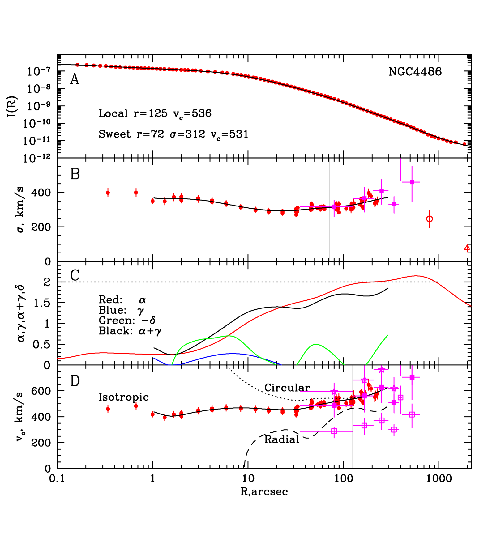
Figure 10: Circular speed in M87 estimated from the line-of-sight velocity dispersion using equations (25). Shown in panel A is the observed surface-brightness profile in the V band from Kormendy et al. (2009) ($I(R)=100^{-\mu/5}$, where $\mu$ is in magnitudes per arcsec²). Shown in panel B is the line-of-sight dispersion profile from Doherty et al. (2009). Black solid lines in panels A and B show smooth fitting curves. The magenta points with large error bars in panel B are the globular cluster data from Côté et al. (2001); these are shown for reference but are not used in any fits. The last two data points at 800-2000^′′ are the PNe data from Arnaboldi et al. (2004) (open circle) and Doherty et al. (2009) (open triangle). The fitting curves were used to compute $\alpha=-d\log I(R)/d\log R$, $\gamma=-d\log\sigma^{2}(R)/d\log R$, $\delta=d^{2}\log[I(R)\sigma^{2}]/d(\log R)^{2}$, and the sum $\alpha+\gamma$, which are shown in panel C by red, blue, green, and black lines. Shown in panel D are the estimated values of the circular speed. Red points in panel D correspond to the measured values of the line-of-sight velocity dispersion (shown in panel B), which were converted to the circular speed using equation (25) for isotropic orbits and the fitted curve for $\alpha+\gamma$ in panel C. The black solid, dotted and dashed curves are the result of applying equations (25) for isotropic, circular and radial orbits respectively to the smoothed curves approximating the surface brightness $I(R)$ and the line-of-sight dispersion $\sigma(R)$. The magenta points in panel D are the globular-cluster data converted to circular speed by approximating the surface density of globular clusters as a power law with $\alpha\approx 1.35$ and using equation (27) for circular (stars), isotropic (solid squares) and radial (open squares) models. Thin vertical lines in panels B and D show the radii used to estimate the circular speed using the methods, described in §3.2.1 and §3.3, respectively.

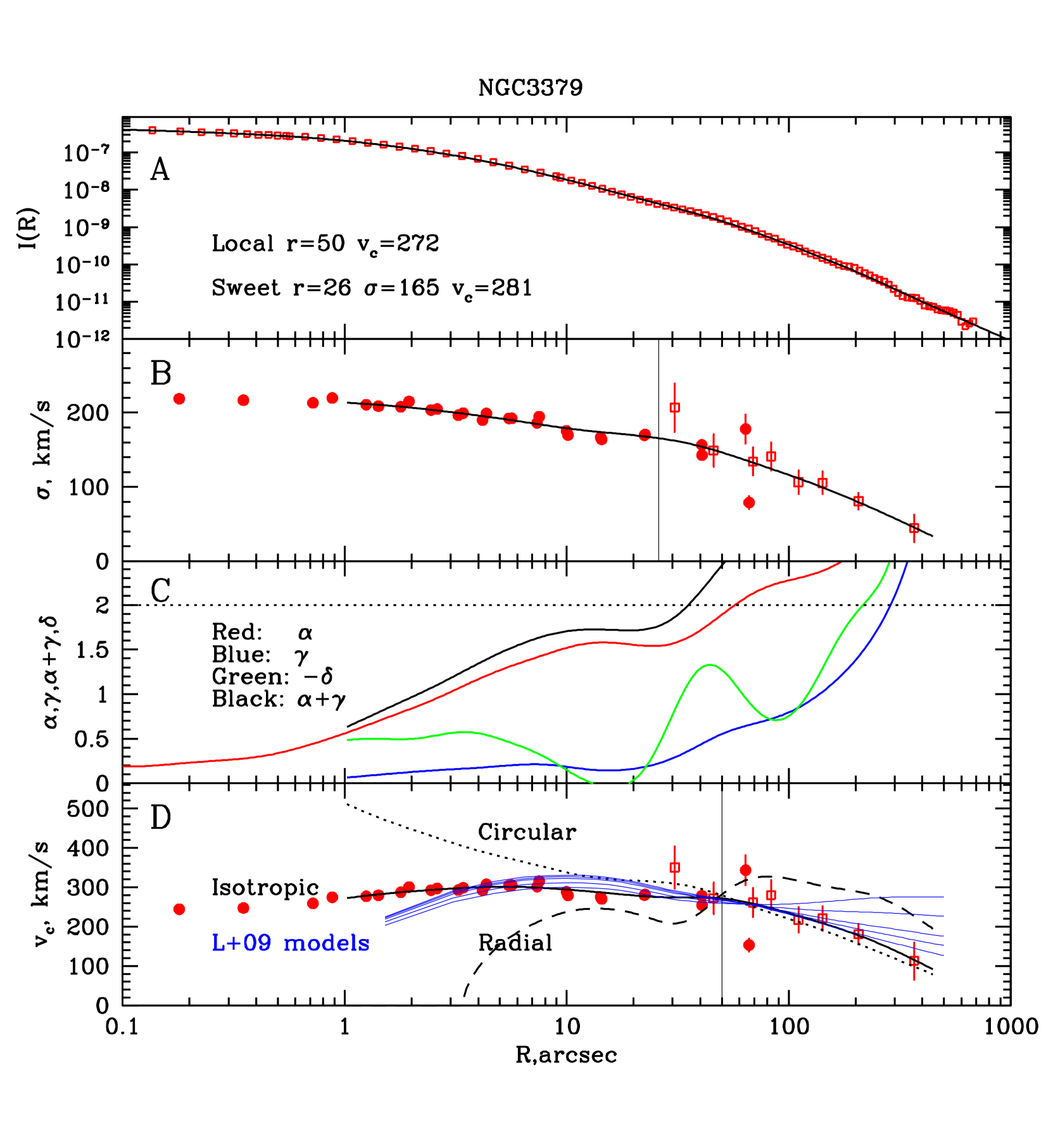
Figure 11: The same as in Figure 10 for NGC3379. Panel A shows the surface-brightness profile from wide-field B-band photometry by Capaccioli et al. (1990) and HST V-band observations from Gebhardt et al. (2000). The velocity dispersion (panel B) is from Statler & Smecker-Hane (1999) and Kronawitter et al. (2000), supplemented by planetary nebula velocity dispersions (points shown as open squares with large error bars at $R>30^{\prime\prime}$ in panel B, as calculated by de Lorenzi et al. 2009 from data in Douglas et al. 2007). Thin blue lines in panel D show the circular speeds from models A–E of de Lorenzi et al. (2009).

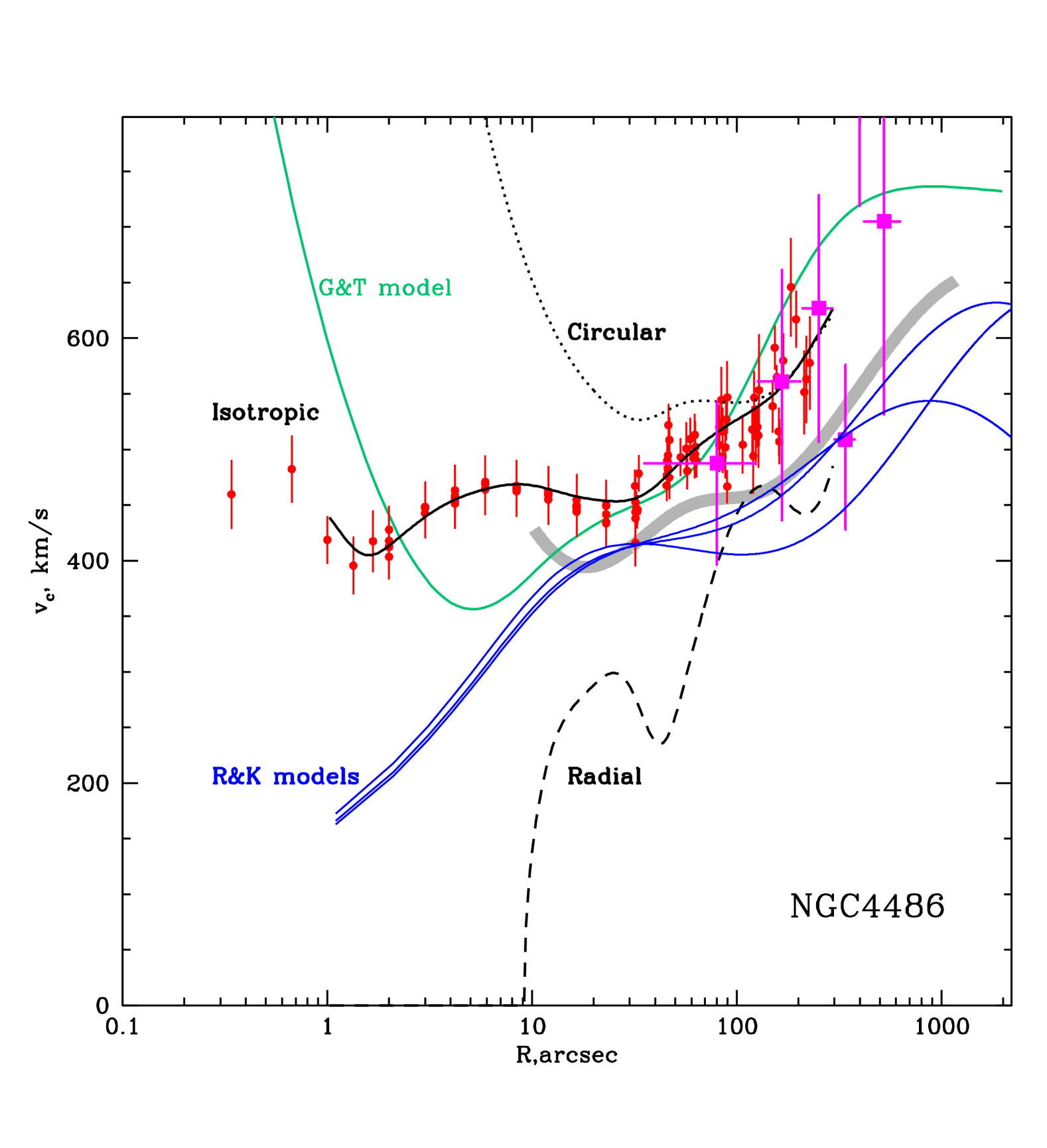
Figure 12: Circular speed in M87. Enlarged version of panel D of Figure 10. Blue lines show the circular speeds from the detailed dynamical analysis of Romanowsky & Kochanek (2001)—their models NFW1, NFW2, NFW3. The green line shows the best-fitting model of Gebhardt & Thomas (2009). The magenta points are the globular-cluster data converted to circular speed by approximating the surface density of globular clusters as a power law with $\alpha\approx 1.35$ and using equation (27) for isotropic systems. The thick gray curve is the circular speed derived from heavily smoothed X-ray data.

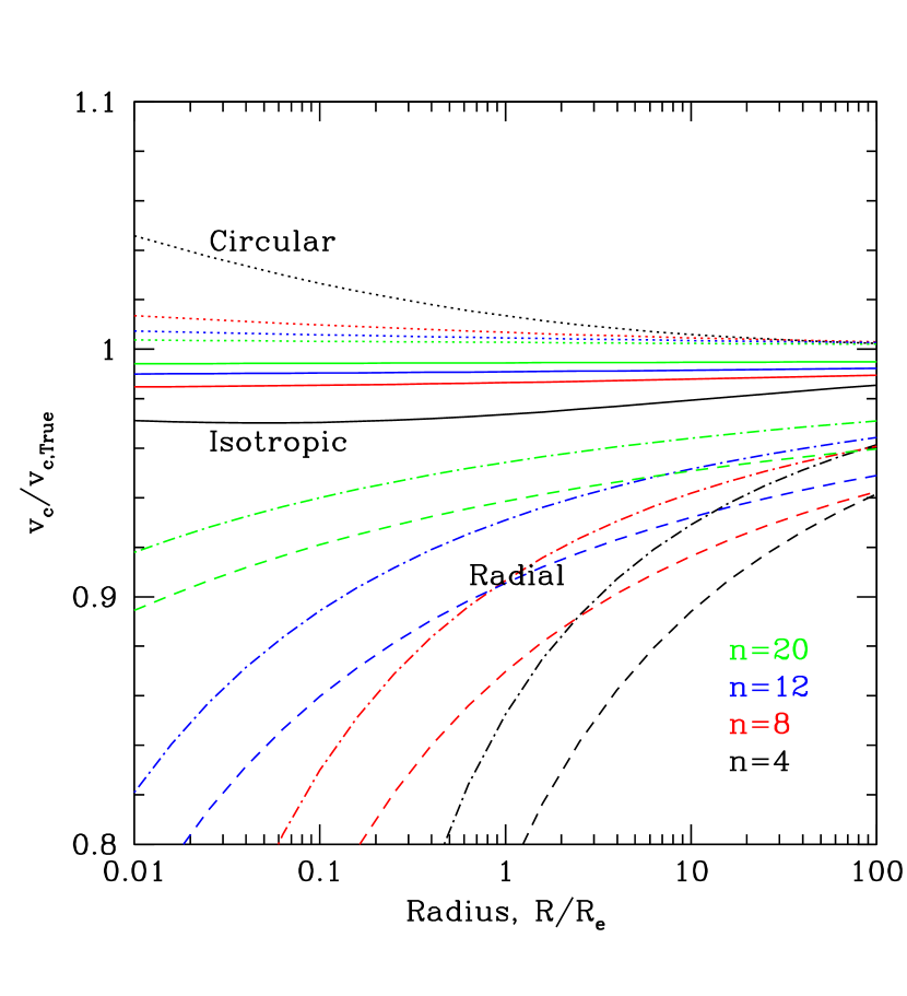
Figure 13: Circular speed estimated from the line-of-sight velocity dispersion using approximate equation (27) for isotropic (solid), circular (dotted) and radial (dashed) orbits, instead of the exact equation (25). The former equation uses a pure power law approximation to the surface brightness profile and completely ignores the terms $\gamma$ and $\delta$ (see §3.3). For radial orbits more accurate values of the circular speed are obtained (dash-dotted lines) from another approximate equation (28). Colors denote Sérsic models with $n=4,8,12$, and 20.

3.3.1 Circular speed varying with radius

Experiments in solving the Jeans equation for a galaxy with an $n=4$ Sérsic surface-brightness profile have shown that the local approximation works reasonably well at all radii even if the circular speed is not constant, provided that the orbital anisotropy is known and does not vary much with radius. This is illustrated in the left panel of Figure 14. Three types of model $v_{c}(r)$ profiles are shown in this figure with thick solid lines: (i) $v_{c}(r)={\rm const}$, (ii) $v_{c}(r)$ steadily rising with radius and (iii) $v_{c}(r)$ having a maximum at $r\sim R_{e}$ and declining towards smaller and larger radii. For each of the $v_{c}(r)$ profiles we calculated the projected velocity dispersion $\sigma(R)$, assuming constant anisotropy ($\beta=0,-9,1$) and converted $\sigma(R)$ back to $v_{c}(r)$ using eq. 25 for the appropriate type of anisotropy. The recovered $v_{c}(r)$ curves are shown in Figure 14 (left panel) with thin solid, dotted and dashed lines for isotropic, circular and radial orbits respectively. The vertical gray line shows the radius $R_{2}$ where $\displaystyle-d\log I(R)/d\log R=2$, which is close to the expected location of the region where the sensitivity of recovered $v_{c}(r)$ to the orbital anisotropy is smallest. Clearly the circular speed is recovered well even far away from $R_{2}$, if we can guess the anisotropy of the orbit distribution correctly.

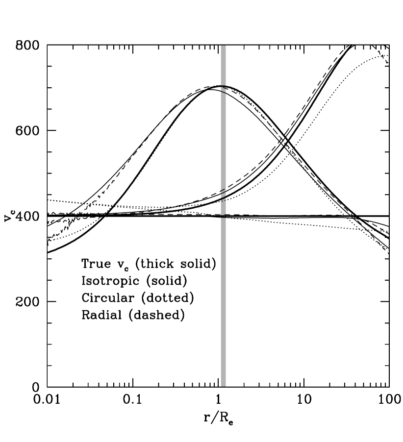
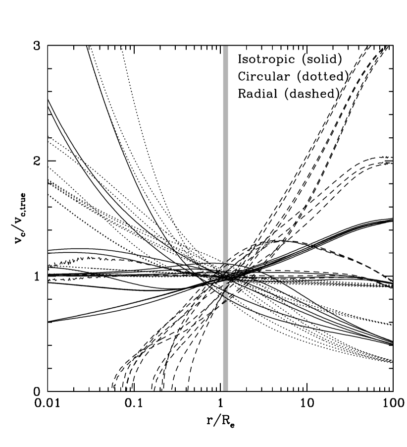
Figure 14: Left: Recovery of the non-constant circular speed profile from the the line-of-sight velocity dispersion profiles using eq. 25 when the anisotropy parameter is constant and known. Three types of model $v_{c}(r)$ profiles are shown with thick solid lines: (i) $v_{c}(r)={\rm const}$, (ii) $v_{c}(r)$ steadily rising with radius and (iii) $v_{c}(r)$ having a maximum at $r\sim R_{e}$ and declining towards smaller and larger radii. For each of the $v_{c}(r)$ profiles the line-of-sight velocity dispersion $\sigma(R)$ was calculated for $\beta=$ 0, -9, and 1 and converted back to $v_{c}(r)$ using eq. (25) for the isotropic (thin solid), circular (dotted) and radial (dashed) orbits. The vertical gray line shows the radius $R_{2}$ where $\displaystyle-\frac{d\log I(R)}{d\log R}=2$. The circular speed is recovered well even far away from $R_{2}$, if we know the anisotropy of orbit distribution. Right: Ratio of the recovered circular speed profile to the true circular speed profile when the true $v_{c}(r)$ is non-constant and the (unknown) anisotropy parameter varies with radius. The vertical gray line shows the radius $R_{2}$. Without prior knowledge of the orbital anisotropy the circular velocity profile can not be recovered accurately, except in the vicinity of $R_{2}$ where the spread in the $v_{c}$ values (including models with variable $v_{c}$ and $\beta$) is small.

If the anisotropy varies with radius the error introduced in the circular speed is similar in amplitude to that for the case of a logarithmic profile (Figure 6). Near the sweet point, defined according to equation (30), the value of $v_{c}$ is recovered to within $\sim$10-20% even if the circular speed is varying with radius. This is further illustrated in the right panel of Figure 14. In this figure we use the same three models of $v_{c}(r)$ profiles as in the left panel and five different models for the orbital anisotropy: the constant anisotropies $\beta=0,-9,1$, a model with orbits changing with radius from isotropic to radial ($c=1$, $\beta_{1}=0$, $\beta_{2}=1$, $r_{a}=2$ in eq. 21) and a model with orbits changing from isotropic to circular ($c=1$, $\beta_{1}=0$, $\beta_{2}=-9$, $r_{a}=2$ in eq. 21). For each combination of $v_{c}(r)$ and $\beta(r)$ we calculate the projected velocity dispersion $\sigma(R)$ and convert it back to the circular speed eq. 25 assuming constant anisotropy $\beta=0,-\infty,1$. This results in a total $3\times 5\times 3=45$ recovered circular speed profiles. The ratio of the recovered profiles to the true circular speed profiles is shown in Figure 14. Not surprisingly without any prior knowledge of the orbital anisotropy the circular speed profile can not be recovered accurately. However, in the vicinity of $R_{2}$ the spread in the $v_{c}$ values (including models with variable $v_{c}$ and $\beta$) is smallest: the ratio $\displaystyle v_{c}/v_{c,true}$ varies between 0.78 and 1.12 for the whole set of models.

At the radii where $\alpha$ is far from 2 (either smaller or larger) our method does not guarantee the recovery of $v_{c}$ without a firm prior on the anisotropy parameter. At these radii additional sources of information such as higher order velocity moments ($h_{3}$, $h_{4}$) and more elaborate methods (like Schwarzschild’s method) are needed. One example of a location where our method fails is the inner few arcsec in M87 where a black hole of a few times $10^{9}~{}M_{\odot}$ dominates the mass. Because the surface brightness is much flatter than $R^{-2}$ in this region the allowed range for the circular speed $v_{c}$ (for anisotropy $\beta$ between $-\infty$ and 1) is very wide (panel D of Fig. 10), easily large enough to accommodate a black hole with a mass ranging from 0 to $10^{10}~{}M_{\odot}$ or even larger.

3.4 Summary of suggested procedures for $v_{c}$ determination

3.4.1 For a galaxy with the surface-brightness profile well described by a Sérsic law

Use Table 4 (column 2) to find the “sweet spot radius” $R_{s}/R_{e}$ for a given $n$; use the line-of-sight velocity dispersion at this radius and convert it to the circular speed using column 3 of Table 4; we call this $v_{c,s}$ (see Table 1). Use column 4 from the same table to crudely estimate the uncertainty in $v_{c}$.

3.4.2 For a generic surface-brightness profile

Make a suitable interpolation of the surface-brightness profile (see, e.g., Appendix B) and the line-of-sight velocity dispersion profile. Calculate the slopes of these profiles (quantities $\alpha$, $\gamma$, $\delta$, as defined in §3.3). Convert interpolated line-of-sight velocity dispersion into circular speed using equations (25). Locate the sweet spot where the three curves are as close as possible (approximately corresponding to a range between radii where $\alpha\approx 2$ and $\alpha+\gamma\approx 2$) and use the circular speed value predicted by the curves in the vicinity of this radius. We call this $v_{c,l}$. When the curves do not intersect within the radial range well covered by the data (or in which, at least, the extrapolation is reasonable) one can use the radius where the range of circular speeds spanned by isotropic, circular and radial models is minimal. The difference between $v_{c}$ predicted by the three curves can be used to crudely characterize the uncertainty.

4 Results and discussion

Guided by the above considerations we compiled velocity dispersion measurements from the literature for the galaxy sample in Table 1.

• For the central velocity dispersion ($\sigma_{c}$) we rely on the Hyperleda database. The corresponding circular speed was estimated as $\displaystyle v_{c,c}=\sqrt{2}\sigma_{c}$, an approximation often used in the literature but with little or no theoretical justification (column 9 in Table 1).

• For the “sweet spot” estimates $R_{s}$ we use the values of the effective radius and the Sérsic index from Caon, Capaccioli, & D’Onofrio (1993), D’Onofrio, Capaccioli, & Caon (1994), Mahdavi, Trentham, & Tully (2005), and Spolaor et al. (2008). The values of $R_{s}$ were determined from the effective radius and Sérsic index using Table 4. The line-of-sight velocity dispersions at $R_{s}$ were taken from Kronawitter et al. (2000), Spolaor et al. (2008), Doherty et al. (2009) (and references therein), and De Bruyne et al. (2001). The corresponding values $\sigma(R_{s})$ are given in column 8 of the Table 1. In practice, for the selected sample $R_{s}$ is always close to 0.5$R_{e}$ and the ratio $\sigma_{iso}/v_{c}\simeq 0.6$. For one case when kinematic data do not extend to $R_{s}$ (NGC4472) we used the outermost data points to evaluate $\sigma$. Given the uncertainties in $R_{e}$, $n$ and the kinematics data, the accuracy of $\sigma$ is unlikely to be better than $\pm 5$–$10\,{\rm km~{}s}^{-1}$. In column 10 we estimate the circular speed using equation (14) for isotropic orbits (see also the entries for $\sigma_{\rm iso}$ in Table 4).

• For a second estimate of the circular speed we use the procedure described in §3.3: that is, we locate the region in which the logarithmic slopes $\alpha$ and $\alpha+\gamma$ (eqs. 26) are as close as possible to 2, find the line-of-sight dispersion $\sigma$ at this radius, and then estimate the circular speed using equation (25) for an isotropic model, as $\displaystyle v_{c,l}=\sigma\left(1+\alpha+\gamma\right)^{1/2}$. The values of $v_{c,l}$ for each galaxy in our sample are given in column 11 of Table 1. The most uncertain is the value of $v_{c,l}$ for NGC4472, where the kinematic data of Bender, Saglia, & Gerhard (1994) end at $R\simeq 40^{\prime\prime}$, while the Sérsic approximation to the surface brightness profile (Kormendy et al., 2009) suggests that the intersection of curves occurs at $\sim 200^{\prime\prime}$.

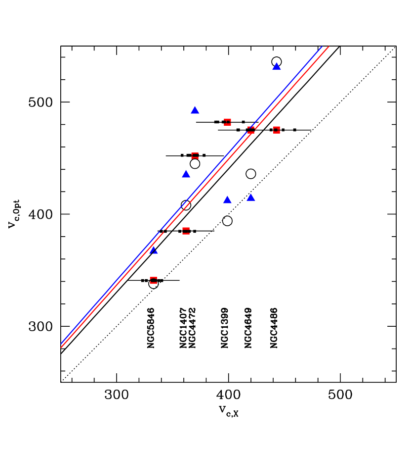
Figure 15: Relation between $v_{c,X}$, the estimate of the circular speed from X-ray data, and three forms of $v_{c,opt}$, the estimate from the optical data. Red squares - $v_{c,c}$, blue triangles - $v_{c,s}$, black circles - $v_{c,l}$. The dashed line corresponds to $v_{c,0pt}=v_{c,X}$, and solid red, blue and black lines to the best fitting relations between $v_{c,X}$ and $v_{c,c}$, $v_{c,s}$ and $v_{c,l}$ respectively. Small black squares shows the values of $v_{c,X}$ obtained when changes are made to the analysis procedure (see §2.4). These changes include: letting the abundance of heavy elements be a free parameter; adding a power law to account for potential contribution of LMXBs; varying lower or upper limits of the radial range used for $v_{c,X}$ calculations and separate calculations of the circular speed for the Northern and Southern parts of each galaxy. These different values of $v_{c,X}$ are plotted at fixed $v_{c,Opt}=v_{c,c}$ for each object. The black error bars show the crude estimate of the uncertainty in $v_{c,X}$ discussed in §2.4.

Following the discussion in §2 we compare the circular speed derived from the X-ray analysis (Table 2) with the three estimates of the circular speed from the optical data as shown in Figure 15. Assuming that $v_{c,opt}=\eta\times v_{c,X}$ we derive the following best fitting relations:

$$\begin{array}[]{lll}v_{c,c}&=1.12\times v_{c,X}&{\rm RMS}=0.07\\ v_{c,s}&=1.14\times v_{c,X}&{\rm RMS}=0.11\\ v_{c,l}&=1.10\times v_{c,X}&{\rm RMS}=0.09,\end{array}$$ (35)

where root-mean-square deviations were evaluated as ${\rm RMS}=\left[\sum_{i=1}^{N}\{v_{c,opt,i}/v_{c,X,i}-\eta\}^{2}/(N-1)\right]^{1/2}$, where summation is over the objects in the sample, $N=6$. We note here that the smallest scatter in the above relation is found for the circular speed estimated from the central velocity dispersion $v_{c,c}=\sqrt{2}\sigma_{c}$, rather than for more sophisticated estimates, which were constructed to be least sensitive to unknown orbit anisotropy. However, given the small size of our sample, no firm conclusion on the quality of different proxies to the circular speed is possible.

When five of the six objects are analyzed the value of $\eta$ varies from 1.07 to 1.13 for $v_{c,l}$ (compared to 1.10 for the full sample of six objects). The conclusion that $\eta>1$ continues to holds. One can also estimate the significance of the statement that $\eta>1$ from the fact that almost all of the points are in Figure 15 are in the upper left part of the plot. Assuming that $\eta$ can equally probably be larger or smaller than unity the probability that 6 out of 6 points (for $v_{c,c}$) or 5 out of 6 (for $v_{c,s}$ and $v_{c,l}$) are found with $\eta>1$ is 0.016 and 0.11 respectively.

As discussed in §2.4 changing the assumptions made in the analysis of X-ray data affects the value of $v_{c,X}$. This includes the effect of variable metalicity, contribution of LMXBs, dependence on the radial range used for evaluation of $v_{c,X}$ and independent calculations of the circular speed for the Northern and Southern parts of each galaxy. The values of $v_{c,X}$ obtained in each of the tests described in §2.4 are shown with small black squares in Figure 15. For clarity these values of $v_{c,X}$ are plotted at the same $v_{c,Opt}=v_{c,c}$. The black error bars show the crude estimate of the uncertainty in $v_{c,X}$ of $\sim$7% obtained in §2.4 under simplifying assumption that the contributions of different effects co-add quadratically.

As discussed in C08 the derived value of $v_{c,X}$ is sensitive to non-thermal forms of pressure support. This non-thermal support can be parametrized by its impact on the relation between $v_{c,X}$ and the true circular speed $v_{c}$:

$$v^{2}_{c}=v^{2}_{c,X}\left(1+\frac{P_{n}}{P_{g}}\right),$$ (36)

where $P_{n}$ and $P_{g}$ are the non-thermal and gas thermal pressures respectively. Thus the observed relation (eq. 35) provides a measure of $P_{n}/P_{g}$:

$$\frac{P_{n}}{P_{g}}\approx\eta^{2}-1\approx 0.21-0.29,$$ (37)

depending on the adopted estimator of the optical velocity dispersion in equation (35).

There are a number of obvious caveats (both on the X-ray and the optical sides) associated with the above analysis. In particular there is considerable uncertainty in the heavy metal abundance determination, mentioned in §2, which may affect the estimates of the potential at the level of a few per cent. Some of our galaxies sit in massive group/cluster halos; in such cases the circular speed increases at large radii (e.g. M87 - see Figure 12), so the approximation of the potential as a logarithmic law characterized by a single circular speed may not be sufficient for accurate comparison of the X-ray and optical data over several decades of radius. Minor deviations from hydrostatic equilibrium, visible as wiggles in the potential profiles, could also contribute to the scatter. Nevertheless we believe that our main result—that the depth of the potential well derived from X-ray data (from hot gas) is systematically shallower (by few tens of percents) than the corresponding optical value (from stars)—is robust. As mentioned in C08 these values are consistent with the current paradigm of AGN controlled gas cooling/heating in the centers of clusters and individual massive elliptical galaxies (e.g., Churazov et al., 2002). The key assumptions of this paradigm are that:

• Gas radiative cooling losses are balanced by the mechanical energy provided by a central black hole (AGN);

• Dissipation of the mechanical energy is occurring on time scales comparable (within a factor of few) to the sound crossing time of the cooling region;

• The ratio of the dissipation and cooling time scales (of the order of 0.1–0.2) sets the ratio of the non-thermal and thermal energy densities.

We finally note that the sample considered here is not statistically complete and generalization of these results to all gas-rich ellipticals must be done with caution.

5 Conclusions

Using non-parametric method we reconstructed gravitating potentials for a sample of six X-ray bright elliptical galaxies observed with Chandra and XMM-Newton. Their gravitational potentials can be reasonably well approximated by the isothermal (logarithmic) law $v_{c,X}\log r+b$ over the range of radii from $\sim$0.5 to $\sim$25 kpc, corresponding to $\sim 0.05$–$3~{}R_{e}$. This result is in line with recent lensing data which also suggest isothermality of the gravitational potentials of the early-type galaxies and earlier results based on stellar kinematics and X-ray data. Many galaxies in our sample are located at centers of massive groups/clusters and the X-ray data going beyond the optical extent of galaxies show the steepening of the potential at large radii.

We suggest two new methods to derive an estimate of a galaxy’s circular speed if its potential is described by the isothermal law. (i) For a spherical galaxy with a given Sérsic index $n$, the line-of-sight stellar velocity dispersion $\sigma_{opt}(R_{s})$ evaluated at $R_{s}=R_{s}(n)\approx 0.5R_{e}$ turns out to be relatively insensitive to the anisotropy of stellar orbits. (ii) We suggest the extension of this method for a generic surface-brightness profile which allows one to estimate the circular speed through the “local” values of the line-of-sight velocity dispersion and the logarithmic derivatives of the surface brightness and the velocity-dispersion profiles.

Application of these methods to a sample of six massive elliptical galaxies and the comparison to the results of X-ray analysis suggests that on average 20% of the gas pressure in these galaxies is provided by non-thermal components (e.g., micro-turbulence or cosmic rays). This result is in broad agreement with the current paradigm of AGN controlled gas cooling/heating in the centers of clusters and individual massive elliptical galaxies.

6 Acknowledgments

We are grateful to Guinevere Kauffmann, Ben Metcalf, and Glenn van de Ven for useful discussions. This work was supported by the DFG grant CH389/3-2; NASA contracts and grants NAS8-38248, NAS8-01130, NAS8-03060, and NNX08AH24G; the program “Extended objects in the Universe” of the Division of Physical Sciences of the RAS; the Chandra Science Center; the Smithsonian Institution; MPI für Astrophysik; MPI für Extraterrestrische Physik and the Cluster of Excellence “Origin and Structure of the Universe”. ST acknowledges support from a Humboldt Research Award.

Appendix A Line-of-sight velocity dispersion in a logarithmic potential

The goal of this Appendix is to derive formulae for the line-of-sight velocity dispersion profile $\sigma(R)$ for a spherical galaxy with surface-brightness profile $I(R)$, assuming that the gravitational potential is logarithmic,

$$\phi(r)=v_{c}^{2}\log r+\hbox{const}.$$ (38)

The line-of-sight dispersion will depend on the shape of the velocity-dispersion tensor, defined by its radial and tangential components $\sigma_{r}^{2}(r)$ and $\sigma_{\phi}^{2}(r)=\sigma_{\theta}^{2}(r)$. We examine three simple cases that should span the range of possible behaviors: (i) isotropic orbits ($\sigma_{r}^{2}=\sigma_{\phi}^{2}=\sigma_{\theta}^{2}$); (ii) radial orbits ($\sigma_{\phi}^{2}=\sigma_{\theta}^{2}=0$); (iii) circular orbits ($\sigma_{r}^{2}=0$).

In a spherical system, the volume emissivity $j(r)$ and the surface brightness $I(R)$ are related by

$$I(R) = 2\int_{R}^{\infty}\!\!{r\,dr\over\sqrt{r^{2}-R^{2}}}j(r),$$

$$j(r) = -{1\over\pi}\int_{r}^{\infty}\!\!{dR\over\sqrt{R^{2}-r^{2}}}{dI\over dR}.$$ (39)

If the system is isotropic, the Jeans equation reads

$${d\over dr}j\sigma_{r}^{2}=-j{d\phi\over dr}.$$ (40)

Specializing to the logarithmic potential and integrating

$$j(r)\sigma_{r}^{2}(r)=v_{c}^{2}\int_{r}^{\infty}{du\over u}j(u).$$ (41)

The line-of-sight dispersion at projected radius $R$, $\sigma_{\rm iso}(R)$, is given by

$$I(R)\sigma_{\rm iso}^{2}(R) = 2\int_{R}^{\infty}{r\,dr\over\sqrt{r^{2}-R^{2}}}j(r)\sigma_{r}^{2}(r)$$ (42)

$$= 2v_{c}^{2}\int_{R}^{\infty}{r\,dr\over\sqrt{r^{2}-R^{2}}}\int_{r}^{\infty}{du\over u}j(u)$$

$$= 2v_{c}^{2}\int_{R}^{\infty}{du\sqrt{u^{2}-R^{2}}\over u}j(u).$$

Replacing $j(u)$ from equation (39) and exchanging the order of integration,

$$I(R)\sigma_{\rm iso}^{2}(R)=-{2v_{c}^{2}\over\pi}\int_{R}^{\infty}dx{dI\over dx}\int_{R}^{x}{\sqrt{u^{2}-R^{2}}\,du\over u\sqrt{x^{2}-u^{2}}}.$$ (43)

The inner integral is ${\textstyle{1\over 2}}\pi(1-R/x)$ so after integrating by parts

$$I(R)\sigma_{\rm iso}^{2}(R)=Rv_{c}^{2}\int_{R}^{\infty}\frac{I(x)}{x^{2}}dx,$$ (44)

which is equation (14).

If the orbits are circular, a set of stars with random orientation at radius $r$ and projected radius $R$ contributes a line-of-sight dispersion ${\textstyle{1\over 2}}v_{c}^{2}R^{2}/r^{2}$. Thus the line-of-sight dispersion at $R$ is given by

$$I(R)\sigma_{\rm circ}^{2}(R)=R^{2}v_{c}^{2}\int_{R}^{\infty}{dr\over r\sqrt{r^{2}-R^{2}}}j(r).$$ (45)

Replacing $j(r)$ from equation (39) and exchanging the order of integration,

$$I(R)\sigma_{\rm circ}^{2}(R) = -{R^{2}v_{c}^{2}\over\pi}\int_{R}^{\infty}dx{dI\over dx}$$ (46)

$$\quad\times\int_{R}^{x}{dr\over r\sqrt{r^{2}-R^{2}}\sqrt{x^{2}-r^{2}}}.$$

The inner integral is ${\textstyle{1\over 2}}\pi/(Rx)$ so after integrating by parts

$$\sigma_{\rm circ}^{2}(R) = {\textstyle{1\over 2}}v_{c}^{2}-{Rv_{c}^{2}\over 2I(R)}\int_{R}^{\infty}\frac{I(x)}{x^{2}}dx$$ (47)

$$= {\textstyle{1\over 2}}v_{c}^{2}-{\textstyle{1\over 2}}\sigma_{\rm iso}^{2}(R),$$

which is equation (15).

Finally, if the orbits are radial, the Jeans equation reads

$${d\over dr}r^{2}j\sigma_{r}^{2}=-jr^{2}{d\phi\over dr}.$$ (48)

Specializing to the logarithmic potential and integrating,

$$j(r)\sigma_{r}^{2}(r)={v_{c}^{2}\over r^{2}}\int_{r}^{\infty}du\,uj(u).$$ (49)

If the orbits are radial, a set of stars at radius $r$ and projected radius $R$ contributes a line-of-sight dispersion $\sigma_{r}^{2}(r)(r^{2}-R^{2})/r^{2}$. The line-of-sight dispersion at projected radius $R$, $\sigma_{\rm rad}(R)$, is then given by

$$I(R)\sigma_{\rm rad}^{2}(R) = 2\int_{R}^{\infty}{dr\sqrt{r^{2}-R^{2}}\over r}j(r)\sigma_{r}^{2}(r)$$ (50)

$$= 2v_{c}^{2}\int_{R}^{\infty}{dr\sqrt{r^{2}-R^{2}}\over r^{3}}\int_{r}^{\infty}du\,uj(u).$$

Replacing $j(u)$ from equation (39) and exchanging the order of integration,

$$I(R)\sigma_{\rm rad}^{2}(R) = -{2v_{c}^{2}\over\pi}\int_{R}^{\infty}{dr\sqrt{r^{2}-R^{2}}\over r^{3}}\int_{r}^{\infty}dx\sqrt{x^{2}-r^{2}}{dI\over dx}$$ (51)

$$= {2v_{c}^{2}\over\pi}\int_{R}^{\infty}{dr\sqrt{r^{2}-R^{2}}\over r^{3}}\int_{r}^{\infty}{x\,dx\over\sqrt{x^{2}-r^{2}}}I(x)$$

$$= {2v_{c}^{2}\over\pi}\int_{R}^{\infty}dx\,xI(x)\int_{R}^{x}{dr\over r^{3}}{\sqrt{r^{2}-R^{2}}\over\sqrt{x^{2}-r^{2}}}.$$

The inner integral is ${1\over 4}\pi(x^{2}-R^{2})/(Rx^{3})$, so

$$I(R)\sigma_{\rm rad}^{2}(R)={v_{c}^{2}\over 2R}\int_{R}^{\infty}I(x)(1-R^{2}/x^{2})dx,$$ (52)

which is equation (16).

Appendix B Smoothing the surface-brightness profile

The procedure for evaluating the circular speed that is described in §3.3 requires calculations of the derivatives of the surface brightness $I(R)$ and the line-of-sight velocity dispersion $\sigma(R)$. The derivative of the surface brightness is expected to be the most important term (see Fig. 8). The observed surface-brightness profiles typically have enough data points with small errorbars to make the selection of a simple analytic model difficult. To counter this problem we used a simple procedure to smooth the data. Consider a set of surface brightness measurements $I(R_{i}),i=1,\ldots,n$. Given that we are interested primarily in logarithmic derivatives it makes sense to use $f_{i}=\log R_{i}$ and $S_{i}=\log I(R_{i})$ instead of $R$ and $I$. We can then fit the linear relation between $f_{i}$ and $S_{i}$ as $S_{i}=af_{i}+b$, where $a$ and $b$ are the free parameters of the fit. We want to find “local” values of $a$ and $b$ in the vicinity of a given radius $R_{0}$, which are based on a set of measurements not far from $R_{0}$. We do that by choosing a weight function

$$W(R_{0},R)=\exp\left[-\frac{(\log R_{0}-\log R)^{2}}{2\Delta^{2}_{R}}\right],$$ (53)

where the parameter $\Delta_{R}$ controls the width of the weight function. The best fitting parameters $a$ and $b$ (minimizing RMS deviation) for a given value of $f_{0}\equiv\log R_{0}$ are given by

$$a(R_{0})=\frac{\sum f_{i}W_{i}S_{i}\sum W_{i}-\sum W_{i}S_{i}\sum f_{i}W_{i}}{\sum f^{2}_{i}W_{i}\sum W_{i}-(\sum_{i}f_{i}W_{i})^{2}},$$ (54)

where $W_{i}=W(R_{0},R_{i})$, the sums are over $i=1,\ldots,n$, and

$$b(R_{0})=\frac{\sum_{i}W_{i}S_{i}-a\sum_{i}f_{i}W_{i}}{\sum_{i}W_{i}}.$$ (55)

The smoothed function $\tilde{I}(R)=e^{a(R)\log R+b(R)}$ is shown in panel A in Figures 10 and 11 with a black solid line. We used $\Delta_{R}=0.3$ for both objects.

References

- Anders & Grevesse (1989) Anders E., Grevesse N. 1989, Geochim. Cosmochim. Acta, 53, 197
- Arnaboldi et al. (2004) Arnaboldi M., Gerhard O., Aguerri J.A.L., Freeman K.C., Napolitano N.R., Okamura S., Yasuda N. 2004, ApJ, 614, L33
- Arnaud (1996) Arnaud, K.A. 1996, Astronomical Data Analysis Software and Systems V, 101, 17
- Bender, Saglia, & Gerhard (1994) Bender R., Saglia R.P., Gerhard O.E. 1994, MNRAS, 269, 785
- Buote & Canizares (1994) Buote D.A., Canizares C.R. 1994, ApJ, 427, 86
- Buote & Canizares (1998) Buote D.A., Canizares C.R. 1998, MNRAS, 298, 811
- Buote (2000) Buote D.A. 2000, ApJ, 539, 172
- Caon, Capaccioli, & D’Onofrio (1993) Caon N., Capaccioli M., D’Onofrio M. 1993, MNRAS, 265, 1013
- Capaccioli et al. (1990) Capaccioli M., Held E.V., Lorenz H., Vietri M. 1990, AJ, 99, 1813
- Cappellari et al. (2006) Cappellari M., et al. 2006, MNRAS, 366, 1126
- Castro-Rodríiguez et al. (2003) Castro-Rodríguez, N., et al. 2003, A&A, 405, 803
- Churazov et al. (2002) Churazov E., Sunyaev R., Forman W., Böhringer H. 2002, MNRAS, 332, 729
- Churazov et al. (2003) Churazov E., Forman W., Jones C., Böhringer H. 2003, ApJ, 590, 225
- Churazov et al. (2008) Churazov E., Forman W., Vikhlinin A., Tremaine S., Gerhard O., Jones C. 2008, MNRAS, 388, 1062
- Chuzhoy & Nusser (2003) Chuzhoy L., Nusser A. 2003, MNRAS, 342, L5
- Chuzhoy & Loeb (2004) Chuzhoy L., Loeb A. 2004, MNRAS, 349, L13
- Coccato et al. (2009) Coccato L., et al. 2009, MNRAS, 394, 1249
- Côté et al. (2001) Côté P., et al. 2001, ApJ, 559, 828
- David et al. (2006) David L.P., Jones C., Forman W., Vargas I.M., Nulsen P. 2006, ApJ, 653, 207
- De Bruyne et al. (2001) De Bruyne V., Dejonghe H., Pizzella A., Bernardi M., Zeilinger W.W. 2001, ApJ, 546, 903
- de Lorenzi et al. (2009) de Lorenzi F., et al. 2009, MNRAS, 395, 76
- Doherty et al. (2009) Doherty M., et al. 2009, A&A, in press
- D’Onofrio, Capaccioli, & Caon (1994) D’Onofrio M., Capaccioli M., Caon N. 1994, MNRAS, 271, 523
- Douglas et al. (2007) Douglas N.G., et al. 2007, ApJ, 664, 257
- Emsellem et al. (2004) Emsellem E., et al., 2004, MNRAS, 352, 721
- Ettori & Fabian (2006) Ettori S., Fabian A.C. 2006, MNRAS, 369, L42
- Fabian et al. (1981) Fabian A. C., Hu E. M., Cowie L. L., Grindlay J., 1981, ApJ, 248, 47
- Forman, Jones, & Tucker (1985) Forman W., Jones C., Tucker W. 1985, ApJ, 293, 102
- Fukazawa et al. (2006) Fukazawa Y., Botoya-Nonesa J.G., Pu J., Ohto A., Kawano N. 2006, ApJ, 636, 698
- Gavazzi et al. (2007) Gavazzi R., Treu T., Rhodes J.D., Koopmans L.V.E., Bolton A.S., Burles S., Massey R.J., Moustakas L.A., 2007, ApJ, 667, 176
- Gebhardt et al. (2000) Gebhardt K., et al. 2000, AJ, 119, 1157
- Gebhardt & Thomas (2009) Gebhardt K., Thomas J., 2009, ApJ, 700, 1690
- Murhphy & Gebhardt (2009) Gebhardt K., 2009, to be submitted
- Gerhard (1993) Gerhard O.E. 1993, MNRAS, 265, 213
- Gerhard et al. (2001) Gerhard O., Kronawitter A., Saglia R.P., Bender R. 2001, AJ, 121 1936
- Gilfanov & Sunyaev (1984) Gilfanov M.R., Sunyaev R.A. 1984, SvAL, 10, 137
- Graham & Driver (2005) Graham A.W., Driver S.P. 2005, Publications of the Astronomical Society of Australia, 22, 118
- Gültekin et al. (2009) Gültekin K., et al. 2009, ApJ, 695, 1577
- Hill et al. (2008) Hill G. J., et al., 2008, SPIE, 7014
- Humphrey et al. (2006) Humphrey P., Buote D., Gastaldello F., Zappacosta L., Bullock J., Brighenti F., Mathews W. 2006, ApJ, 646, 899
- Humphrey & Buote (2006) Humphrey P.J., Buote D.A., 2006, ApJ, 639, 136
- Humphrey et al. (2008) Humphrey P. J., Buote D. A., Brighenti F., Gebhardt K., Mathews W. G., 2008, ApJ, 683, 161
- Irwin, Athey, & Bregman (2003) Irwin J.A., Athey A.E., Bregman J.N. 2003, ApJ, 587, 356
- Kalberla et al. (2005) Kalberla P.M.W., Burton W.B., Hartmann D., Arnal E.M., Bajaja E., Morras R., Pöppel W.G.L. 2005, A&A, 440, 775
- Kim & Fabbiano (1995) Kim D.-W., Fabbiano G. 1995, ApJ, 441, 182
- Klypin & Prada (2009) Klypin A., Prada F. 2009, ApJ, 690, 1488
- Koopmans et al. (2006) Koopmans L. V. E., Treu T., Bolton A. S., Burles S., Moustakas L. A., 2006, ApJ, 649, 599
- Kormendy et al. (2009) Kormendy J., Fisher D.B., Cornell M.E., Bender R. 2009, ApJS, 182, 216
- Kronawitter et al. (2000) Kronawitter A., Saglia R.P., Gerhard O., Bender R. 2000, A&AS, 144, 53
- Mahdavi, Trentham, & Tully (2005) Mahdavi A., Trentham N., Tully R.B. 2005, AJ, 130, 1502
- Mandelbaum et al. (2006) Mandelbaum R., Seljak U., Kauffmann G., Hirata C.M., Brinkmann J. 2006, MNRAS, 368, 715
- Mandelbaum, van de Ven, & Keeton (2008) Mandelbaum R., van de Ven G., Keeton C.R. 2008, arXiv:0808.2497
- Mathews (1978) Mathews W. 1978, ApJ, 219, 413
- Matsushita et al. (2002) Matsushita K., Belsole E., Finoguenov A., Böhringer H., 2002, A&A, 386, 77
- Merritt (1985) Merritt D. 1985, AJ, 90, 1027
- Nulsen & Bohringer (1995) Nulsen P. E. J., Bohringer H., 1995, MNRAS, 274, 1093
- Osipkov (1979) Osipkov L.P. 1979, SvAL, 5, 42
- Padmanabhan et al. (2004) Padmanabhan N., et al., 2004, NewA, 9, 329
- Piffaretti, Jetzer, & Schindler (2003) Piffaretti R., Jetzer P., Schindler S., 2003, A&A, 398, 41
- Revnivtsev et al. (2008) Revnivtsev M., Churazov E., Sazonov S., Forman W., Jones C. 2008, A&A, 490, 37
- Richstone & Tremaine (1984) Richstone D.O., Tremaine S. 1984, ApJ, 286, 27
- Romanowsky & Kochanek (2001) Romanowsky A.J., Kochanek C.S. 2001, ApJ, 553, 722
- Saglia et al. (2000) Saglia R. P., Kronawitter, A., Gerhard O., Bender, R. 2000, AJ, 119,153
- Smith et al. (2001) Smith R.K., Brickhouse N.S., Liedahl D.A., Raymond J.C. 2001, ApJ, 556, L91
- Spolaor et al. (2008) Spolaor M., Forbes D.A., Hau G.K.T., Proctor R.N., Brough S. 2008, MNRAS, 385, 667
- Statler & Smecker-Hane (1999) Statler T.S., Smecker-Hane T. 1999, AJ, 117, 839
- Thomas et al. (2007) Thomas J., Saglia R.P., Bender R., Thomas D., Gebhardt K., Magorrian J., Corsini E.M., Wegner G., 2007, MNRAS, 382, 657
- Tonry et al. (2001) Tonry J. L., Dressler A., Blakeslee J. P., Ajhar E. A., Fletcher A. B., Luppino G. A., Metzger M. R., Moore C. B., 2001, ApJ, 546, 681
- Treu et al. (2006) Treu T., Koopmans L.V., Bolton A.S., Burles S., Moustakas L.A. 2006, ApJ, 640, 662
- Trinchieri & Fabbiano (1985) Trinchieri G., Fabbiano G. 1985, ApJ, 296, 447
- van der Marel (1994) van der Marel R. P., 1994, MNRAS, 270, 271
- Vikhlinin et al. (2005) Vikhlinin A., Markevitch M., Murray S.S., Jones C., Forman W., Van Speybroeck L. 2005, ApJ, 628, 655