The $\ell_{1}$-norm in quantum information via the approach of Yang-Baxter Equation

Abstract

The role of $\ell_{1}$-norm in Quantum Mechanics (QM) has been studied through Wigner’s D-functions where $\ell_{1}$-norm means $\sum_{i}\left|C_{i}\right|$ for $\left|\Psi\right\rangle=\sum_{i}C_{i}\left|\psi_{i}\right\rangle$ if $\left|\psi_{i}\right\rangle$ are uni-orthogonal and normalized basis. It was shown that the present two types of transformation matrix acting on the natural basis in physics consist in an unified braiding matrix, which can be viewed as a particular solution of the Yang-Baxter equation (YBE). The maximum of the $\ell_{1}$-norm is connected with the maximally entangled states and topological quantum field theory (TQFT) with two-component anyons while the minimum leads to the permutation for fermions or bosons.

I Introduction: two types of braiding matrices, Yang-Baxter equation and Temperley-Lieb algebra

The purpose of this paper is committed to clarifying how $\ell_{1}$-norm participates in Quantum Mechanics (QM) and demonstrating the physical meaning through acceptable physical examples. In QM, a wave function $\left|\Psi\right\rangle$ can be decomposed to $\left|\Psi\right\rangle=\sum_{i}C_{i}\left|\psi_{i}\right\rangle$, where $\left|\psi_{i}\right\rangle$ is uni-orthogonal basis and the normalizability of $\left|\Psi\right\rangle$ reads

$$\langle\Psi\left|\Psi\right\rangle =\sum_{i}\left|C_{i}\right|^{2}=1.$$ (1)

We call $\sum_{i}\left|C_{i}\right|^{2}=\left\|C\right\|_{\ell_{2}}$ as $\ell_{2}$-norm, which indicates the square integrability of the wave function. Meanwhile the notation $\sum_{i}\left|C_{i}\right|=\left\|C\right\|_{\ell_{1}}$ is called $\ell_{1}$-norm.

We may ask whether an $\ell_{1}$-norm $f=\sum_{i}\left|C_{i}\right|$ plays role in QM and if so, which physical model represents this statement. For this target, we should go a long way. We shall show that the local maximum and minimum of $\ell_{1}$-norm will lead to two types of braiding matrices that have existed in physics. One is related to the entangled states including the anyonic description 1 ; 2 ; 3 , and the other to the permutation type 4 , which lays down the base of solvable models exactly 4 ; 5 . In order to explain the matter clearly, we have to begin with the braid relation, Yang-Baxter Equation (YBE), and their particular matrix forms. And then the physical consequence of extremism of $\ell_{1}$-norm was explained.

Recently, a new development has been used to connect the braid matrix, as well as the YBE, with the entangled states 6 ; 7 ; 8 ; 9 ; 10 ; 11 . We start the discussion with the maximally entangled states, i.e., the Bell states. For a two-qubit system, Bell states are defined by:

$$\left|\Phi^{\pm}\right\rangle =\frac{1}{\sqrt{2}}\left(\left|\uparrow\uparrow\right\rangle\pm\left|\downarrow\downarrow\right\rangle\right),$$

$$\left|\Psi^{\pm}\right\rangle =\frac{1}{\sqrt{2}}\left(\left|\uparrow\downarrow\right\rangle\pm\left|\downarrow\uparrow\right\rangle\right).$$

The Bell states are connected to the natural basis $\left|\psi_{0}\right\rangle=(\left|\uparrow\uparrow\right\rangle,\left|\uparrow\downarrow\right\rangle,\left|\downarrow\uparrow\right\rangle,\left|\downarrow\downarrow\right\rangle)^{T}$ by a unitary transformation matrix $W$, which satisfies

$$\left(\Phi^{+},\Psi^{+},-\Psi^{-},-\Phi^{-}\right) =W\left(\left|\uparrow\uparrow\right\rangle,\left|\uparrow\downarrow\right\rangle,\left|\downarrow\uparrow\right\rangle,\left|\downarrow\downarrow\right\rangle\right)^{T},$$ (2)

where

$$W =\frac{1}{\sqrt{2}}\left(\begin{array}[]{cccc}1&0&0&1\\ 0&1&1&0\\ 0&-1&1&0\\ -1&0&0&1\end{array}\right).$$

The $W$ can be extended to matrix $b$ such as 7 ; 10

$$b_{\mbox{I}}(q) =\frac{1}{\sqrt{2}}\left(\begin{array}[]{cccc}1&0&0&q\\ 0&1&\epsilon&0\\ 0&-\epsilon&1&0\\ -q^{-1}&0&0&1\end{array}\right)=\frac{1}{\sqrt{2}}(1+M),$$ (7)

$$\epsilon^{2} =1,\quad M^{2}=-1,\quad q=e^{i\alpha}.$$ (8)

Kauffman et al. 7 have shown that the matrix $W$ is nothing but a braid matrix ($N^{2}=4$), which satisfies

$$B_{1}B_{2}B_{1} =B_{2}B_{1}B_{2},$$ (9)

where

$$B_{1}^{\mbox{I}} \equiv B_{12}^{\mbox{I}}=b_{\mbox{I}}(q)\otimes I,$$

$$B_{2}^{\mbox{I}} \equiv B_{23}^{\mbox{I}}=I\otimes b_{\mbox{I}}(q).$$

On the other hand, in solving a one-dimensional (1D) model with $\delta$-function potential 12 , and a low-dimensional statistical model, as well as the chain models, the other types of braiding matrices were introduced years ago13 . The simplest form is given by 14

$$b_{\mbox{II}}=\left(\begin{array}[]{cccc}q&0&0&0\\ 0&0&-\eta&0\\ 0&-\eta^{-1}&q-q^{-1}&0\\ 0&0&0&q\end{array}\right),$$ (14)

that was known as the $q$-deformation of permutation. Here $\eta=e^{i\alpha}$ with $\alpha$ being any flux, when $\eta=-1$, $q=1$, Eq. (14) reduces to the permutation, which is universal symmetry operator for identical particles either boson or fermion. A braiding matrix can be viewed as the asymptotic behavior of $2$-body scattering matrix, i.e., the momenta independent part of S-matrix. For a given matrix satisfying Eq. (9), the corresponding $\breve{R}(x)$-matrix can obey

$$\breve{R}_{1}(x)\breve{R}_{2}(xy)\breve{R}_{1}(y) =\breve{R}_{2}(y)\breve{R}_{1}(xy)\breve{R}_{2}(x),$$ (15)

where $x$ is spectral parameter related to 1D momenta($u$ for $x=e^{iu}$) which obeys the conservation law, and

$$\breve{R}_{1}(x)\equiv\breve{R}_{12}(x) =\breve{R}(x)\otimes I,$$

$$\breve{R}_{2}(x)\equiv\breve{R}_{23}(x) =I\otimes\breve{R}(x).$$

Obviously, matrix $B$ is a particular case of $\breve{R}(x)$. The physical meaning of $\breve{R}(x)$ is the S-matrix of $2$-body scattering. Eq. (15) means that if any $3$-body scattering can be decomposed to three $2$-body ones, then two collision ways should be equal to each other. For a given $B$ to find $\breve{R}(x)$ is called Yang-Baxterization 4 ; 14 . It is easy to be made if $B$ (hence $\breve{R}(x)$) does have two distinct eigenvalues.

The Yang-Baxter Equation (YBE) originally was introduced to solve the one-dimensional $\delta$-interaction models 12 , and the statistical models on lattices 13 . The importance of the YBE is further revealed as a beginning for the method of quantum inverse scattering 4 ; 14 . YBE also plays an important role in solving the integrable models in quantum field theory and exactly solvable models in statistical mechanics. In quantum field theory, the YBE is used to describe the scattering of particles in ($1+1$) dimensions. The basic concept of the YBE is to factorize the three-body scattering into two-body scattering processes. The YBE is also very useful in completing integrable statistical models, whose solutions can be found by means of the nested Bethe ansatz 15 .

Observing the two different types of braiding matrices $b_{\mbox{I}}$ and $b_{\mbox{II}}$, both of them can be expressed in terms of matrix $T$ such as

$$S =\rho(1+fT).$$ (16)

where $S$ can be either $b_{\mbox{I}}$ or $b_{\mbox{II}}$. Constant $f$ and matrix $T$ can be defined through (7) or (14). For type I, we have

$$T_{\mbox{I}} =\frac{1}{\sqrt{2}}\left(\begin{array}[]{cccc}1&0&0&e^{i\alpha}\\ 0&1&-i\epsilon&0\\ 0&i\epsilon&1&0\\ e^{-i\alpha}&0&0&1\end{array}\right),\quad(\epsilon^{2}=1),$$ (21)

and for type II

$$T_{\mbox{II}}^{{}^{\prime}} =\left(\begin{array}[]{cccc}0&0&0&0\\ 0&1&\eta&0\\ 0&\eta^{-1}&1&0\\ 0&0&0&0\end{array}\right),$$ (26)

or $$T_{\mbox{II}}=\left(\begin{array}[]{cccc}1&0&0&\eta\\ 0&0&0&0\\ 0&0&0&0\\ \eta^{-1}&0&0&1\end{array}\right),\quad V=\left(\begin{array}[]{cccc}0&1&0&0\\ 1&0&0&0\\ 0&0&0&1\\ 0&0&1&0\end{array}\right).$$ (35)

Noting that $T_{\mbox{II}}=VT_{\mbox{II}}^{{}^{\prime}}V^{\dagger}$ is still the solution of Eq. (9) through Eq. (16). Both $T_{\mbox{I}}$ and $T_{\mbox{II}}$, and their extensions have nice properties, i.e., they satisfy the relations

$$T_{i}^{2}=dT_{i} ,\quad(T_{i}\equiv T_{i\ i+1})$$ (36)

$$T_{i}T_{i+1}T_{i} =T_{i}.$$ (37)

where $d$ is constant. The relations which satisfy Eqs. (36) and (37) is called Temperley-Lieb algebra (T-L) 16 that originated in spin chain model. The $T_{i}$ can be operators to act on any dimensional models. The $T_{\mbox{I}}$ and $T_{\mbox{II}}$ given by Eqs. (21) and (35) are 4D representations of operator $\hat{T_{i}}$.

There is a graphic expression of $\hat{T_{i}}$:

$$\hat{T}_{i} \equiv\hat{T}_{i,i+1}=\raisebox{-0.4pt}{\includegraphics[height=28.45274pt]{Un}},$$

$$\hat{T}_{i}^{2} =d\hat{T}_{i}=\raisebox{-0.4pt}{\includegraphics[height=28.45274pt]{Uon}}=\raisebox{-0.4pt}{\includegraphics[height=28.45274pt]{oUn}}\ ,\quad d=\raisebox{-0.33pt}{\includegraphics[height=14.22636pt]{loop}}\ \mbox{(loop),}$$ (38)

$$\hat{T}_{i} \hat{T}_{i+1}\hat{T}_{i}=\raisebox{-0.4pt}{\includegraphics[height=56.9055pt]{complex}}=\raisebox{-0.4pt}{\includegraphics[height=28.45274pt]{Unl}}=T_{i}.$$

The matrix elements of operator $\hat{T}$ is $(\hat{T}_{i})_{ab,cd}=\raisebox{-0.4pt}{\includegraphics[height=28.45274pt]{Unabcd}}$. With the operator $\hat{T}$, we introduce the operator $\hat{S}(x)$, whose elements are formed by matrix $\breve{R}(x)$:

$$\hat{S}(x) =\rho\left[I+G(x)\hat{T}\right].$$ (39)

For examples, the value of loop for $T_{\mbox{I}}$, $d=\sqrt{2}$, whereas for $T_{\mbox{II}}$, $d=(q+q^{-1})$, i.e. $d=2$ at $q=1$. In terms of Eq. (38), the braiding matrix can be written as the operator form:

$$\hat{S} =\rho(1+f\ \raisebox{-0.4pt}{\includegraphics[height=28.45274pt]{Un}})=\raisebox{-0.4pt}{\includegraphics[height=28.45274pt]{cross}}.$$ (40)

whose 4D matrix form is given by Eqs. (21) and (35). In (40) a braiding means entangling. $\hat{S}$ means the asymptotic behavior of S-matrix operator shown by over-crossing. The under-crossing means $\hat{S}^{-1}$, i.e., $\raisebox{-0.4pt}{\includegraphics[height=28.45274pt]{twoS}}=\raisebox{-0.4pt}{\includegraphics[height=28.45274pt]{twoSS}}=I$. For types I and II, there are only two distinct eigenvalues. Following Kauffman 17 , they have the decomposition:

$$\breve{S}= \raisebox{-0.4pt}{\includegraphics[height=28.45274pt]{cross}}=\alpha\ \raisebox{-0.4pt}{\includegraphics[height=28.45274pt]{ll}}+\alpha^{-1}\raisebox{-0.4pt}{\includegraphics[height=28.45274pt]{Un}},$$ (41)

It is easy to find

$$d=-\left(\alpha^{2}+\alpha^{-2}\right),$$

and then

$$f =\frac{1}{2}\left(-d\pm\sqrt{d^{2}-4}\right).$$

in Eq. (40). For type I ($d=\sqrt{2}$), $f_{\mbox{I}}=(-1)e^{\mp i\pi/4}$ while $f_{\mbox{II}}=-1$ at $q=1$ for type II ($d=2$).

Now we have expressed $2$-body scattering operator $\hat{S}(x)$ through operator $\hat{T}$ satisfying T-L algebra. It turns out in Eq. (39) that operator $\hat{T}$ is nothing but the scattering part in variable separation way. Eq. (39) describes a limited class of 1D scattering including a lot of exactly solvable models connected with type II.

It is easy to establish the connection between the graphic description and the spin operator. For instance, the operators $T_{ij}$ for $T_{\mbox{I}}$ and $T_{\mbox{II}}$ take the form:

$$\hat{T}_{ij}^{\mbox{I}} =\frac{1}{\sqrt{2}}\Big{[}I_{ij}+e^{i\alpha}S_{i}^{+}S_{j}^{+}+e^{-i\alpha}S_{i}^{-}S_{j}^{-}$$

$$\qquad+i\epsilon\left(S_{i}^{+}S_{j}^{-}-S_{i}^{-}S_{j}^{+}\right)\Big{]},$$

$$\hat{T}_{ij}^{\mbox{II}} =\frac{1}{2}\left(I_{ij}+4S_{i}^{z}S_{j}^{z}\right)$$

$$\quad+e^{i\alpha}S_{i}^{+}S_{j}^{+}+e^{-i\alpha}S_{i}^{-}S_{j}^{-},$$

where $i$ and $j$ indicate the specified spaces and $\hat{T}_{ij}\left|k\right\rangle=\left|k\right\rangle$ for $k\neq i$, $k\neq j$.

By taking the elements $\left\langle\psi_{0}\left|\hat{T}_{12}^{\mbox{I}}\right|\psi_{0}\right\rangle$ and $\left\langle\psi_{0}\left|\hat{T}_{12}^{\mbox{II}}\right|\psi_{0}\right\rangle$, we rederive Eqs. (21) and (35), respectively.

The corresponding S-matrix (39) satisfies YBE for type I of braiding matrices (21) given by 10

$$\breve{R}_{\mbox{I}}(\theta,\alpha) =\left(\begin{array}[]{cccc}\cos\theta&0&0&e^{i\alpha}\sin\theta\\ 0&\cos\theta&\sin\theta&0\\ 0&-\sin\theta&\cos\theta&0\\ -e^{-i\alpha}\sin\theta&0&0&\cos\theta\end{array}\right),$$

where $\cos\theta=(1-x)/\sqrt{2(1+x^{2})}$ for type I. For type II $x=e^{iu}$, the YBE is written in the form

$$\breve{R}_{1}(u_{1})\breve{R}_{2}(u_{1}+u_{3})\breve{R}_{1}(u_{3}) =\breve{R}_{2}(u_{3})\breve{R}_{1}(u_{1}+u_{3})\breve{R}_{2}(u_{1}),$$

hence

$$\hat{S}(u) =\rho(u)\left[I+G(u)\hat{T}\right],$$

the 4D representation is

$$\breve{R}^{\mbox{II}}=I+uP, \quad P(\eta)=\left(\begin{array}[]{cccc}1&0&0&0\\ 0&0&\eta&0\\ 0&-\eta^{-1}&0&0\\ 0&0&0&1\end{array}\right),$$

when $\eta=-1$, $P(\eta)$ is the $4\times 4$ representation of permutation.

In short summary, besides the familiar $\breve{R}^{\mbox{II}}(u)$-matrix related to chain models, we have pointed out that the braiding matrix related to quantum information has also its extension to satisfy YBE. Both of the two types of braiding matrices obey the T-L algebra, which can be expressed in terms of the graphic interpretation.

II Two-dimensional braiding matrices and YBE

In the above section, there are two types of 4D representations of braiding matrices, hence the $\breve{R}(x)$-matrix has been shown. In this section we shall review some results of 2D braiding matrices, which obey the braid relation

$$ABA =BAB.$$

In order to keep the paper self-contained, we first explain the basic concepts related to YBE. The Yang-Baxter matrix $R$ is a $N^{2}\times N^{2}$ matrix acted on the tensor product space $V\otimes V$, where $N$ is the dimension of $V$. Such a matrix $R$ satisfies the YBE:

$$R_{12}(u_{1})R_{23}(u_{2})R_{12}(u_{3}) =R_{23}(u_{3})R_{12}(u_{2})R_{23}(u_{1})$$ (42)

where $R_{12}=R\otimes 1$, $R_{23}=1\otimes R$, $u_{1},u_{2},u_{3}$ are spectral parameters. It should be noted that in the YBE of Eq. (42), the spectral parameters are usually considered to be related to the momenta and they must satisfy the conservation law, i.e., $u_{2}$ is the addition of $u_{1}$ and $u_{3}$ either in Lorentz form 10 or in Galileo form, which depends on type I or type II. When the parameters in the YBE take special value, the Eq. (42) will reduce to the braid relation:

$$b_{12}b_{23}b_{12} =b_{23}b_{12}b_{23},$$ (43)

where $b_{12}=b\otimes 1$, $b_{23}=1\otimes b$ play similar action to the matrices $R_{12}$ and $R_{23}$, but there is no parameter dependence in this equation. In fact the braid relation (43) is the asymptotic form of the YBE (42). It is also well known that such a braid relation can be reduced to a $N\times N$ dimensional braid relation

$$ABA =BAB.$$ (44)

A known example comes from the conformal field theory (CFT) which is the simplification of Nayak-Wilczek derivation of braiding matrices for fractional quantum Hall effect (FQHE) 18 ; 19 .

$$F_{I} =\left[\frac{1}{w_{12}w_{34}(1-\xi)}\right]^{1/8}\left(1+\sqrt{1-\xi}\right)^{1/2},$$

$$F_{\Psi} =\left[\frac{1}{w_{12}w_{34}(1-\xi)}\right]^{1/8}\left(1-\sqrt{1-\xi}\right)^{1/2},$$

$$\xi =\frac{w_{12}w_{34}}{w_{13}w_{24}},\quad w_{ij}=w_{i}-w_{j}.$$

By setting $w_{1}=0$, $w_{2}=z$, $w_{3}=1$, $w_{4}=w(\to\infty)$, we get $\xi=z(w-1)/(w-z)$ and $\xi|_{w\to\infty}=z$. If we interchange the first two points $w_{1}$, and $w_{2}$ (or $w_{3}$ and $w_{4}$), functions $F_{I}$ and $F_{\Psi}$ will change to the superposition themselves. Through calculations, it holds18 ; 19

$$\left.\left(\begin{array}[]{c}F_{I}\\ F_{\Psi}\end{array}\right)\right|_{1\leftrightarrow 2} =e^{-i\pi/8}\left(\begin{array}[]{cc}1&0\\ 0&i\end{array}\right)\left(\begin{array}[]{c}F_{I}\\ F_{\Psi}\end{array}\right)=A\left(\begin{array}[]{c}F_{I}\\ F_{\Psi}\end{array}\right),$$ (53)

$$\left.\left(\begin{array}[]{c}F_{I}\\ F_{\Psi}\end{array}\right)\right|_{3\leftrightarrow 4} =\frac{e^{-i\pi/8}}{\sqrt{2}}\left(\begin{array}[]{cc}1&-i\\ -i&1\end{array}\right)\left(\begin{array}[]{c}F_{I}\\ F_{\Psi}\end{array}\right)=B\left(\begin{array}[]{c}F_{I}\\ F_{\Psi}\end{array}\right).$$ (62)

The matrixes $A$ and $B$ are found to suit Eq. (44).

More generally the picture shown by $F_{I}$ and $F_{\Psi}$ can be extended to the topological basis 3 ; 6 through the graphs, if the T-L algebra is satisfied. For instance, the basis can be introduced:

$$\left|e_{1}\right\rangle =\frac{1}{d}\raisebox{-0.4pt}{\includegraphics[height=28.45274pt]{two_sep}},$$ (63)

$$\left|e_{2}\right\rangle =\frac{\epsilon}{\sqrt{d^{2}-1}}\left(\raisebox{-0.4pt}{\includegraphics[height=28.45274pt]{two_join}}-\frac{1}{d}\raisebox{-0.4pt}{\includegraphics[height=28.45274pt]{two_sep}}\right),$$ (64)

where $\epsilon=\pm 1$, $\left|e_{1}\right\rangle$ and $\left|e_{2}\right\rangle$ are uni-orthonormalized basis. By making the braiding between 1 and 2, 2 and 3, it forms the simplest topological quantum field theory (TQFT). We introduce the braiding operations $\hat{A}$ and $\hat{B}$, such as

$$\hat{A}: \quad\raisebox{-0.4pt}{\includegraphics[height=28.45274pt]{lcrosslU}}\quad\mbox{braiding the particles \mbox{1} and \mbox{2}},$$ (65)

$$\hat{B}: \quad\raisebox{-0.4pt}{\includegraphics[height=28.45274pt]{two_cross}}\quad\mbox{braiding the particles \mbox{2} and \mbox{3}}.$$ (66)

The braiding cross in $\hat{A}$ and $\hat{B}$ can be decomposed as 17

$$\breve{R}= \raisebox{-0.4pt}{\includegraphics[height=28.45274pt]{cross}}=\alpha\ \raisebox{-0.4pt}{\includegraphics[height=28.45274pt]{ll}}+\alpha^{-1}\raisebox{-0.4pt}{\includegraphics[height=28.45274pt]{Un}},\qquad d=-\left(\alpha^{2}+\alpha^{-2}\right).$$ (67)

It is worth paying attention that $\left|e_{1}\right\rangle$ and $\left|e_{2}\right\rangle$ occupy four spaces. Each crossing given by Eq. (67) means $4\times 4$ representation of braiding matrix . For both of the types we act the operator $\hat{T}$ of Eq. (38) on $\left|e_{1}\right\rangle$ and $\left|e_{2}\right\rangle$, which lead to the two-dimensional representations of $\hat{T}$:

$$\hat{T}_{12}|e_{1}\rangle=\hat{T}_{34}|e_{1}\rangle =d|e_{1}\rangle,\quad\hat{T}_{12}|e_{2}\rangle=\hat{T}_{34}|e_{2}\rangle=0,$$ (68)

$$\hat{T}_{23}|e_{1}\rangle=\hat{T}_{41}|e_{1}\rangle =\frac{1}{d}\left(|e_{1}\rangle+\epsilon\sqrt{d^{2}-1}|e_{2}\rangle\right),$$ (69)

$$\hat{T}_{23}|e_{2}\rangle=\hat{T}_{41}|e_{2}\rangle =\frac{\sqrt{d^{2}-1}}{d}(\epsilon|e_{1}\rangle+\sqrt{d^{2}-1}|e_{2}\rangle).$$ (70)

where the parameter $d$ represents the values of a loop, i.e., $d=\sqrt{2}$ for $b_{\mbox{I}}$ in Eq. (7) and $d=2$ for $b_{\mbox{II}}$ at $q=1$ in Eq. (14). From Eqs. (65) and (66), the matrices $A$ and $B$ take the form

$$A =\left(\begin{array}[]{cc}\left(\alpha+\alpha^{-1}\right)d&0\\ 0&\alpha\end{array}\right),\quad\hat{A}\left(\begin{array}[]{c}|e_{1}\rangle\\ |e_{2}\rangle\end{array}\right)=A\left(\begin{array}[]{c}|e_{1}\rangle\\ |e_{2}\rangle\end{array}\right),$$

$$B =\frac{1}{\alpha d}\left(\begin{array}[]{cc}\left(1+\alpha^{2}d\right)&\sqrt{d^{2}-1}\\ \sqrt{d^{2}-1}&\alpha^{2}d+(d^{2}-1)\end{array}\right),\quad\hat{B}\left(\begin{array}[]{c}|e_{1}\rangle\\ |e_{2}\rangle\end{array}\right)=B\left(\begin{array}[]{c}|e_{1}\rangle\\ |e_{2}\rangle\end{array}\right),$$

when $d=\sqrt{2}$, $\alpha=e^{i3\pi/8}$, we have

$$A_{\mbox{I}}=e^{-i\pi/8}\left(\begin{array}[]{cc}1&0\\ 0&i\end{array}\right), \quad B_{\mbox{I}}=\frac{1}{\sqrt{2}}e^{i\pi/8}\left(\begin{array}[]{cc}1&-i\\ -i&1\end{array}\right),$$ (75)

and for $d=2$, $\alpha=i$, we obtain

$$A_{\mbox{II}}=\left(\begin{array}[]{cc}-1&0\\ 0&1\end{array}\right), \quad B_{\mbox{II}}=-\frac{1}{2}\left(\begin{array}[]{cc}1&-\sqrt{3}\\ -\sqrt{3}&-1\end{array}\right).$$ (80)

where an overall factor $i$ has been dropped. $A$ and $B$ in (75)-(80) satisfy (44). For type I, it has been proved in Refs 10 that the corresponding $\mathscr{A}(u)$and $\mathscr{B}(u)$ satisfy YBE ($u=\tan\theta/2$) (also see below (119)):

$$\mathscr{A}_{\mbox{I}}(u)\mathscr{B}_{\mbox{I}}(\frac{u+v}{1+uv})\mathscr{A}_{\mbox{I}}(v) =\mathscr{B}_{\mbox{I}}(v)\mathscr{A}_{\mbox{I}}(\frac{u+v}{1+uv})\mathscr{B}_{\mbox{I}}(u).$$

$$\mathscr{A}_{\mbox{I}}(u)=\rho(u)\left(\begin{array}[]{cc}\frac{1-u^{2}+2i\epsilon u}{1-u^{2}-2i\epsilon u}&0\\ 0&1\end{array}\right),$$ (83)

$$\mathscr{B}_{\mbox{I}}(u)=\frac{\rho(u)}{1-u^{2}+2i\epsilon u}\left(\begin{array}[]{cc}1-u^{2}&2i\epsilon u\\ 2i\epsilon u&1-u^{2}\end{array}\right),$$ (86)

It is interesting that the velocity additivity obeys the Lorentz form ($c=1$). Since type I corresponds to anyonic picture with two-components, we expect that the velocity additivity rule of two anyons may not obey the Galileo formula.

For type I, the operator $\hat{T}$ acts on $\left|e_{1}\right\rangle$ and $\left|e_{2}\right\rangle$. In terms of the usual spin basis at $i$-th and $j$-th spaces, we find

$$\hat{T}_{ij} =\sqrt{2}\left(\left|\psi_{ij}\left\rangle\right\langle\psi_{ij}\right|+\left|\phi_{ij}\left\rangle\right\langle\phi_{ij}\right|\right),$$

where

$$\left|\psi_{ij}\right\rangle =\frac{1}{\sqrt{2}}\left(|\underset{i}{\uparrow}\underset{j}{\uparrow}\rangle+e^{-i\alpha}|\underset{i}{\downarrow}\underset{j}{\downarrow}\rangle\right),$$

$$\left|\phi_{ij}\right\rangle =\frac{1}{\sqrt{2}}\left(|\underset{i}{\uparrow}\underset{j}{\downarrow}\rangle-i|\underset{i}{\downarrow}\underset{j}{\uparrow}\rangle\right).$$

Correspondingly,

$$\left|e_{1}\right\rangle =\frac{1}{\sqrt{2}}\left(\left|\psi_{12}\right\rangle\left|\psi_{34}\right\rangle+\left|\phi_{12}\right\rangle\left|\phi_{34}\right\rangle\right),$$

$$\left|e_{2}\right\rangle =\frac{1}{\sqrt{2}}\Big{[}\left(1-i\epsilon e^{i\alpha}\right)\left|\psi_{23}\right\rangle\left|\psi_{41}\right\rangle$$

$$\quad-\left(1-i\epsilon e^{i\alpha}\right)\left|\phi_{23}\right\rangle\left|\phi_{41}\right\rangle-\left|e_{1}\right\rangle\Big{]}.$$

Whereas for type II, we have

$$\left|e_{1}\right\rangle =\left|\psi_{12}\right\rangle\left|\psi_{34}\right\rangle,$$

$$=|\underset{i}{\uparrow}\underset{j}{\uparrow}\rangle+e^{-i\alpha}|\underset{i}{\downarrow}\underset{j}{\downarrow}\rangle=\sqrt{2}\left|\psi_{ij}\right\rangle,\quad(j=i+1),$$

$$=\sqrt{2}\left\langle\psi_{ij}\right|,$$

$$=\hat{T}_{i}=2\left|\psi_{ij}\left\rangle\right\langle\psi_{ij}\right|,\quad(j=i+1).$$

III Unified form for both types I and II

In Sec. II we have confirmed there are two types of YBE and their corresponding $2\times 2$ braid relation matrices (BRM). In this section we shall demonstrate that the two types of $2\times 2$ BRM are nothing but Wigner’s D-functions with $j=1/2$. The two types of braiding matrices have $2\times 2$ matrix forms and the corresponding $4\times 4$ matrix forms. They obey the T-L algebra and can be Yang-Baxterized to yield solution of YBE. For i.e., $2$-body scattering matrix $\breve{R}(x)$ is the elements of the matrix representation of operator $\hat{T}$.

Is there an uniformed expression for both type I and II? The answer is yes. We shall confirm that the matrix forms of (75) and (80) are nothing but the Wigner $D(\theta,\varphi)$-function 20 with special values.

If we consider a simple three dimensional rotation transformation for a two state system, entangled states may be connected with natural basis by BRM. Therefore, we choose the original basis as natural basis $\left|1\right\rangle$ and $\left|2\right\rangle$ since every two uni-orthogonal basis will actually achieve the same result. After the transformation, the basis $\left|E_{1}\right\rangle$ and $\left|E_{2}\right\rangle$ would change to

$$\left(\begin{array}[]{c}\left|E_{1}\right\rangle\\ \left|E_{2}\right\rangle\end{array}\right) =D^{1/2}(\theta,\varphi)\left(\begin{array}[]{c}\left|1\right\rangle\\ \left|2\right\rangle\end{array}\right)$$ (91)

$$=\left(\begin{array}[]{cc}\cos\frac{\theta}{2}&-\sin\frac{\theta}{2}e^{-i\varphi}\\ \sin\frac{\theta}{2}e^{i\varphi}&\cos\frac{\theta}{2}\end{array}\right)\left(\begin{array}[]{c}\left|1\right\rangle\\ \left|2\right\rangle\end{array}\right).$$ (96)

$D^{1/2}(\theta,\varphi)$ is the matrix form of Wigner’s D-function 20 with $J=1/2$. Here the states $\left|1\right\rangle$ and $\left|2\right\rangle$ not only represent spin-up and spin-down, but also any objective of two dimensional representation, say, $\left|1\right\rangle=\left|e_{1}\right\rangle$, $\left|2\right\rangle=\left|e_{2}\right\rangle$ or $\left|1\right\rangle=\left|\uparrow\uparrow\cdots\uparrow\right\rangle$, $\left|2\right\rangle=\left|\downarrow\downarrow\cdots\downarrow\right\rangle$, etc. The D-function $D(\theta,\varphi)$ means a rotation of angle $\theta$ about the axis $\mathbf{m}$, which is determined by $\varphi$ ($\mathbf{m}=(-\sin\varphi,\cos\varphi,0)$). The notations of the matrix forms of $D^{J}(\theta,\varphi)$ will be given in appendix B.

In Ref. 21 it had been proven that if D-function satisfy the braid relation

$$D(\theta,\varphi_{1})D(\theta,\varphi_{2})D(\theta,\varphi_{1}) =D(\theta,\varphi_{2})D(\theta,\varphi_{1})D(\theta,\varphi_{2}),$$ (97)

then $\theta$ and $\varphi$ should obey the relation 21

$$\cos\varphi =\frac{\cos\theta}{1-\cos\theta},$$ (98)

where $\varphi=\varphi_{2}-\varphi_{1}$. Because Eq. (98) only depends on the relative difference of $\varphi_{1}$ and $\varphi_{2}$, we can set $\varphi_{1}=0$ and $\varphi_{2}=\varphi$ for simplicity. Under these notations we can get

$$A(\theta )=D(\theta,\varphi_{1}=0)=\left(\begin{array}[]{cc}\cos\frac{\theta}{2}&-\sin\frac{\theta}{2}\\ \sin\frac{\theta}{2}&\cos\frac{\theta}{2}\end{array}\right),$$ (101)

$$B(\theta) =D(\theta,\varphi_{2}=\varphi)=\left(\begin{array}[]{cc}\cos\frac{\theta}{2}&-\sin\frac{\theta}{2}e^{-i\varphi}\\ \sin\frac{\theta}{2}e^{i\varphi}&\cos\frac{\theta}{2}\end{array}\right).$$ (104)

Clearly $A(\theta)$ and $B(\theta)$ satisfy braid relation for arbitrary $\theta$:

$$A(\theta)B(\theta)A(\theta) =B(\theta)A(\theta)B(\theta).$$ (105)

It is emphasized that two different $\varphi$’s specify $A(\theta)$ and $B(\theta)$ satisfying Eq. (105). A different proof is given in appendix A

To obtain Eqs.(75) and (80) from (101) and (104), let (101) and (104) subject to the unitary transformation

$$VA(\theta)V^{\dagger} =\left(\begin{array}[]{cc}e^{i\theta/2}&0\\ 0&e^{-i\theta/2}\end{array}\right),$$ (108)

and

$$VB(\theta)V {}^{\dagger}=\left(\begin{array}[]{cc}\cos\frac{\theta}{2}+i\sin\frac{\theta}{2}\cos\varphi&i\sin\varphi\sin\frac{\theta}{2}\\ i\sin\varphi\sin\frac{\theta}{2}&\cos\frac{\theta}{2}-i\sin\frac{\theta}{2}\cos\varphi\end{array}\right),$$ (111)

where $V=\frac{1}{\sqrt{2}}\left(\begin{array}[]{cc}1&i\\ i&1\end{array}\right).$ Obviously, Eq. (108) is the consequence by setting $\varphi=0$ in Eq. (111). The braid relation (97) constrains $\theta$ and $\varphi$ to obey (98). We take two possibilities:

1. $\varphi=\pi/2$, $\theta=-\pi/2$, Eqs. (108) and (111) become into $e^{-i\pi/4}\left(\begin{array}[]{cc}1&0\\ 0&i\end{array}\right)$ and $\frac{1}{\sqrt{2}}\left(\begin{array}[]{cc}1&-i\\ -i&1\end{array}\right)$ respectively. By adjusting the phase factor, we obtain (75).

2. $\varphi=2\pi/3$, $\theta=\pi,$ Eqs. (108) and (111) become into $(-i)\left(\begin{array}[]{cc}-1&0\\ 0&1\end{array}\right)$ and $(-\frac{i}{2})\left(\begin{array}[]{cc}1&-\sqrt{3}\\ -\sqrt{3}&-1\end{array}\right)$, which transfer to (80) by omitting the overall factor $(-i)$.

Correspondingly, for type I, the $4\times 4$ $\breve{R}$-matrix is found to be

$$\breve{R}(\theta,\varphi) =\left(\begin{array}[]{cccc}\cos\theta&0&0&e^{-i\varphi}\sin\theta\\ 0&\cos\theta&\sin\theta&0\\ 0&-\sin\theta&\cos\theta&0\\ -e^{i\varphi}\sin\theta&0&0&\cos\theta\end{array}\right)$$

.

IV Extremum of D-function and $\ell_{1}$-norm

We should emphasize that only two sets of $\theta$ and $\varphi$, i.e., $\left\{\theta=-\pi/2,\varphi=\pi/2\right\}$ and $\left\{\theta=\pi,\varphi=2\pi/3\right\}$ have the “real” physical meanings. Since, the $4\times 4$ form, there are just two types of matrices in physics, i.e., $\hat{T}_{\mbox{II}}$ and $\hat{T}_{\mbox{I}}$, for the familiar $6$-vertex model and quantum information (Bell states) that connect with BRM and YBE.

It is interesting to ask whether this result is accidental or has principle behind. We want to answer this question by introducing the concept of $\ell_{1}$-norm.

If we take the $\ell_{1}$-norm of the coefficients of the decomposition of $\left|E_{1}\right\rangle$ and $\left|E_{2}\right\rangle$ in (91), we have

$$f(\theta)= \left|\cos\frac{\theta}{2}\right|+\left|-\sin\frac{\theta}{2}e^{-i\varphi}\right|$$

$$= \left|\cos\frac{\theta}{2}\right|+\left|\sin\frac{\theta}{2}e^{i\varphi}\right|=\left|\cos\frac{\theta}{2}\right|+\left|\sin\frac{\theta}{2}\right|,$$

The two basis satisfy the same relation for $J_{z}=\pm 1/2$. If $\theta$ is restricted in the field $[-\pi,\pi]$, then $\cos\frac{\theta}{2}$ is always positive. Also $\sin\frac{\theta}{2}\geqslant 0$ if $0\leqslant\theta\leqslant\pi$, and $\sin\frac{\theta}{2}<0$ if $-\pi\leqslant\theta<0$. Using these results, we can easily calculate the maximum and minimum values of $f(\theta)$ and the corresponding $\theta$. When $\theta\in[0,\pi]$, $f(\theta)=\cos\frac{\theta}{2}+\sin\frac{\theta}{2}$, $f(\theta)$ takes maximum value when $\theta=\pi/2$ while it takes minimum value when $\theta=0$, $\pi$. When $\theta\in[-\pi,0]$, $f(\theta)=\cos\frac{\theta}{2}-\sin\frac{\theta}{2}$, $f(\theta)$ takes maximum value when $\theta=-\pi/2$, and takes minimum value when $\theta=-\pi$. Overall, when $\theta=-\pi$, $0$, or $\pi$, $f(\theta)$ is minimum and when $\theta=-\pi/2$ or $\pi/2$, $f(\theta)$ is maximum. These results can be seen in figure 1.

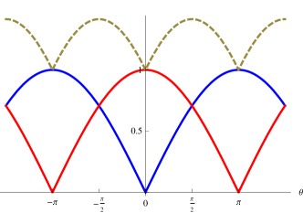
Figure 1: The blue and red lines represent $\left|\cos\frac{\theta}{2}\right|$ and $\left|\sin\frac{\theta}{2}\right|$ separately, and the dashed one indicates $\left|\cos\frac{\theta}{2}\right|+\left|\sin\frac{\theta}{2}\right|$ as for $J_{z}=\pm 1/2$. From the picture we can easily see the extremum values of $f(\theta)$ are $\pm\pi$, $\pm\pi/2$ except the trivial value $\theta=0$.

IV.1 Type I BRM

By introducing the maximum of $\ell_{1}$-norm, if we choose $\theta=-\pi/2$ and the corresponding $\varphi=\pi/2$ obtained by Eq. (98), we get

$$A_{\mbox{I }}=\frac{1}{\sqrt{2}}\left(\begin{array}[]{cc}1&1\\ -1&1\end{array}\right),\quad B_{\mbox{I }}=\frac{1}{\sqrt{2}}\left(\begin{array}[]{cc}1&-i\\ -i&1\end{array}\right).$$

Braid relation will be still valid after a same constant unitary transformation is acted on the matrices $A_{\mbox{I}}$ and $B_{\mbox{I}}$. Using the unitary transformation $V=\frac{1}{\sqrt{2}}\left(\begin{array}[]{cc}1&i\\ i&1\end{array}\right)$ to make matrix $A_{\mbox{I}}$ diagonal:

$$A^{\prime}_{\mbox{I}} =VA_{\mbox{I}}V^{\dagger}=e^{-i\pi/4}\left(\begin{array}[]{cc}1&0\\ 0&i\end{array}\right),$$ (114)

$$B^{\prime}_{\mbox{I}} =VB_{\mbox{I}}V^{\dagger}=\frac{1}{\sqrt{2}}\left(\begin{array}[]{cc}1&-i\\ -i&1\end{array}\right),$$ (117)

It is the same as Eq. (75) except an overall phase factor. Correspondingly, the YBE has the form

$$A(\theta_{1})B(\theta_{2},\varphi=\frac{\pi}{2})A(\theta_{3})=B(\theta_{3},\varphi=\frac{\pi}{2})A(\theta_{2})B(\theta_{1},\varphi=\frac{\pi}{2}),$$ (118)

and the spectral parameter $\theta$ should satisfy the relation[10]

$$\tan\frac{\theta_{2}}{2} =\frac{\tan\frac{\theta_{1}}{2}+\tan\frac{\theta_{3}}{2}}{1+\tan\frac{\theta_{1}}{2}\tan\frac{\theta_{3}}{2}}.$$ (119)

By setting $u=\tan\frac{\theta}{2}$, this is just the additivity rule of Lorentz velocity ($c=1$).

IV.2 Type II BRM

Now we substitute $\theta=\pi$ and corresponding $\varphi=2\pi/3$ which help the $\ell_{1}$-norm of $D^{1/2}(\theta,\varphi)$ to achieve minimum, we obtain

$$A_{\mbox{II }}=\frac{1}{\sqrt{2}}\left(\begin{array}[]{cc}0&-1\\ 1&0\end{array}\right),\quad B_{\mbox{II }}=\frac{1}{\sqrt{2}}\left(\begin{array}[]{cc}0&-e^{-2i\pi/3}\\ e^{2i\pi/3}&0\end{array}\right).$$

Taking the same unitary transformation as for type I, we have

$$A^{\prime}_{\mbox{II}} =VA_{\mbox{II}}V^{\dagger}=(-i)\left(\begin{array}[]{cc}-1&0\\ 0&1\end{array}\right),$$ (122)

$$B^{\prime}_{\mbox{II}} =VB_{\mbox{II}}V^{\dagger}=(-\frac{i}{2})\left(\begin{array}[]{cc}1&-\sqrt{3}\\ -\sqrt{3}&-1\end{array}\right).$$ (125)

The same result is obtained as Eq. (80) except the overall factor $(-i)$. The corresponding YBE relation reads

$$A(\theta_{1})B(\theta_{2},\varphi=\frac{2\pi}{3})A(\theta_{3})=B(\theta_{3},\varphi=\frac{2\pi}{3})A(\theta_{2})B(\theta_{1},\varphi=\frac{2\pi}{3}),$$ (126)

and the spectral parameters should satisfy the relation for $u=\tan\frac{\theta}{2}$

$$u_{2} =u_{1}+u_{3}.$$ (127)

This is just the additivity rule of Galileo velocity .

When $\theta=0$, $A$ becomes a unit matrix, i.e., it is trivial. As concerned to $\theta=-\pi$, $\pi/2$, we can substitute corresponding $\varphi=-2\pi/3$, $-\pi/2$ into Eqs. (101) and (104). The results will just be the transposition of the earlier matrices. If we change the order of original natural basis and the entangled states basis, i.e., $(\left|2\right\rangle,\left|1\right\rangle)$ and $(\left|E_{2}\right\rangle,\left|E_{1}\right\rangle)$, the rotation transformation matrix will also be the transposition of the original one.

$$\left(\begin{array}[]{c}\left|E_{2}\right\rangle\\ \left|E_{1}\right\rangle\end{array}\right) =\left(\begin{array}[]{cc}\cos\frac{\theta}{2}&-\sin\frac{\theta}{2}e^{-i\varphi}\\ \sin\frac{\theta}{2}e^{i\varphi}&\cos\frac{\theta}{2}\end{array}\right)^{T}\left(\begin{array}[]{c}\left|2\right\rangle\\ \left|1\right\rangle\end{array}\right).$$

Everything changes to its transposition, they are still consistent. Subsequently we just concentrate on the cases $\theta=\pi/2$ and $\pi$.

In this way, we present that $\ell_{1}$-norm extremum can assist to determine which $\theta$ and $\varphi$ have physical meanings. Overall, the first type of BRM is related to the anyons and entangled states, and the matrices are chosen by setting $\theta=\pi/2$ and $\varphi=\pi/2$. The second type is connected to fermions and bosons, and the BRM are chosen by setting $\theta=\pi$ and $\varphi=2\pi/3$. It is very interesting that the two types of BRM, which really exist in physics, are just given by the extremum of $\ell_{1}$-norm of the D-function:

maximizing $$\sum_{M=-1/2}^{1/2}\left|D_{MM^{\prime}}^{1/2}(\theta,\varphi)\right|\mbox{ to get type I BRM},$$

minimizing $$\sum_{M=-1/2}^{1/2}\left|D_{MM^{\prime}}^{1/2}(\theta,\varphi)\right|\mbox{ to get type II BRM}.$$

In principle, the discussion for $j=1/2$ can be extended to any dimensional spinor representations, see the appendix C.

V Motivation of using $\ell_{1}$-norm

In our knowledge, up to now, there is no physical interpretation of $\ell_{1}$-norm in QM, but in recent developments in the information field, there has been strong motivation to take $\ell_{1}$-norm into account.

There is a rapidly growing interest in the nonlinear sampling in information theory, which is often referred to Compressive Sensing (C-S) 22 ; 23 ; 24 . It has had many applications to information, digital sensors and computer tomography (CT) 24 . To explain C-S, let us consider a simple example. Suppose the Fourier image of a signal $f(t)\ (t=n\frac{T}{N},n=1,2,\cdots,N)$ is $\tilde{f}(\omega)=\sum_{i=1}^{k}\alpha_{i}\delta(\omega-\omega_{i})$. If $k\ll N$, the signal is called “sparse”. If a signal is sparse, then much less measurements $y$ may be made to recover $f(t)=x$. Suppose measuring matrix $\Phi$ is $M\times N$ matrix ($M\thickapprox k\log N\ll N$, where $k$ is “sparsity”) , i.e., $y=\Phi x$. To recover $x$ ($N$ components), we can only measure $M$ data. Obviously, for given $y$ to find $x$ is an ill-posted problem because $\Phi$ does not have the inverse. However, the C-S tells that the recovery of $f(t)=x$ consists in 23

$$\mbox{minimize }\left\|x\right\|_{\ell_{1}} \quad\mbox{subject to }y=\Phi x.$$ (128)

The $\ell_{1}$-norm plays the crucial role in Eq. (128). Through this example, we can learn that the minimization of $\ell_{1}$-norm can be used to determine some important physical quantities. In Refs.25 ; 26 the C-S theory has been used to calculate density matrix. However, so far the concept of $\ell_{1}$-norm is not emphasized in quantum information theory.

In Sec. IV, we have discussed one possible usage of $\ell_{1}$-norm related to QM because of the important application of $\ell_{1}$-norm in information theory. It is reasonable to think there may be a deep connection between $\ell_{1}$-norm and QM.

VI Physical example related to YBE

In appendix A we have shown that the matrix forms of the two types of 2D YBE are based on the basis $\left|e_{1}\right\rangle$ and $\left|e_{2}\right\rangle$. With this knowledge we can derive the basis of $A(\theta)$ and $B(\theta)$, which satisfy

$$\left(\begin{array}[]{c}\left|e_{1}^{\prime}\right\rangle\\ \left|e_{2}^{\prime}\right\rangle\end{array}\right) =V\left(\begin{array}[]{c}\left|e_{1}\right\rangle\\ \left|e_{2}\right\rangle\end{array}\right),$$

more specifically

$$\left|e_{1}^{\prime}\right\rangle =\frac{1}{\sqrt{2}}\left(\left|e_{1}\right\rangle+i\left|e_{2}\right\rangle\right),$$

$$\left|e_{2}^{\prime}\right\rangle =\frac{1}{\sqrt{2}}\left(i\left|e_{1}\right\rangle+\left|e_{2}\right\rangle\right).$$

After finding out their connections with $\left|e_{1}\right\rangle$ and $\left|e_{2}\right\rangle$, we can use the graph technique to show the operators related to D-function. Here we confirm that $\left|e_{1}^{\prime}\right\rangle$ and $\left|e_{2}^{\prime}\right\rangle$ are nothing but the two basis of SU(2) algebra. Similar to atomic physics, we define three operators:

$$J_{+}= \left|e_{1}^{\prime}\right\rangle\left\langle e_{2}^{\prime}\right|,\quad J_{-}=\left|e_{2}^{\prime}\right\rangle\left\langle e_{1}^{\prime}\right|,$$

$$J_{z}= \frac{1}{2}\left(\left|e_{1}^{\prime}\right\rangle\left\langle e_{1}^{\prime}\right|-\left|e_{2}^{\prime}\right\rangle\left\langle e_{2}^{\prime}\right|\right).$$

Representing the operators as graph

$$J_{+} =\frac{1}{2}\left(\left|e_{1}\right\rangle+i\left|e_{2}\right\rangle\right)\left(i\left|e_{1}\right\rangle+\left|e_{2}\right\rangle\right)$$

$$=\frac{1}{2}\Big{[}\left(\left|e_{2}\right\rangle\left\langle e_{1}\right|+\left|e_{1}\right\rangle\left\langle e_{2}\right|\right)$$

$$\quad+i\left(-\left|e_{1}\right\rangle\left\langle e_{1}\right|+\left|e_{2}\right\rangle\left\langle e_{2}\right|\right)\Big{]}$$

$$=\frac{1}{2}\Bigg{[}\frac{1}{d\sqrt{d^{2}-1}}\left(\raisebox{-0.4pt}{\includegraphics[height=28.45274pt]{21}}+\raisebox{-0.4pt}{\includegraphics[height=28.45274pt]{12}}-\frac{2}{d}\raisebox{-0.4pt}{\includegraphics[height=28.45274pt]{22}}\right)$$

$$\quad+\frac{i}{d^{2}-1}\left(\raisebox{-0.4pt}{\includegraphics[height=28.45274pt]{11}}-\frac{1}{d}\raisebox{-0.4pt}{\includegraphics[height=28.45274pt]{21}}-\frac{1}{d}\raisebox{-0.4pt}{\includegraphics[height=28.45274pt]{12}}+\frac{-d^{2}+2}{d^{2}}\raisebox{-0.4pt}{\includegraphics[height=28.45274pt]{22}}\right)\Bigg{]},$$

$$J_{-} =\frac{1}{2}\Big{[}\left(\left|e_{2}\right\rangle\left\langle e_{1}\right|+\left|e_{1}\right\rangle\left\langle e_{2}\right|\right)$$

$$\quad+i\left(\left|e_{1}\right\rangle\left\langle e_{1}\right|-\left|e_{2}\right\rangle\left\langle e_{2}\right|\right)\Big{]}$$

$$=\frac{1}{2}\Bigg{[}\frac{1}{d\sqrt{d^{2}-1}}\left(\raisebox{-0.4pt}{\includegraphics[height=28.45274pt]{21}}+\raisebox{-0.4pt}{\includegraphics[height=28.45274pt]{12}}-\frac{2}{d}\raisebox{-0.4pt}{\includegraphics[height=28.45274pt]{22}}\right)$$

$$\quad-\frac{i}{d^{2}-1}\left(\raisebox{-0.4pt}{\includegraphics[height=28.45274pt]{11}}-\frac{1}{d}\raisebox{-0.4pt}{\includegraphics[height=28.45274pt]{21}}-\frac{1}{d}\raisebox{-0.4pt}{\includegraphics[height=28.45274pt]{12}}+\frac{-d^{2}+2}{d^{2}}\raisebox{-0.4pt}{\includegraphics[height=28.45274pt]{22}}\right)\Bigg{]},$$

$$J_{z} =\frac{i}{2}\left(\left|e_{2}\right\rangle\left\langle e_{1}\right|-\left|e_{1}\right\rangle\left\langle e_{2}\right|\right)$$

$$=\frac{i}{2d\sqrt{d^{2}-1}}\left(\raisebox{-0.4pt}{\includegraphics[height=28.45274pt]{12}}-\raisebox{-0.4pt}{\includegraphics[height=28.45274pt]{21}}\right).$$

Using graph technique, we can verify that

$$\left[J_{z},\ J_{\pm}\right] =\pm J_{\pm},$$

$$\left[J_{+},\ J_{-}\right] =2J_{z}.$$

Noting

$$J^{2} =\frac{1}{2}\left(J_{+}J_{-}+J_{-}J_{+}\right)+J_{z}J_{z}$$

$$=\frac{3}{4}\left(\left|e_{1}^{\prime}\right\rangle\left\langle e_{1}^{\prime}\right|+\left|e_{2}^{\prime}\right\rangle\left\langle e_{2}^{\prime}\right|\right)$$

$$=\frac{3}{4}\left(\left|e_{1}\right\rangle\left\langle e_{1}\right|+\left|e_{2}\right\rangle\left\langle e_{2}\right|\right)$$

$$=\frac{3}{4}\frac{1}{d^{2}-1}\left(\raisebox{-0.4pt}{\includegraphics[height=28.45274pt]{11}}-\frac{1}{d}\raisebox{-0.4pt}{\includegraphics[height=28.45274pt]{21}}-\frac{1}{d}\raisebox{-0.4pt}{\includegraphics[height=28.45274pt]{12}}+\raisebox{-0.4pt}{\includegraphics[height=28.45274pt]{22}}\right),$$

it is easy to prove that

$$J^{2} \left|e_{i}^{\prime}\right\rangle=\frac{3}{4}\left|e_{i}^{\prime}\right\rangle.$$

Also we have

$$\left(J_{+}\right)^{2} =\left(J_{-}\right)^{2}=0,$$

$$J_{z}\left|e_{1}^{\prime}\right\rangle =\frac{1}{2}\left|e_{1}^{\prime}\right\rangle,$$

$$J_{z}\left|e_{2}^{\prime}\right\rangle =-\frac{1}{2}\left|e_{2}^{\prime}\right\rangle.$$

These calculations let us see that $\left|e_{1}^{\prime}\right\rangle$ and $\left|e_{2}^{\prime}\right\rangle$ are nothing but the two basis of SU(2) algebra.

The 2-states can be understood in terms of the Cooper pair of superconductivity. Through the mean field approximation, the four-fermion interaction

$$H =\sum_{\vec{k}}\varepsilon_{\vec{k}}a_{\vec{k}}^{+}a_{\vec{k}}+\sum_{\sigma=\pm}A_{\vec{k}\vec{k}^{\prime}}a_{-\vec{k}\sigma}^{+}a_{\vec{k}\sigma}^{+}a_{\vec{k}\sigma}a_{-\vec{k}\sigma}$$

reduces to

$$H_{0} =\sum_{\vec{k}}H_{\vec{k}}^{0},$$

where

$$H_{\vec{k}}^{0} =\varepsilon_{\vec{k}}J_{z}^{\vec{k}}+\frac{1}{2}\Delta_{\vec{k}}^{*}J_{-}^{\vec{k}}+\frac{1}{2}\Delta_{\vec{k}}^{*}J_{+}^{\vec{k}},$$

$\Delta_{\vec{k}}=\sum_{\vec{k}^{\prime}}A_{\vec{k}\vec{k}^{\prime}}\left\langle a_{\vec{k}^{\prime}\downarrow},a_{-\vec{k}\uparrow}\right\rangle$ and $J_{\pm}^{\vec{k}}$, $J_{z}^{\vec{k}}$ satisfy the SU(2)-algebra. The operator $D(\xi)$ can be used to diagonalize the $H_{\vec{k}}$ for a fixed $\vec{k}$:

$$D(\xi)=e^{\xi J_{+}-\xi^{*}J_{-}} =e^{\tau J_{+}}e^{\ln(1+|\tau|^{2})J_{z}}e^{-\tau^{*}J_{-}},$$

$$D(\xi)H_{\vec{k}}D^{\dagger}(\xi)=E_{\vec{k}}J_{z}, \quad E_{\vec{k}}=\left(\varepsilon_{\vec{k}}^{2}+\left|\Delta_{\vec{k}}\right|^{2}\right)^{1/2},$$

$$\Delta_{\vec{k}}=\left|\Delta_{\vec{k}}\right|e^{i\varphi/2}, \quad\tan\theta_{\vec{k}}=\frac{\left|\Delta_{\vec{k}}\right|}{\varepsilon_{\vec{k}}},$$

$$\xi=\frac{\theta}{2}e^{-i\varphi}, \quad\tau=e^{-i\varphi}\tan\frac{\theta}{2}.$$

where $J_{+}$, $J_{-}$ and $J_{z}$ are angular momentum operators. In terms of the fermion operators

$$J_{\vec{k}}^{+}=a_{-\vec{k}\downarrow}^{+} a_{\vec{k}\uparrow}^{+},\quad J_{\vec{k}}^{-}=a_{\vec{k}\uparrow}a_{-\vec{k}\downarrow},$$

$$J_{\vec{k}}^{z}=\frac{1}{2} \left(n_{\vec{k}\uparrow}+n_{-\vec{k}\downarrow}-1\right),$$

and defining

$$J_{-}^{\vec{k}} \left|0\right\rangle_{\vec{k}}=0\quad\left|\xi\right\rangle_{\vec{k}}=e^{\xi J_{+}^{k}-\xi*J_{-}^{k}}\left|0,0\right\rangle_{\vec{k}}$$

where $\left|0,0\right\rangle_{\vec{k}}$ is the eigen state of $\left|n_{\vec{k}\uparrow}=0,n_{-\vec{k}\downarrow}=0\right\rangle$, then

$$\left|\xi\right\rangle_{\vec{k}} =e^{\tau J_{+}}e^{\ln(1+|\tau|^{2})J_{z}}e^{-\tau^{*}J_{-}}\left|0,0\right\rangle_{\vec{k}}$$

$$=e^{\tau J_{+}}e^{\ln(1+|\tau|^{2})J_{z}}\left|0,0\right\rangle_{\vec{k}}$$

$$=\frac{1}{\sqrt{1+|\tau|^{2}}}\left(\left|0,0\right\rangle_{\vec{k}}+\tau\left|1,1\right\rangle_{\vec{k}}\right),$$

where $\left|0,0\right\rangle_{k}=|n_{\vec{k}\uparrow}=0,n_{-\vec{k}\downarrow}=0\rangle$ and $\left|1,1\right\rangle_{k}=|n_{\vec{k}\uparrow}=1,n_{-\vec{k}\downarrow}=1\rangle$, i.e., $J_{z}|0,0\rangle=-\frac{1}{2}|0,0\rangle$ and $J_{z}|1,1\rangle=+\frac{1}{2}|1,1\rangle$. It is easy to find

$$D(\xi)\left(\begin{array}[]{c}\left|0,0\right\rangle\\ \left|1,1\right\rangle\end{array}\right) =\left(\begin{array}[]{cc}\cos\frac{\theta}{2}&\sin\frac{\theta}{2}e^{-i\varphi}\\ -\sin\frac{\theta}{2}e^{i\varphi}&\cos\frac{\theta}{2}\end{array}\right)\left(\begin{array}[]{c}\left|0,0\right\rangle\\ \left|1,1\right\rangle\end{array}\right),$$

namely $|0,0\rangle$ and $|1,1\rangle$ can be served as $|2\rangle$ and $|1\rangle$ in section IV. Suppose $\theta$ and $\varphi$ are taken to be $(-\pi/2,\pi/2)$ and $(\pi,2\pi/3)$, respectively. It yields the same matrix as given by (75). The ground energy $E_{\vec{k}}$ degenerates to $\varphi$, which can be detected through Josephson current. With this sense, CS may be served as simulation of YBE for any $\Delta_{\vec{k}}$, i.e., $\theta_{\vec{k}}$ with the corresponding $\varphi_{\vec{k}}$.

VII Examples of $J=1$ and $J=3/2$

In appendix C it has been provided evidence that for arbitrary $j=1/2,1,3/2,\cdots$ etc., $\sum_{M^{\prime}=-J}^{M^{\prime}=J}\left|D_{MM^{\prime}}^{J}(\theta,\varphi)\right|$ can reach its extreme value when $\theta=-\pi,-\pi/2,0,\pi/2,\pi$ ($\theta\in[-\pi,\pi]$). This result can generalize the result for $J=1/2$ and the corresponding $2\times 2$ BRM. In this section we shall calculate the $\ell_{1}$-norm of $D_{MM^{\prime}}^{J}(\theta,\varphi)$ for $J=1$ and $J=3/2$, and demonstrate that the extremum of $\ell_{1}$-norm lead to the two types of BRM.

VII.1 $J=1$

We take the $\ell_{1}$-norm of every row of the D-function $D_{MM^{\prime}}^{1}(\theta,\varphi)$. From Eqs. (169) and (177), it can be derived that $\left|D_{MM^{\prime}}^{1}(\theta,\varphi)\right|=\left|d_{MM^{\prime}}^{1}(\theta)\right|$, and the first and third row share the same results, therefor we just concentrate on the first two rows. We can prove that for $\theta\in[-\pi,\pi]$, $\ell_{1}$-norm can achieve its extremum value when $\theta=-\pi,-\pi/2,0,\pi/2,\pi$. For detailed calculations, please refer to appendix C. The maximum and minimum can be seen easily from pictures 2 and 3.

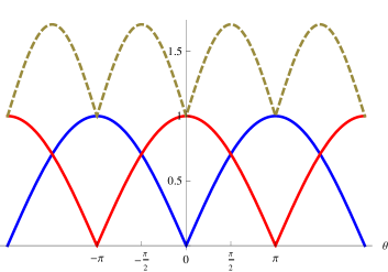
Figure 2: The blue and red lines represent $\left|\cos\frac{\theta}{2}\right|$ and $\left|\sin\frac{\theta}{2}\right|$ separately, and the dashed one indicates $f(\theta)_{1}^{1}=\left|(1+\cos\theta)/2\right|+\left|-\sin\theta/\sqrt{2}\right|+\left|(1-\cos\theta)/2\right|$, as for $J_{z}=\pm 1$ states. From the picture we can easily see the extremum values of $f(\theta)_{1}^{1}$ and the corresponding $\theta$.

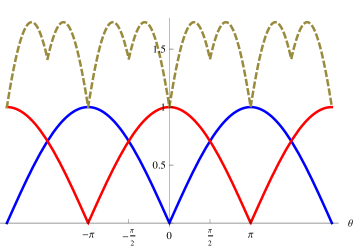
Figure 3: The blue and red lines represent $\left|\cos\frac{\theta}{2}\right|$ and $\left|\sin\frac{\theta}{2}\right|$ separately, and the dashed one indicates $f(\theta)_{2}^{1}=\left|\sin\theta/\sqrt{2}\right|+\left|\cos\theta\right|+\left|-\sin\theta/\sqrt{2}\right|$ as for $J_{z}=0$ state. From the picture we can easily see the extremum values of $f(\theta)_{2}^{1}$ and the corresponding $\theta$.

Although Fig. (3) has more extremum points than Fig. (2), there are just five points that figures 2 and 3 share together. From the view of point in Fig. (2), we can still choose $\theta=\pi/2$ and $\pi$ to find out two types of BRM.

1. Substituting $\theta=\pi/2$ and $\varphi=\pi/2$ into Eqs. (169) and (177), we get

   $$A_{\mbox{I}}^{1}=\left(\begin{array}[]{ccc}\frac{1}{2}&-\frac{1}{\sqrt{2}}&\frac{1}{2}\\ \frac{1}{\sqrt{2}}&0&-\frac{1}{\sqrt{2}}\\ \frac{1}{2}&\frac{1}{\sqrt{2}}&\frac{1}{2}\end{array}\right),\quad B_{\mbox{I}}^{1}=\left(\begin{array}[]{ccc}\frac{1}{2}&\frac{i}{\sqrt{2}}&-\frac{1}{2}\\ \frac{i}{\sqrt{2}}&0&\frac{i}{\sqrt{2}}\\ -\frac{1}{2}&\frac{i}{\sqrt{2}}&\frac{1}{2}\end{array}\right).$$

   After taking the unitary transformation

   $$\widetilde{A_{\mbox{I}}^{1}} =T^{\dagger}A_{\mbox{I}}^{1}T=\left(\begin{array}[]{ccc}-i&0&0\\ 0&1&0\\ 0&0&i\end{array}\right),$$

   $$\widetilde{B_{\mbox{I}}^{1}} =T^{\dagger}B_{\mbox{I}}^{1}T=\left(\begin{array}[]{ccc}\frac{1}{2}&\frac{1}{\sqrt{2}}&\frac{1}{2}\\ -\frac{1}{\sqrt{2}}&0&\frac{1}{\sqrt{2}}\\ \frac{1}{2}&-\frac{1}{\sqrt{2}}&\frac{1}{2}\end{array}\right),$$

   where $T=\left(\begin{array}[]{ccc}\frac{1}{2}&\frac{1}{\sqrt{2}}&\frac{1}{2}\\ \frac{i}{\sqrt{2}}&0&-\frac{i}{\sqrt{2}}\\ -\frac{1}{2}&\frac{1}{\sqrt{2}}&-\frac{1}{2}\end{array}\right).$ This is the $3\times 3$ type I BRM.

2. Substituting $\theta=\pi$ and $\varphi=2\pi/3$ into Eqs. (169) and (177), we get

   $$A_{\mbox{II}}^{1}=\left(\begin{array}[]{ccc}0&0&1\\ 0&-1&0\\ 1&0&0\end{array}\right),\quad B_{\mbox{II}}^{1}=\left(\begin{array}[]{ccc}0&0&e^{2i\pi/3}\\ 0&-1&0\\ e^{-2i\pi/3}&0&0\end{array}\right).$$

   After taking the same unitary transformation

   $$\widetilde{A_{\mbox{II}}^{1}} =\left(\begin{array}[]{ccc}-1&0&0\\ 0&1&0\\ 0&0&-1\end{array}\right),\quad\widetilde{B_{\mbox{II}}^{1}}=\left(\begin{array}[]{ccc}-\frac{1}{4}&i\frac{\sqrt{6}}{4}&\frac{3}{4}\\ -i\frac{\sqrt{6}}{4}&-\frac{1}{2}&-i\frac{\sqrt{6}}{4}\\ \frac{3}{4}&i\frac{\sqrt{6}}{4}&-\frac{1}{4}\end{array}\right).$$

   This is the $3\times 3$ type II BRM.

Both types of BRM satisfy the braid relation $\widetilde{A^{1}}\widetilde{B^{1}}\widetilde{A^{1}}=\widetilde{B^{1}}\widetilde{A^{1}}\widetilde{B^{1}}$. It should be noted that for vector solutions ($J=1,2,\cdots$) when $\theta=\pm\pi/2$, the $\ell_{1}$-norm of D-function matrices may achieve minimum value, not maximum as the case for spinor solutions ($J=1/2$, $3/2$, $\cdots$).

A valuable attention is that for $J=1$ the maximum at $\pm\pi/2$ and minimums at $\pm\pi$ for states $J_{z}=\pm 1$ are the same, but for $J_{z}=0$ state the $\pm\pi/2$ are the minimum. This state should be singleted, the physical interpretation is chiral photon. This picture does not occur in spinors, i.e., for $J$ is half integers.

VII.2 $J=3/2$

We take the $\ell_{1}$-norm of every row of the D-function $D_{MM^{\prime}}^{3/2}(\theta,\varphi)$. From Eqs. (182) and (187) it can be derived that $\left|D_{MM^{\prime}}^{3/2}(\theta,\varphi)\right|=\left|d_{MM^{\prime}}^{3/2}(\theta)\right|$, also the first and third row have the same results. We just concentrate on the first two rows. We can also prove that for $\theta\in[-\pi,\pi]$, $\ell_{1}$-norm can achieve its extremum value when $\theta=-\pi,-\pi/2,0,\pi/2,\pi$. The maximum and minimum can be seen easily from pictures 4 and 5.

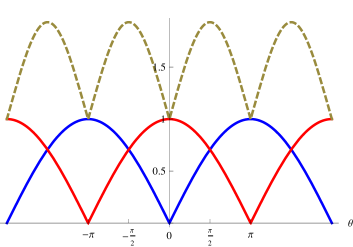
Figure 4: The blue and red lines represent $\left|\cos\frac{\theta}{2}\right|$ and $\left|\sin\frac{\theta}{2}\right|$ separately, and the dashed one indicates $f(\theta)_{1}^{3/2}=\left|\cos^{3}\frac{\theta}{2}\right|+\left|-\sqrt{3}\sin\frac{\theta}{2}\cos^{2}\frac{\theta}{2}\right|+\left|\sqrt{3}\sin^{2}\frac{\theta}{2}\cos\frac{\theta}{2}\right|+\left|-\sin^{3}\frac{\theta}{2}\right|$ as for $J_{z}=\pm 3/2$. From the picture we can easily see the extremum values of $f(\theta)_{1}^{1}$ and the corresponding $\theta$.

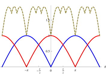
Figure 5: The blue and red lines represent $\left|\cos\frac{\theta}{2}\right|$ and $\left|\sin\frac{\theta}{2}\right|$ separately, and the dashed one indicates $f(\theta)_{2}^{3/2}=\left|\sqrt{3}\sin\frac{\theta}{2}\cos^{2}\frac{\theta}{2}\right|+\left|\cos\frac{\theta}{2}\left(3\cos^{2}\frac{\theta}{2}-2\right)\right|+\left|\sin\frac{\theta}{2}\left(3\sin^{2}\frac{\theta}{2}-2\right)\right|+\left|\sqrt{3}\sin^{2}\frac{\theta}{2}\cos\frac{\theta}{2}\right|$ as for $J_{z}=\pm 1/2$. From the picture we can easily see the extremum values of $f(\theta)_{2}^{1}$ and the corresponding $\theta$.

Although Fig. (5) has more extremum points than Fig. (4), there are just five points that they share together. From the view of point in Fig. (4), we can choose $\theta=\pi/2$ and $\pi$ to find the two types of BRM.

1. Substituting $\theta=\pi/2$ and $\varphi=\pi/2$ into Eqs. (182) and (187), we get

   $$A_{\mbox{I}}^{3/2} =\left(\begin{array}[]{cccc}\frac{1}{2\sqrt{2}}&-\frac{\sqrt{6}}{4}&\frac{\sqrt{6}}{4}&-\frac{1}{2\sqrt{2}}\\ \frac{\sqrt{6}}{4}&-\frac{1}{2\sqrt{2}}&-\frac{1}{2\sqrt{2}}&\frac{\sqrt{6}}{4}\\ \frac{\sqrt{6}}{4}&\frac{1}{2\sqrt{2}}&-\frac{1}{2\sqrt{2}}&-\frac{\sqrt{6}}{4}\\ \frac{1}{2\sqrt{2}}&\frac{\sqrt{6}}{4}&\frac{\sqrt{6}}{4}&\frac{1}{2\sqrt{2}}\end{array}\right),$$

   $$B_{\mbox{I}}^{3/2} =\left(\begin{array}[]{cccc}\frac{1}{2\sqrt{2}}&i\frac{\sqrt{6}}{4}&-\frac{\sqrt{6}}{4}&-\frac{i}{2\sqrt{2}}\\ i\frac{\sqrt{6}}{4}&-\frac{1}{2\sqrt{2}}&\frac{i}{2\sqrt{2}}&-\frac{\sqrt{6}}{4}\\ -\frac{\sqrt{6}}{4}&\frac{i}{2\sqrt{2}}&-\frac{1}{2\sqrt{2}}&i\frac{\sqrt{6}}{4}\\ -\frac{i}{2\sqrt{2}}&-\frac{\sqrt{6}}{4}&i\frac{\sqrt{6}}{4}&\frac{1}{2\sqrt{2}}\end{array}\right).$$

   After taking the unitary transformation

   $$\widetilde{A_{\mbox{I}}^{3/2}} =U^{\dagger}A_{\mbox{I}}^{1}U=\left(\begin{array}[]{cccc}-e^{i\pi/4}&0&0&0\\ 0&e^{i\pi/4}&0&0\\ 0&0&e^{-i\pi/4}&0\\ 0&0&0&-e^{-i\pi/4}\end{array}\right),$$

   $$\widetilde{B_{\mbox{I}}^{3/2}} =U^{\dagger}B_{\mbox{I}}^{1}U=\left(\begin{array}[]{cccc}\frac{1}{2\sqrt{2}}&\frac{\sqrt{6}}{4}&-\frac{\sqrt{6}}{4}&-\frac{1}{2\sqrt{2}}\\ \frac{\sqrt{6}}{4}&-\frac{1}{2\sqrt{2}}&\frac{1}{2\sqrt{2}}&-\frac{\sqrt{6}}{4}\\ \frac{\sqrt{6}}{4}&-\frac{1}{2\sqrt{2}}&-\frac{1}{2\sqrt{2}}&\frac{\sqrt{6}}{4}\\ \frac{1}{2\sqrt{2}}&\frac{\sqrt{6}}{4}&\frac{\sqrt{6}}{4}&\frac{1}{2\sqrt{2}}\end{array}\right),$$

   where $U=\left(\begin{array}[]{cccc}\frac{i}{2\sqrt{2}}&i\frac{\sqrt{6}}{4}&-i\frac{\sqrt{6}}{4}&-\frac{i}{2\sqrt{2}}\\ -\frac{\sqrt{6}}{4}&\frac{1}{2\sqrt{2}}&\frac{1}{2\sqrt{2}}&-\frac{\sqrt{6}}{4}\\ -i\frac{\sqrt{6}}{4}&\frac{i}{2\sqrt{2}}&-\frac{i}{2\sqrt{2}}&i\frac{\sqrt{6}}{4}\\ \frac{1}{2\sqrt{2}}&\frac{\sqrt{6}}{4}&\frac{\sqrt{6}}{4}&\frac{1}{2\sqrt{2}}\end{array}\right).$ This is the $4\times 4$ type I BRM.

2. Substituting $\theta=\pi$ and $\varphi=2\pi/3$ into Eqs. (182) and (187), we get

   $$A_{\mbox{II}}^{3/2} =\left(\begin{array}[]{cccc}0&0&0&-1\\ 0&0&1&0\\ 0&-1&0&0\\ 1&0&0&0\end{array}\right),$$

   $$B_{\mbox{II}}^{3/2} =\left(\begin{array}[]{cccc}0&0&0&-1\\ 0&0&e^{-2i\pi/3}&0\\ 0&-e^{2i\pi/3}&0&0\\ 1&0&0&0\end{array}\right).$$

   After taking the same unitary transformation

   $$\widetilde{A_{\mbox{II}}^{3/2}} =\left(\begin{array}[]{cccc}i&0&0&0\\ 0&i&0&0\\ 0&0&-i&0\\ 0&0&0&-i\end{array}\right),$$

   $$\widetilde{B_{\mbox{II}}^{3/2}} =\left(\begin{array}[]{cccc}-\frac{i}{8}&i\frac{3\sqrt{3}}{8}&\frac{3}{8}&-\frac{3\sqrt{3}}{8}\\ i\frac{3\sqrt{3}}{8}&i\frac{5}{8}&-\frac{\sqrt{3}}{8}&\frac{3}{8}\\ -\frac{3}{8}&\frac{\sqrt{3}}{8}&-i\frac{5}{8}&-i\frac{3\sqrt{3}}{8}\\ \frac{3\sqrt{3}}{8}&-\frac{3}{8}&-i\frac{3\sqrt{3}}{8}&\frac{i}{8}\end{array}\right).$$

   This is the $4\times 4$ type II BRM.

Both types of BRM satisfy the braid relation $\widetilde{A^{3/2}}\widetilde{B^{3/2}}\widetilde{A^{3/2}}=\widetilde{B^{3/2}}\widetilde{A^{3/2}}\widetilde{B^{3/2}}$.

The physical interpretation of the $3\times 3$ and $4\times 4$ BRM remains to be discovered. We want to emphasize that based on the proof in appendix C we can further calculate $n\times n$ BRM ($n=2J+1$ is an arbitrary integer). In this section, we just give the two simplest examples $n=3$ and $4$ to show the difference between spinors and vectors.

VIII Conclusion

In quantum mechanics, we should normalize a wave function, so we are familiar with $\ell_{2}$-norm but not $\ell_{1}$-norm. Considering the important application of the $\ell_{1}$-norm theory in the information theory, we try to introduce the $\ell_{1}$-norm to QM through the three-dimensional rotation transformation for spin system. It turns out that by taking the extremum of $\ell_{1}$-norm of D-functions with $J=1/2$, we can derive the two types of YBE, which have important physical interpretation. One of them is connected with anyons and entangled states while the other is related to the usual low dimensional integrable models.

By the end, we generalize the result to the D-functions with$j=1$, $3/2$ and find out that they have the same property. This result shows there may be a deep connection between $\ell_{1}$-norm and QM, D-functions as well as YBE. The same properties are held for any J being half integers, see appendix C. However, extending the discussions for 2 x 2 and 4 x 4 braiding matrices to any J is a challenge problem.

Appendix A Expressions of the two types of YBE

By using the same calculation method, we can obtain the two explicit types of 2D YBE. We set $\check{R}_{ii+1}(u)=a_{i}(u)I+b_{i}(u)T_{ii+1}$ and act $\breve{R}$ on $\left|e_{1}\right\rangle$ and $\left|e_{2}\right\rangle$; then we have

$$\check{R}_{12}(u)|e_{1}\rangle =[a_{1}(u)+db_{1}(u)]|e_{1}\rangle,$$ (129)

$$\check{R}_{12}(u)|e_{2}\rangle =a_{1}(u)|e_{1}\rangle,$$ (130)

$$\check{R}_{23}(u)|e_{1}\rangle =\left[a_{2}(u)+\frac{b_{2}(u)}{d}\right]|e_{1}\rangle+\epsilon\frac{\sqrt{d^{2}-1}}{d}b_{2}(u)|e_{2}\rangle,$$ (131)

$$\check{R}_{23}(u)|e_{2}\rangle =\epsilon\frac{\sqrt{d^{2}-1}}{d}b_{2}(u)|e_{1}\rangle+\left[a_{2}(u)+\frac{d^{2}-1}{d}b_{2}(u)\right]|e_{2}\rangle.$$ (132)

These should give the 2-D representations of $\check{R}_{12}(u)$ and $\check{R}_{23}(u)$. Defining

$$\begin{array}[]{l}\mathscr{A}_{ij}(u)=\langle e_{i}|\check{R}_{12}(u)|e_{j}\rangle,\\ \mathscr{B}_{ij}(u)=\langle e_{i}|\check{R}_{23}(u)|e_{j}\rangle,\ \ (i,j=1,2).\end{array}$$ (135)

we have

$$\mathscr{A}(u)=\left(\begin{array}[]{cc}a_{1}(u)+db_{1}(u)&0\\ 0&a_{1}(u)\end{array}\right),$$ (138)

$$\mathscr{B}(u)=\left(\begin{array}[]{cc}a_{2}(u)+\frac{b_{2}(u)}{d}&\epsilon\frac{\sqrt{d^{2}-1}}{d}b_{2}(u)\\ \epsilon\frac{\sqrt{d^{2}-1}}{d}b_{2}(u)&a_{2}(u)+\frac{d^{2}-1}{d}b_{2}(u)\end{array}\right).$$ (141)

The YBE should be satisfied for the $1$-D momentum conservation:

$$\mathscr{A}(u)\mathscr{B}(u+v)\mathscr{A}(v)=\mathscr{B}(v)\mathscr{A}(u+v)\mathscr{B}(u).$$ (142)

To simplify the independent relations, we take the special case where

$$a_{1}(u)=a_{2}(u)=a(u),\ \ b_{1}(u)=b_{2}(u)=b(u).$$ (143)

The only constraint equation is simplified to

$$[a(u)b(v)+b(u)a(v)+db(v)b(u)]a(u+v)$$

$$=[a(v)a(u)-b(u)b(v)]b(u+v).$$

Setting

$$a(u) =\rho(u),\quad b(u)=\rho(u)G(u),$$

the YBE leads to

$$G(u)=\frac{u}{\gamma-u},$$ (144)

for $d=2$ ($\gamma$ is arbitrary),

$$\mathscr{A}(u)=\rho(u)\left(\begin{array}[]{cc}\frac{\gamma+u}{\gamma-u}&0\\ 0&1\end{array}\right),$$ (147)

$$\mathscr{B}(u)=\frac{\rho(u)}{2(\gamma-u)}\left(\begin{array}[]{cc}2\gamma-u&\epsilon\sqrt{3}u\\ \epsilon\sqrt{3}u&2\gamma+u\end{array}\right).$$ (150)

This is the second type of 2D YBE, which satisfies the Galileo velocity addition rule as shown in Eq. (127). If we introduce the transformation

$$\frac{\gamma+u}{\gamma-u}\equiv e^{-i\theta}, \quad\rho(u)\equiv e^{i\theta/2},$$

then

$$\rho(u)\frac{u}{\gamma-u}=-i\sin\frac{\theta}{2},\quad \rho(u)\frac{\gamma}{\gamma-u}=\cos\frac{\theta}{2}.$$

We can use these notations to obtain the following matrices

$$\mathscr{A}(u) =\left(\begin{array}[]{cc}e^{-i\theta/2}&0\\ 0&e^{i\theta/2}\end{array}\right)\equiv A^{\prime}(\theta),$$

$$\mathscr{B}(u) =\left(\begin{array}[]{cc}\cos\frac{\theta}{2}+\frac{i}{2}\sin\frac{\theta}{2}&i\frac{\sqrt{3}}{2}\sin\frac{\theta}{2}\\ i\frac{\sqrt{3}}{2}\sin\frac{\theta}{2}&\cos\frac{\theta}{2}-\frac{i}{2}\sin\frac{\theta}{2}\end{array}\right)\equiv B^{\prime}(\theta,\varphi=\frac{2\pi}{3}).$$

By using this notations we have identified the expressions of (108) (111) and (147) (150) except $\theta\to-\theta$.

From Ref. 10 , the first type of 2D YBE, we introduce the transformation

$$\frac{1+\beta^{2}u^{2}+2i\epsilon\beta u}{1+\beta^{2}u^{2}-2i\epsilon\beta u}\equiv e^{-i\theta}, \quad\rho(u)\equiv e^{-i\theta/2},$$

We then obtain the following matrices

$$\mathscr{A}(u) =\left(\begin{array}[]{cc}e^{-i\theta/2}&0\\ 0&e^{i\theta/2}\end{array}\right)\equiv A^{\prime}(\theta),$$

$$\mathscr{B}(u) =\left(\begin{array}[]{cc}\cos\frac{\theta}{2}&-i\sin\frac{\theta}{2}\\ -i\sin\frac{\theta}{2}&\cos\frac{\theta}{2}\end{array}\right)\equiv B^{\prime}(\theta,\varphi=\frac{\pi}{2}).$$

In this way we identify the expressions of (108) (111) and (83) (86) except $\theta\to-\theta$. From the above expressions we see clearly that the matrix form of D-function gives a uniform way to describe the two types of 2D YBE.

Appendix B Matrix form of D-functions

B.1 Notations

The general D-function expression is 20

$$D(\alpha,\beta,\gamma) =e^{-i\alpha J_{z}}e^{-i\beta J_{y}}e^{-i\gamma J_{z}}.$$

However, the D-function we used in this paper has a special property, following Perelomov 27

$$D(\theta,\varphi) =e^{-i\theta\mathbf{m\cdot J}}=e^{\zeta J_{+}-\zeta*J_{-}},$$

where

$$\zeta=-\frac{\theta}{2}e^{-i\varphi}, \quad\mathbf{m}=(-\sin\varphi,\cos\varphi,0),$$ (151)

$\mathbf{J}$ is the angular momentum operator. There is another form of D-function

$$D(n) =e^{nJ_{+}}e^{\ln(1+|n|^{2})J_{z}}e^{-n^{*}J_{-}},$$ (152)

$$n=-\tan\frac{\theta}{2}e^{-i\varphi}$$ (153)

The D-function $D(\theta,\varphi)$ means a rotation of angle $\theta$ about the axis $\mathbf{m}$ which is determined by $\varphi$ as shown in Eq.(151). This specific operator $D(\theta,\varphi)$ was used to generate spin coherent states 27 ; 28 .

It is easy to calculate the relation between $D(\alpha,\beta,\gamma)$ and $D(\theta,\varphi)$, i.e.,

$$\theta =\beta,$$

$$\varphi =\alpha=-\gamma,$$

so

$$D(\theta,\varphi) =e^{-i\varphi J_{z}}e^{-\theta J_{y}}e^{i\varphi Jz}.$$

Then the matrix form of the rotation operator $D(\theta,\varphi)$ would be

$$D_{MM^{\prime}}^{J}(\theta,\varphi) =\left\langle J,M\right|e^{-i\varphi J_{z}}e^{-\theta J_{y}}e^{i\varphi Jz}\left|J,M^{\prime}\right\rangle$$

$$=e^{-i\varphi M}e^{i\varphi M^{\prime}}\left\langle J,M\right|e^{-\theta J_{y}}\left|J,M^{\prime}\right\rangle$$

$$=e^{i\varphi(-M+M^{\prime})}d_{MM^{\prime}}^{J}(\theta).$$ (154)

We need to let matrix $A$ be the same as $d_{MM^{\prime}}^{J}(\theta)$ and matrix $B$ as $D_{MM^{\prime}}^{J}(\theta,\varphi)$. It indicates that $A$ comes from a rotation of angle $\theta$ along the $y$ axis and $B$ comes from the same rotation angle, but along the axis of $(-\sin\varphi,\cos\varphi,0)$, which can be obtained by rotating $y$ of the angle $\varphi$ along $z$ axis.

By choosing $\varphi=0$ in Eq. (154), we get

$$A =D_{MM^{\prime}}^{J}(\theta,\varphi=0)=d_{MM^{\prime}}^{J}(\theta),$$ (155)

so $B$ satisfies

$$B= D_{MM^{\prime}}^{J}(\theta,\varphi)=e^{i\varphi(-M+M^{\prime})}d_{MM^{\prime}}^{J}(\theta).$$ (156)

In Ref. 20 , the explicit forms of $d_{MM^{\prime}}^{J}(\theta)$ had been given.

B.2 Example $J=1/2$

The values of $d_{MM^{\prime}}^{1/2}\left(\theta\right)$ are shown in table 1:

	$\frac{1}{2}$	$-\frac{1}{2}$
$\frac{1}{2}$	$\cos\frac{\theta}{2}$	$-\sin\frac{\theta}{2}$
$-\frac{1}{2}$	$\sin\frac{\theta}{2}$	$\cos\frac{\theta}{2}$

Table 1: Explicit form of $d_{MM^{\prime}}^{1/2}\left(\theta\right)$

Then

$$A =d_{MM^{\prime}}^{1/2}\left(\theta\right)=\left(\begin{array}[]{cc}\cos\frac{\theta}{2}&-\sin\frac{\theta}{2}\\ \sin\frac{\theta}{2}&\cos\frac{\theta}{2}\end{array}\right).$$ (159)

$$B =D_{MM^{\prime}}^{1/2}\left(\theta,\varphi\right)=A\odot\left(\begin{array}[]{cc}1&e^{-i\varphi}\\ e^{i\varphi}&1\end{array}\right)$$ (162)

$$=\left(\begin{array}[]{cc}\cos\frac{\theta}{2}&-\sin\frac{\theta}{2}e^{-i\varphi}\\ \sin\frac{\theta}{2}e^{i\varphi}&\cos\frac{\theta}{2}\end{array}\right),$$ (165)

where $\odot$ means entrywise product.

B.3 Example $J=1$

For $J=1$, following the same procedure, we get

$$A =d_{MM^{\prime}}^{1}\left(\theta\right)=\left(\begin{array}[]{ccc}\frac{1+\cos\theta}{2}&-\frac{\sin\theta}{\sqrt{2}}&\frac{1-\cos\theta}{2}\\ \frac{\sin\theta}{\sqrt{2}}&\cos\theta&-\frac{\sin\theta}{\sqrt{2}}\\ \frac{1-\cos\theta}{2}&\frac{\sin\theta}{\sqrt{2}}&\frac{1+\cos\theta}{2}\end{array}\right),$$ (169)

$$B =D_{MM^{\prime}}^{1}\left(\theta,\varphi\right)=A\odot\left(\begin{array}[]{ccc}1&e^{-i\varphi}&e^{-2i\varphi}\\ e^{i\varphi}&1&e^{-i\varphi}\\ e^{2i\varphi}&e^{i\varphi}&1\end{array}\right)$$ (173)

$$=\left(\begin{array}[]{ccc}\frac{1+\cos\theta}{2}&-\frac{\sin\theta}{\sqrt{2}}e^{-i\varphi}&\frac{1-\cos\theta}{2}e^{-2i\varphi}\\ \frac{\sin\theta}{\sqrt{2}}e^{i\varphi}&\cos\theta&-\frac{\sin\theta}{\sqrt{2}}e^{-i\varphi}\\ \frac{1-\cos\theta}{2}e^{2i\varphi}&\frac{\sin\theta}{\sqrt{2}}e^{i\varphi}&\frac{1+\cos\theta}{2}\end{array}\right).$$ (177)

B.4 Example $J=3/2$

For $J=3/2$, by following the same procedure, we obtain

$$A =d_{MM^{\prime}}^{3/2}\left(\theta\right)=\left(\begin{array}[]{cccc}\cos^{3}\frac{\theta}{2}&-\sqrt{3}\sin\frac{\theta}{2}\cos^{2}\frac{\theta}{2}&\sqrt{3}\sin^{2}\frac{\theta}{2}\cos\frac{\theta}{2}&-\sin^{3}\frac{\theta}{2}\\ \sqrt{3}\sin\frac{\theta}{2}\cos^{2}\frac{\theta}{2}&\cos\frac{\theta}{2}\left(3\cos^{2}\frac{\theta}{2}-2\right)&\sin\frac{\theta}{2}\left(3\sin^{2}\frac{\theta}{2}-2\right)&\sqrt{3}\sin^{2}\frac{\theta}{2}\cos\frac{\theta}{2}\\ \sqrt{3}\sin^{2}\frac{\theta}{2}\cos\frac{\theta}{2}&-\sin\frac{\theta}{2}\left(3\sin^{2}\frac{\theta}{2}-2\right)&\cos\frac{\theta}{2}\left(3\cos^{2}\frac{\theta}{2}-2\right)&-\sqrt{3}\sin\frac{\theta}{2}\cos^{2}\frac{\theta}{2}\\ \sin^{3}\frac{\theta}{2}&\sqrt{3}\sin^{2}\frac{\theta}{2}\cos\frac{\theta}{2}&\sqrt{3}\sin\frac{\theta}{2}\cos^{2}\frac{\theta}{2}&\cos^{3}\frac{\theta}{2}\end{array}\right),$$ (182)

$$B =D_{MM^{\prime}}^{3/2}\left(\theta,\varphi\right)=\left(\begin{array}[]{cccc}\cos^{3}\frac{\theta}{2}&-\sqrt{3}\sin\frac{\theta}{2}\cos^{2}\frac{\theta}{2}e^{-i\varphi}&\sqrt{3}\sin^{2}\frac{\theta}{2}\cos\frac{\theta}{2}e^{-2i\varphi}&-\sin^{3}\frac{\theta}{2}e^{-3i\varphi}\\ \sqrt{3}\sin\frac{\theta}{2}\cos^{2}\frac{\theta}{2}e^{i\varphi}&\cos\frac{\theta}{2}\left(3\cos^{2}\frac{\theta}{2}-2\right)&\sin\frac{\beta}{2}\left(3\sin^{2}\frac{\theta}{2}-2\right)e^{-i\varphi}&\sqrt{3}\sin^{2}\frac{\theta}{2}\cos\frac{\theta}{2}e^{-2i\varphi}\\ \sqrt{3}\sin^{2}\frac{\theta}{2}\cos\frac{\theta}{2}e^{2i\varphi}&-\sin\frac{\theta}{2}\left(3\sin^{2}\frac{\theta}{2}-2\right)e^{i\varphi}&\cos\frac{\theta}{2}\left(3\cos^{2}\frac{\theta}{2}-2\right)&-\sqrt{3}\sin\frac{\theta}{2}\cos^{2}\frac{\theta}{2}e^{-i\varphi}\\ \sin^{3}\frac{\theta}{2}e^{3i\varphi}&\sqrt{3}\sin^{2}\frac{\theta}{2}\cos\frac{\theta}{2}e^{2i\varphi}&\sqrt{3}\sin\frac{\theta}{2}\cos^{2}\frac{\theta}{2}e^{i\varphi}&\cos^{3}\frac{\theta}{2}\end{array}\right).$$ (187)

Appendix C Extremum points of the $\ell_{1}$-norm of D-function

We shall prove for arbitrary $j=1/2,1,3/2,\cdots$ etc., $\sum_{M^{\prime}=-J}^{M^{\prime}=J}\left|D_{MM^{\prime}}^{J}(\theta,\varphi)\right|$ can reach its extreme value when $\theta=-\pi,-\pi/2,0,\pi/2,\pi$ ($\theta\in[-\pi,\pi]$). From Eq. (154) we know $\left|D_{MM^{\prime}}^{J}(\theta,\varphi)\right|=\left|d_{MM^{\prime}}^{J}(\theta)\right|$, therefore from now on, we focus on calculating $\sum_{M^{\prime}=-J}^{M^{\prime}=J}\left|d_{MM^{\prime}}^{J}(\theta)\right|$.

C.1 General results

The explicit expression of D-function $d_{MM^{\prime}}^{J}(\theta)$ is 20 :

$$d_{MM^{\prime}}^{J}(\theta) =\left[(J+M)!(J-M)!(J+M^{\prime})!(J-M^{\prime})!\right]^{1/2}$$

$$\quad\times\sum_{\chi}\frac{(-1)^{\chi}}{(J-M-\chi)!(J+M^{\prime}-\chi)!(\chi+M-M^{\prime})!\chi!}$$ (188)

$$\quad\times\left(\cos\frac{\theta}{2}\right)^{2J+M^{\prime}-M-2\chi}\left(-\sin\left(\frac{\theta}{2}\right)\right)^{M-M^{\prime}+2\chi},$$

where $\chi$ is arbitrary integer. In our case, we need to fix $J$, $M$ and take the sum of $M^{\prime}$. So $J-M=a$ is a constant. Substituting $M=J-a$ into Eq. (188)

$$d_{J-a\ M^{\prime}}^{J}(\theta) =\left[(2J-a)!a!(J+M^{\prime})!(J-M^{\prime})!\right]^{1/2}$$

$$\quad\times\sum_{\chi}\frac{(-1)^{\chi}}{(a-\chi)!(J+M^{\prime}-\chi)!(\chi+J-a-M^{\prime})!\chi!}$$

$$\quad\times\left(\cos\frac{\theta}{2}\right)^{J+a+M^{\prime}-2\chi}\left(-\sin\left(\frac{\theta}{2}\right)\right)^{J-a-M^{\prime}+2\chi}.$$ (189)

From the equation $\frac{1}{n!}=0$ (if $n<0$), we can derive the relational expression $\chi$ should satisfy

$$0\leqslant\chi\leqslant J-M=a.$$

Letting

$$A =\left[(2J-a)!a!(J+M^{\prime})!(J-M^{\prime})!\right]^{1/2},$$ (190)

$$B(\chi) =\frac{(-1)^{\chi}}{(a-\chi)!(J+M^{\prime}-\chi)!(\chi+J-a-M^{\prime})!\chi!},$$ (191)

we have

$$\frac{\partial}{\partial\theta}d_{J-a\ M^{\prime}}^{J} =A\cdot\sum_{\chi}B(\chi)\cdot\frac{1}{2}\left(\cos\frac{\theta}{2}\right)^{J+a+M^{\prime}-2\chi-1}$$

$$\quad\cdot\left(-\sin\left(\frac{\theta}{2}\right)\right)^{J-a-M^{\prime}+2\chi-1}$$ (192)

$$\quad\times\Big{[}(J+a+M^{\prime}-2\chi)\left(-\sin\left(\frac{\theta}{2}\right)\right)^{2}$$ (193)

$$\quad-(J-a-M^{\prime}+2\chi)\left(\cos\frac{\theta}{2}\right)^{2}\Big{]}.$$ (194)

Now we shall prove the existence of the five extremum points one by one. $\theta=\pi/2$ is our first consideration.

C.2 $\theta=\pi/2$

There are four steps to prove $\theta=\pi/2$ leads to extremum value of $\sum_{M^{\prime}=-J}^{M^{\prime}=J}\left|d_{MM^{\prime}}^{J}(\theta)\right|$.

C.2.1 The relation of two D-function matrix elements

At first, we need to proof

$$d_{J-a\ M^{\prime}}^{J}(\frac{\pi}{2})=\pm(-1)^{2M^{\prime}}d_{J-a\ -M^{\prime}}^{J}(\frac{\pi}{2}).$$ (195)

Substitute $\theta=\frac{\pi}{2}$ into Eq. (189)

$$d_{J-a\ -M^{\prime}}^{J}(\frac{\pi}{2}) =\left[(2J-a)!a!(J-M^{\prime})!(J+M^{\prime})!\right]^{1/2}$$

$$\quad\times\sum_{\chi=0}^{\chi=a}\frac{(-1)^{\chi}}{(a-\chi)!(J-M^{\prime}-\chi)!(\chi+J-a+M^{\prime})!\chi!}$$

$$\quad\times\left(\cos\left(\frac{\pi}{4}\right)\right)^{J+a-M^{\prime}-2\chi}\left(-\sin\left(\frac{\pi}{4}\right)\right)^{J-a+M^{\prime}+2\chi}$$

$$=A\left(\frac{1}{\sqrt{2}}\right)^{2J}(-1)^{J-a+M^{\prime}+2\chi}$$

$$\quad\cdot\sum_{\chi=0}^{\chi=a}\frac{(-1)^{\chi}}{(a-\chi)!(J-M^{\prime}-\chi)!(\chi+J-a+M^{\prime})!\chi!}$$

letting $$\chi^{\prime}=a-\chi$$

$$=A\left(\frac{1}{\sqrt{2}}\right)^{2J}(-1)^{J+a+M^{\prime}-2\chi^{\prime}}$$

$$\quad\cdot\sum_{\chi^{\prime}=a}^{\chi^{\prime}=0}\frac{(-1)^{a-\chi^{\prime}}}{\chi^{\prime}!(\chi^{\prime}+J-a-M^{\prime})!(J+M^{\prime}-\chi^{\prime})!(a-\chi^{\prime})!}$$

$$=\pm A\left(\frac{1}{\sqrt{2}}\right)^{2j}(-1)^{J-a-M^{\prime}+2\chi}$$

$$\quad\cdot\sum_{\chi=a}^{\chi=0}\frac{(-1)^{\chi}}{\chi!(\chi+J-a-M^{\prime})!(j+M^{\prime}-\chi)!(a-\chi)!}$$

$$=\pm(-1)^{2M^{\prime}}d_{J-a\ M^{\prime}}^{J}.$$

Its sign ($+$ or $-$) is determined by the parities of $\chi$ and $a-\chi$. If they have the same parities, it is $+$ sign, and $a$ is even in this situation. On the other hand, it is $-$ sign and $a$ is odd. From now on wherever there are two signs, we just mark the upper one work for even $a$ and the lower one work for odd $a$.

C.2.2 The derivation of the two D-function matrix elements

Second we proof

$$\left.\frac{\partial}{\partial\theta}d_{J-a\ M^{\prime}}^{J}(\theta)\right|_{\theta=\frac{\pi}{2}}=\mp(-1)^{2M^{\prime}}\left.\frac{\partial}{\partial\theta}d_{J-a\ -M^{\prime}}^{J}(\theta)\right|_{\theta=\frac{\pi}{2}}.$$ (196)

When $\theta=\frac{\pi}{2}$

$$\left.\frac{\partial}{\partial\theta}d_{J-a\ M^{\prime}}^{J}(\theta)\right|_{\theta=\frac{\pi}{2}} =A\frac{1}{2}\left(\frac{1}{\sqrt{2}}\right)^{2J-2}(-1)^{J-a-M^{\prime}+1}$$

$$\quad\cdot\sum_{\chi=0}^{a}B(\chi)\left[a+M^{\prime}-2\chi\right].$$ (197)

Let $C(M^{\prime},\chi)=B(\chi)\left[a+M^{\prime}-2\chi\right]$, it is easy to proof that if we set $M^{\prime}\to-M^{\prime}$ and $\chi\to a-\chi$, then

$$C(-M^{\prime},a-\chi) =\frac{(-1)^{a-\chi}}{(a-\chi)!\chi!}\cdot\frac{\left[2\chi-a-m^{\prime}\right]}{(\chi+j-m^{\prime}-a)!(j+m^{\prime}-\chi)}$$

$$=\pm\frac{(-1)^{\chi}}{(a-\chi)!\chi!}\cdot\frac{\left[2\chi-a-m^{\prime}\right]}{(\chi+j-m^{\prime}-a)!(j+m^{\prime}-\chi)}$$

$$=\mp C(M^{\prime},\chi)$$

So Eq. (197) can be written as

$$\left.\frac{\partial}{\partial\theta}d_{J-a\ -M^{\prime}}^{J}(\theta)\right|_{\theta=\frac{\pi}{2}} =A\frac{1}{2}\left(\frac{1}{\sqrt{2}}\right)^{2J-2}(-1)^{J-a+M^{\prime}+1}$$

$$\quad\cdot\sum_{\chi=0}^{\chi=a}B(\chi)\left[a-M^{\prime}-2\chi\right]$$

$$=A\frac{1}{2}\left(\frac{1}{\sqrt{2}}\right)^{2J-2}(-1)^{J-a+M^{\prime}+1}\cdot\sum_{\chi=0}^{\chi=a}C(-M^{\prime},\chi)$$

letting $$\chi^{\prime}=a-\chi$$

$$=A\frac{1}{2}\left(\frac{1}{\sqrt{2}}\right)^{2J-2}(-1)^{J-a+M^{\prime}+1}\cdot\sum_{\chi^{\prime}=a}^{\chi^{\prime}=0}C(-M^{\prime},a-\chi^{\prime})$$

because $$C(-M^{\prime},a-\chi)=\mp C(m^{\prime},\chi)$$

$$=\mp A\frac{1}{2}\left(\frac{1}{\sqrt{2}}\right)^{2J-2}(-1)^{J-a-M^{\prime}+1}(-1)^{2M^{\prime}}$$

$$\quad\cdot\sum_{\chi^{\prime}=a}^{\chi^{\prime}=0}C(M^{\prime},\chi^{\prime})$$

$$=\mp(-1)^{2M^{\prime}}A\frac{1}{2}\left(\frac{1}{\sqrt{2}}\right)^{2j-2}(-1)^{j-a-M^{\prime}+1}$$

$$\quad\cdot\sum_{\chi=a}^{\chi=0}B(\chi)\left[a+m^{\prime}-2\chi\right]$$

because $$A\mbox{ is is symmetric to }M^{\prime}\text{and}-M^{\prime}$$

$$=\mp(-1)^{2M^{\prime}}\left.\frac{\partial}{\partial\beta}d_{j-a\ m^{\prime}}^{j}(\beta)\right|_{\beta=\frac{\pi}{2}}.$$

C.2.3 The $\ell_{1}$-norm of the two D-function matrix elements

Next we proof when $\theta=\frac{\pi}{2}$, $\left|d_{J-a\ M^{\prime}}^{J}(\theta)\right|+\left|d_{J-a\ -M^{\prime}}^{J}(\theta)\right|$ reaches its extreme value, the mathematical expression is

$$\left.\frac{\partial}{\partial\theta}\left(\left|d_{J-a\ M^{\prime}}^{J}(\theta)\right|+\left|d_{J-a\ -M^{\prime}}^{J}(\theta)\right|\right)\right|_{\theta=\frac{\pi}{2}}=0.$$ (198)

We shall prove it in the following different situations.

1. $d_{J-a\ M^{\prime}}^{J}(\frac{\pi}{2})=\pm(-1)^{2M^{\prime}}d_{J-a\ -M^{\prime}}^{J}(\frac{\pi}{2})=0$. Modulus has the relation $\left|d_{J-a\ M^{\prime}}^{J}(\theta)\right|+\left|d_{J-a\ -M^{\prime}}^{J}(\theta)\right|\geqslant 0$, it is easy to see that $\left|d_{J-a\ M^{\prime}}^{J}(\frac{\pi}{2})\right|+\left|d_{J-a\ -M^{\prime}}^{J}(\frac{\pi}{2})\right|=0$ is the extreme values.

2. $d_{J-a\ M^{\prime}}^{J}(\frac{\pi}{2})=\pm(-1)^{2M^{\prime}}d_{J-a\ -M^{\prime}}^{J}(\frac{\pi}{2})\neq 0$. For fixed $J,a,M^{\prime}$, the function $d_{J-a\ M^{\prime}}^{J}(\theta)$ is infinite-order differentiable. From Eq. (195), if $d_{J-a\ M^{\prime}}^{J}(\frac{\pi}{2})$ is not equal to zero, then $d_{J-a\ -M^{\prime}}^{J}(\frac{\pi}{2})$ neither and vice versa. So there is an epsilon neighborhood of $\theta=\frac{\pi}{2}$ where $d_{J-a\ M^{\prime}}^{J}(\theta)$ and $d_{J-a\ -M^{\prime}}^{J}(\theta)$ are not equal to zero, then

   $$\left.\frac{\partial}{\partial\theta}\left(\left|d_{J-a\ M^{\prime}}^{J}(\theta)\right|+\left|d_{J-a\ -M^{\prime}}^{J}(\theta)\right|\right)\right|_{\theta=\frac{\pi}{2}}$$

   $$= \left.\frac{\partial}{\partial\theta}\left|\left(d_{J-a\ M^{\prime}}^{J}(\theta)\pm(-1)^{2M^{\prime}}d_{J-a\ -M^{\prime}}^{J}(\theta)\right)\right|\right|_{\theta=\frac{\pi}{2}}.$$

   From Eq. (196), we have

   $$\frac{\partial}{\partial\theta}\left.\left(d_{J-a\ M^{\prime}}^{J}(\theta)\pm(-1)^{2M^{\prime}}d_{J-a\ -M^{\prime}}^{J}(\theta)\right)\right|_{\theta=\frac{\pi}{2}}=0,$$

   so in the end

   $$\left.\frac{\partial}{\partial\theta}\left(\left|d_{J-a\ M^{\prime}}^{J}(\theta)\right|+\left|d_{J-a\ -M^{\prime}}^{J}(\theta)\right|\right)\right|_{\theta=\frac{\pi}{2}}=0.$$

C.2.4 Final proof

In the final step,we proof $\sum_{M^{\prime}=-J}^{M^{\prime}=J}\left|d_{MM^{\prime}}^{J}(\theta)\right|$ reaches its extreme value when $\theta=\frac{\pi}{2}$:

$$\frac{\partial}{\partial\theta}\left.\left(\sum_{M^{\prime}=-J}^{M^{\prime}=J}\left|d_{MM^{\prime}}^{J}(\theta)\right|\right)\right|_{\theta=\frac{\pi}{2}}=0.$$

It is easy to see

$$\frac{\partial}{\partial\theta}\left.\left(\sum_{M^{\prime}=-J}^{M^{\prime}=J}\left|d_{MM^{\prime}}^{J}(\theta)\right|\right)\right|_{\theta=\frac{\pi}{2}}$$

$$= \sum_{M^{\prime}=-J}^{M^{\prime}=-1/2}\left.\frac{\partial}{\partial\theta}\left(\left|d_{J-a\ M^{\prime}}^{J}(\theta)\right|+\left|d_{J-a\ -M^{\prime}}^{J}(\theta)\right|\right)\right|_{\theta=\frac{\pi}{2}}$$

$$+\left.\frac{\partial}{\partial\theta}\left|d_{J-a\ 0}^{J}(\theta)\right|\right|_{\theta=\frac{\pi}{2}}$$

combining with Eq.(198)

$$= 0.$$

$\left.\frac{\partial}{\partial\theta}\left|d_{J-a\ 0}^{J}(\theta)\right|\right|_{\theta=\frac{\pi}{2}}$ only exists when $2J$ is even, and $\left.\frac{\partial}{\partial\theta}\left|d_{J-a\ 0}^{J}(\theta)\right|\right|_{\theta=\frac{\pi}{2}}=0$ can be seen easily from Eqs. (195) and (196). Finally we verify that $\sum_{M^{\prime}=-J}^{M^{\prime}=J}\left|d_{MM^{\prime}}^{J}(\theta)\right|$reaches its extreme value when $\theta=\frac{\pi}{2}$.

As for other extremum points, the proven methods are the same, only the important calculation was demonstrated here.

C.3 $\theta=-\pi/2$

The method is the same as the one used in the previous section, so only important calculations are shown here.

Substitute $\theta=-\frac{\pi}{2}$ into Eq. (189)

$$d_{J-a\ -M^{\prime}}^{J}(-\frac{\pi}{2}) =A\left(\frac{1}{\sqrt{2}}\right)^{2J}$$

$$\quad\cdot\sum_{\chi=0}^{\chi=a}\frac{(-1)^{\chi}}{(a-\chi)!(J-M^{\prime}-\chi)!(\chi+J-a+M^{\prime})!\chi!}$$

letting $$\chi^{\prime}=a-\chi$$

$$=\pm d_{J-a\ M^{\prime}}^{J}(-\frac{\pi}{2}).$$

When $\theta=-\frac{\pi}{2}$

$$\left.\frac{\partial}{\partial\theta}d_{J-a\ M^{\prime}}^{J}(\theta)\right|_{\theta=-\frac{\pi}{2}} =A\frac{1}{2}\left(\frac{1}{\sqrt{2}}\right)^{2J-2}\cdot\sum_{\chi=0}^{a}B(\chi)\left[a+M^{\prime}-2\chi\right].$$ (199)

Eq. (199) can be written as

$$\left.\frac{\partial}{\partial\theta}d_{J-a\ -M^{\prime}}^{J}(\theta)\right|_{\theta=-\frac{\pi}{2}} =A\frac{1}{2}\left(\frac{1}{\sqrt{2}}\right)^{2j-2}\cdot\sum_{\chi=0}^{\chi=a}C(-M^{\prime},\chi)$$

$$=\mp\left.\frac{\partial}{\partial\theta}d_{J-a\ M^{\prime}}^{J}(\theta)\right|_{\theta=-\frac{\pi}{2}}.$$

1. $d_{J-a\ M^{\prime}}^{J}(-\frac{\pi}{2})=\pm d_{J-a\ -M^{\prime}}^{J}(-\frac{\pi}{2})=0$. Modulus has the relation $\left|d_{J-a\ M^{\prime}}^{J}(\theta)\right|+\left|d_{J-a\ -M^{\prime}}^{J}(\theta)\right|\geqslant 0$, it is easy to see that $\left|d_{J-a\ M^{\prime}}^{J}(-\frac{\pi}{2})\right|+\left|d_{J-a\ -M^{\prime}}^{J}(-\frac{\pi}{2})\right|=0$ is the extreme values.

2. $d_{J-a\ M^{\prime}}^{J}(-\frac{\pi}{2})=\pm d_{J-a\ -M^{\prime}}^{J}(-\frac{\pi}{2})\neq 0$. For fixed $J,a,M^{\prime}$, the function $d_{J-a\ M^{\prime}}^{J}(\theta)$ is infinite-order differentiable. Also we know that if $d_{J-a\ M^{\prime}}^{J}(-\frac{\pi}{2})$ is not equal to zero, then $d_{J-a\ -M^{\prime}}^{J}(-\frac{\pi}{2})$ neither and vice versa. So there is an epsilon neighborhood of $\theta=-\frac{\pi}{2}$, where $d_{J-a\ M^{\prime}}^{J}(\theta)$ and $d_{J-a\ -M^{\prime}}^{J}(\theta)$ are not equal to zero, then

   $$\left.\frac{\partial}{\partial\theta}\left(\left|d_{J-a\ M^{\prime}}^{J}(\theta)\right|+\left|d_{J-a\ -M^{\prime}}^{J}(\theta)\right|\right)\right|_{\theta=-\frac{\pi}{2}}=0.$$

It is easy to see

$$\frac{\partial}{\partial\theta}\left.\left(\sum_{M^{\prime}=-J}^{M^{\prime}=J}\left|d_{MM^{\prime}}^{J}(\theta)\right|\right)\right|_{\theta=-\frac{\pi}{2}} =0$$

$\left.\frac{\partial}{\partial\theta}\left|d_{J-a\ 0}^{J}(\theta)\right|\right|_{\theta=-\frac{\pi}{2}}$ only exist when $2J$ is even. Finally we proof that $\sum_{M^{\prime}=-J}^{M^{\prime}=J}\left|d_{MM^{\prime}}^{J}(\theta)\right|$reaches its extreme value when $\theta=-\frac{\pi}{2}$.

C.4 $\theta=\pi$

If we substitute $\theta=\pi$ to Eq. (189), many items in the right side will be vanished except the one satisfies $J+a+M^{\prime}-2\chi$. Therefore, we can derive

$$d_{J-a\ M^{\prime}}^{J}(\pi) =(-1)^{J-a-M^{\prime}+2\chi}AB(\chi_{\pi})$$

$$=(-1)^{2J}AB(\chi_{\pi}),$$

where $\chi_{\pi}=\frac{1}{2}(J+a+M^{\prime})$. With the same consideration, we substitute $\theta=\pi$ to Eq. (193):

$$\left.\frac{\partial}{\partial\theta}d_{J-a\ M^{\prime}}^{J}(\theta)\right|_{\theta=\pi} =\frac{1}{2}(-1)^{2J}AB(\chi_{\pi^{\prime}}),$$

where $\chi_{\pi^{\prime}}=\frac{1}{2}(J+a+M^{\prime}-1)=\chi_{\pi}-1/2$. As we mentioned before, $\chi$ is an arbitrary integer. It means $\chi_{\pi}$ or $\chi_{\pi^{\prime}}$ can not be established.

1. If we assume $\chi_{\pi}$ is not satisfied, then $d_{J-a\ M^{\prime}}^{J}(\pi)=0$ and $|d_{J-a\ M^{\prime}}^{J}(\pi)|=0$ indicate that $\theta=\pi$ will make $d_{J-a\ M^{\prime}}^{J}(\theta)$ reach its extremum value.

2. If we assume $\chi_{\pi^{\prime}}$ is not satisfied, then $\left.\frac{\partial}{\partial\theta}d_{J-a\ M^{\prime}}^{J}\right|_{\theta=\pi}=0$. If $d_{J-a\ M^{\prime}}^{J}(\pi)=0$, then $\theta=\pi$ is the extremum point. If $d_{J-a\ M^{\prime}}^{J}(\pi)\neq 0$, then there is an epsilon neighborhood of $\theta=\pi$, where $d_{J-a\ M^{\prime}}^{J}(\theta)\neq 0$, so $\left.\frac{\partial}{\partial\theta}\left|d_{J-a\ M^{\prime}}^{J}(\theta)\right|\right|_{\theta=\pi}=\left.\frac{\partial}{\partial\theta}d_{J-a\ M^{\prime}}^{J}\right|_{\theta=\pi}=0.$ $\theta=\pi$ is still the extremum point.

If every $\left|d_{J-a\ M^{\prime}}^{J}(\theta)\right|$ can achieve its extremum value when $\theta=\pi$, then $\sum_{M^{\prime}=-J}^{M^{\prime}=J}\left|d_{MM^{\prime}}^{J}(\theta)\right|$ can also achieve its extremum value.

C.5 $\theta=-\pi$

Substituting $\theta=-\pi$ to Eq. (189)

$$d_{J-a\ M^{\prime}}^{J}(-\pi) =AB(\chi_{\pi})$$

$$=AB(\chi_{\pi}),$$

where $\chi_{\pi}=\frac{1}{2}(J+a+M^{\prime})$. Substituting $\theta=-\pi$ to Eq. (193):

$$\left.\frac{\partial}{\partial\theta}d_{J-a\ M^{\prime}}^{J}(\theta)\right|_{\theta=-\pi} =\frac{1}{2}AB(\chi_{\pi^{\prime}}),$$

Where $\chi_{\pi^{\prime}}=\chi_{\pi}-1/2$. This is the same situation as the case $\theta=\pi$. Through the same discussion, $\sum_{M^{\prime}=-J}^{M^{\prime}=J}\left|d_{MM^{\prime}}^{J}(\theta)\right|$ can also attain its extremum value when $\theta=-\pi$.

C.6 $\theta=0$

Substituting $\theta=0$ to Eq. (189)

$$d_{J-a\ M^{\prime}}^{J}(0) =AB(\chi_{0})$$

$$=AB(\chi_{0}),$$

where $\chi_{0}=-\frac{1}{2}(J-a-M^{\prime})$. Substituting $\theta=0$ to Eq. (193):

$$\left.\frac{\partial}{\partial\theta}d_{J-a\ M^{\prime}}^{J}(\theta)\right|_{\theta=0} =-\frac{1}{2}AB(\chi_{0^{\prime}}),$$

Where $\chi_{0^{\prime}}=-\frac{1}{2}(J-a-M^{\prime}-1)=\chi_{0}+1/2$. The analyze will be the same as $\theta=\pm\pi$. It is easy to prove that $\sum_{M^{\prime}=-J}^{M^{\prime}=J}\left|d_{MM^{\prime}}^{J}(\theta)\right|$ can also achieve its extremum value when $\theta=0$.

References

J.Preskill Lecture Notes for Physics 219: Quantum Computation, 2004 http://www.theory.caltech.edu/preskill/ph229/.

Z.Wang, Topologization of electron liquids with Chern-Simons theory and quantum computation. Differential Geometry an Physics, 106-120, Nankai Tracts. Math.10, World Sci. Publ, Hackensack, NJ, 2006.

M.H.Freedman, M. Larsen, Z. Wang, Commu. Math. Phys, 227, 605(2002). S. Das Sarma, M. Freedman, C. Nayak, Phys.Rev.Lett.94,166802(2005)

For the collection of articles related to the field and YBE, see M.Jimbo(ed), Yang-Baxter Eq. in Integrable Systems, World Scientific, Singapore, 1990. Also, C.N.Yang and M.L.Ge(eds), Braid Group, Knot Theory and Statistical Mechanics, World Scientific Pub. Singapore, 1990.

D.C.Mattis, The Many-body problem, World Scientific. Pub., Singapore, 1993.

Z. Wang, Nankai Lectures on TQFT, June 5-7, 2006.

L. Kauffman and S. Lomonaco Jr, New Journal of Physics 6, 134 (2004).

Y. Zhang, L. Kauffman, and M. Ge, Quantum Information Pro- cessing 4, 159 (2005).

J. L. Chen, K. Xue, and M. L. Ge, Phys. Rev. A 76, 042324 (Oct 2007).

S.W. Hu, K. Xue, and M. L. Ge, Physical Review A 78, 022319 (2008).

J. L. Chen, K. Xue, and M. L. Ge, Annals of Physics 323, 2614 (2008).

C. N. Yang, Phys. Rev. Lett. 19, 1312 (Dec 1967); C. N. Yang, Phys. Rev. 168, 1920 (Apr 1968).

R. Baxter, Annals of Physics, Exactly Solvable Models, Cambridge Press, 70, 193 (1972).

L. Takhtadzhan and L. Faddeev, Russian Mathematical Surveys 34, 11 (1979): L. Faddeev, Soviet Sci. Rev. Sect. C: Math. Phys. Rev 1, 107 (1980). M. L. Ge, Y. S. Wu, K. Xue, Inter J. Mod. Phys. 6A,3735(1991).

L.Faddeev, M.Henneaux, R.Kashaev, F.Lambert, A.Volkov, Bethe Ansatz: 75 Years Later, Univ.Libre de Bruxelles- Vrjie Univ. Brussel Insternational Salvay Institute for Physics and Chemistry,2006.

H.N.V.Temperley and E.H.Lieb, Proc.R.Soc.London. SerA.322,251(1971)

L.Kauffman, Knots in Physics, World Scientific Pub. Singapore,1991.

C.Nayak, F. Wilczek, Nucl.Phys.B 479, 529(1996); C. Nayak et al, Rev. Mod. Phys. 80, 1083(2008); J. K. Slingerland, F. A. Bais, Nucl. Phys. B612[FS]229-290, 2001; E. H.Rezayi, N.Read, Nucl.Phys.B56,16864(1996)

H. Xu and X. Wan, Phys. Rev. A78,042325 (2008)

D. Varshalovich, A. Moskalev, and V. Khersonskii, Quantum theory of angular momentum (Leningrad, 1988); M. Rose, Elementary theory of angular momentum (Dover Pub- lications, 1995).

A. Benvegnu, M.Spera, Reviews in Math.Phys. 18, 1075(2006) (Singapore).

D. Donoho, IEEE Transactions on Information Theory 52, 1289 (2006). E. Candès and T. Tao, IEEE Transactions on Information Theory 52, 5406 (2006).

R. Baraniuk, J. Romberg, and M. Wakin, “Tutorial on compressive sensing,” 2008 Information Theory and Applications Workshop (2008), http://www.dsp.ece.rice.edu/  richb/talks/cs-tutorial-ITA-feb08-complete.pdf.

G. H. Chen, J. Tang, and S. Leng, Medical physics 35, 660 (2008); J. Tang, B. Nett, and G. Chen, Physics in Medicine and Biology 54, 5781 (2009).

J. Altepeter, E. Jeffrey, and P. Kwiat, “Quantum states tomography,” http://research.physics.illinois.edu/ QI/Photonics/Tomography/.

R. L. Kosut, Arxiv preprint arXiv:0812.4323(2009).

A. Perelomov, Physics-Uspekhi 20, 703 (1977).

J. Radcliffe, Journal of Physics A: General Physics 4, 313 (1971).