Monotone traveling wavefronts of the KPP-Fisher delayed equation

Abstract

In the early 2000’s, Gourley (2000), Wu et al. (2001), Ashwin et al. (2002) initiated the study of the positive wavefronts in the delayed Kolmogorov-Petrovskii-Piskunov-Fisher equation

$$u_{t}(t,x)=\Delta u(t,x)+u(t,x)(1-u(t-h,x)),\ u\geq 0,\ x\in{\mathbb{R}}^{m}.$$

Since then, this model has become one of the most popular objects in the studies of traveling waves for the monostable delayed reaction-diffusion equations. In this paper, we give a complete solution to the problem of existence and uniqueness of monotone waves in equation $(*)$. We show that each monotone traveling wave can be found via an iteration procedure. The proposed approach is based on the use of special monotone integral operators (which are different from the usual Wu-Zou operator) and appropriate upper and lower solutions associated to them. The analysis of the asymptotic expansions of the eventual traveling fronts at infinity is another key ingredient of our approach.

1 Introduction and main results

It is well known that the traveling waves theory was initiated in 1937 by Kolmogorov, Petrovskii, Piskunov [20] and Fisher [13] who studied the wavefront solutions of the diffusive logistic equation

$$\hskip 14.22636ptu_{t}(t,x)=\Delta u(t,x)+u(t,x)(1-u(t,x)),\ u\geq 0,\ x\in{\mathbb{R}}^{m}.$$ (1)

We recall that the classical solution $u(x,t)=\phi(\nu\cdot x+ct),\ \|\nu\|=1,$ is a wavefront (or a traveling front) for (1), if the profile function $\phi$ is positive and satisfies $\phi(-\infty)=0,\ \phi(+\infty)=1$.

The existence of the wavefronts in (1) is equivalent to the presence of positive heteroclinic connections in an associated second order non-linear differential equation. The phase plane analysis is the natural geometric way to study these heteroclinics. The method is conclusive enough to demonstrate that (a) for every $c\geq 2$, the KPP-Fisher equation has exactly one traveling front $u(x,t)=\phi(\nu\cdot x+ct)$; (b) Eq. (1) does not have any traveling front propagating at the velocity $c<2$; (c) the profile $\phi$ is necessarily strictly increasing function.

The stability of traveling fronts in (1) represents another important aspect of the topic: however, we do not discuss it here. Further reading and relevant information can be found in [6, 21, 28, 36].

Eq. (1) can be viewed as a natural extension of the ordinary logistic equation $u^{\prime}(t)=u(t)(1-u(t))$. An important improvement of this growth model was proposed by Hutchinson [18] in 1948 who incorporated the maturation delay $h>0$ in the following way:

$$\hskip 14.22636ptu^{\prime}(t)=u(t)(1-u(t-h)),\ u\geq 0.$$ (2)

This model is now commonly known as the Hutchinson’ s equation. Since then, the delayed KPP-Fisher equation or the diffusive Hutchinson’s equation

$$\hskip 14.22636ptu_{t}(t,x)=\Delta u(t,x)+u(t,x)(1-u(t-h,x)),\ u\geq 0,\ x\in{\mathbb{R}}^{m},$$ (3)

is considered as a natural prototype of delayed reaction-diffusion equations. It has attracted the attention of many authors, see [2, 4, 11, 14, 15, 17, 22, 33, 35, 37]. In particular, the existence of traveling fronts connecting the trivial and positive steady states in (3) (and its non-local generalizations) was studied in [2, 4, 7, 11, 16, 27, 33, 35]. Observe that the biological meaning of $u$ is the size of an adult population, therefore only non-negative solutions of (3) are of interest. It is worth to mention that there is another delayed version of Eq. (1) derived by Kobayashi [19] from a branching process:

$$u_{t}(t,x)=\Delta u(t,x)+u(t-h,x)(1-u(t,x)),\ u\geq 0,\ x\in{\mathbb{R}}^{m}.$$

However, since the right-hand side of this equation is monotone increasing with respect to the delayed term, the theory of this equation is fairly different (and seems to be simpler) from the theory of (3), see [30, 35, 38].

This paper deals with the problem of existence and uniqueness of monotone wavefronts for Eq. (3). The phase plane analysis does not work now because of the infinite dimension of phase spaces associated to delay equations. Recently, the existence problem was considered by using two different approaches. The first method, which was proposed in [35], uses the positivity and monotonicity properties of the integral operator

$$(A\phi)(t)=\frac{1}{\epsilon^{\prime}}\left\{\int_{-\infty}^{t}e^{r_{1}(t-s)}(\mathcal{H}\phi)(s)ds+\int_{t}^{+\infty}e^{r_{2}(t-s)}(\mathcal{H}\phi)(s)ds\right\},$$ (4)

where $(\mathcal{H}\phi)(s)=\phi(s)(\beta+1-\phi(s-h))$ for some appropriate $\beta>1$, and $\epsilon^{\prime}=\epsilon(r_{2}-r_{1})$ with $r_{1}<0<r_{2}$ satisfying $\epsilon z^{2}-z-\beta=0$, and $\epsilon^{-1/2}=c>0$ is the front velocity. A direct verification shows that the profiles $\phi\in C({\mathbb{R}},{\mathbb{R}}_{+})$ of traveling waves are completely determined by the integral equation $A\phi=\phi$. Wu and Zou have found a subtle combination of the usual and the Smith and Thieme nonstandard orderings on an appropriate profile set $\Gamma^{*}\subset C({\mathbb{R}},(0,1))$ which allowed them (under specific quasimonotonicity conditions) to indicate a pair of upper and lower solutions $\phi^{\pm}$ such that $\phi^{-}\leq A^{j+1}\phi^{+}\leq A^{j}\phi^{+},\ j=0,1,\dots$ Then the required traveling front profile is given by $\phi=\lim A^{j}\phi^{+}$. More precisely, in [35, Theorem 5.1.5], Wu and Zou established the following

Proposition 1

For any $c>2$, there exists $h^{*}(c)>0$ such that if $h\leq h^{*}(c)$, then Eq. (3) has a monotone traveling front with wave speed $c$.

The above result was complemented in [33, Remark 5.15] and [27], where it was shown that Proposition 1 remains valid if $c=2$. It should be observed that Wang et al. [33] have also used the method of upper and lower solutions, however their lower solution is different from that in [35]. Recently, Ou and Wu [26] showed that Proposition 1 can be proved by means of a perturbation argument (considering $h>0$ as a small parameter).

The second method was proposed in [11]. It essentially relies on the fact that, in a ’good’ Banach space, the Frechet derivative of $\lim_{\epsilon\to 0}A$ along a heteroclinic solution $\psi$ of the limit delay differential equation (2) is a surjective Fredholm operator. In consequence, the Lyapunov-Schmidt reduction was used to prove the existence of a smooth family of wave solutions in some neighborhood of $\psi$. The following result was proved in [11, Corollary 6.6.]:

Proposition 2

There exists $c^{*}>0$ such that if $0<h<1/e$ then for any $c>c^{*}$, Eq. (3) has a wave solution $u(x,t)=\phi(\nu\cdot x+ct),\ |\nu|=1,$ satisfying $\phi(-\infty)=0,\ \phi(+\infty)=1$.

We remark that the positivity of this wave was not proved in [11] and the value of $c^{*}>0$ was not given explicitly. Nevertheless, as it was shown in [12] for the case of the Mackey-Glass type equations, the method of [11] may be refined to establish the existence of positive wavefronts as well. Moreover, it follows from [12] that Proposition 2 is still valid for $h\in(0,3/2)$. The recent work [3] suggests that the approach of [11] can be also used to prove the uniqueness (up to shifts) of the positive traveling solution of (3) for sufficiently fast speeds.

In this paper, motivated by ideas in [9, 35], we give a criterion for the existence of positive monotone wavefronts in (3) and prove their uniqueness (modulo translation). In order to do this, instead of using operator (4) as it was done in all previous works, we work with different integral operators, namely:

$$\hskip 14.22636pt(\mathcal{A}\varphi)(t)=\frac{1}{\epsilon(\mu-\lambda)}\int_{t}^{+\infty}(e^{\lambda(t-s)}-e^{\mu(t-s)})\varphi(s)\varphi(s-h)ds,$$ (5)

where $\epsilon\in(0,0.25)$ and $0<\lambda<\mu$ are the roots of $\epsilon z^{2}-z+1=0$, and with

$$\hskip 14.22636pt(\mathcal{B}\varphi)(t)=4\int_{t}^{+\infty}(s-t)e^{2(t-s)}\varphi(s)\varphi(s-h)ds$$ (6)

which can be considered as the limit of $\mathcal{A}$ when $\epsilon\to 0.25$. Remarkably, all monotone wavefronts (in particular, the wavefronts propagating with the minimal speed $c=2$) can be found via a monotone iterative algorithm which uses $\mathcal{A},\mathcal{B}$ and converges uniformly on ${\mathbb{R}}$.

Before stating our main results, let us introduce the critical delay $h_{1}=0.560771160\dots$ This value coincides with the positive root of the equation

$$2h^{2}\exp(1+\sqrt{1+4h^{2}}-2h)=1+\sqrt{1+4h^{2}}$$

and plays a key role in the following result (which is proved in Section 2):

Lemma 3

Let $\epsilon\in(0,0.25],\ h>0$. Then the characteristic function $\psi(z,\epsilon):=\epsilon z^{2}-z-\exp(-zh)$ has exactly two (counting multiplicity) negative zeros $\lambda_{1}\leq\lambda_{2}<0$ if and only if one of the following conditions holds

1. $0<h\leq 1/e$,

2. $\epsilon\geq\epsilon^{*}(h)$ and $1/e<h\leq\ h_{1}$.

Here the continuous $\epsilon^{*}(h)$ is defined in parametric form by

$$\epsilon^{*}(h(t))=th(t),\ h(t)=(2t+\sqrt{4t^{2}+1})\exp(-1-\frac{2t}{1+\sqrt{4t^{2}+1}}),\ t\in[0,0.445\dots].$$

Let us state now the main results of this paper.

Theorem 4

Eq. (3) has a positive monotone wavefront $u=\varphi(\nu\cdot x+ct),$  $|\nu|=1,$ connecting $0$ with $1$ if and only if one of the following conditions holds

1. $0\leq h\leq 1/e=0.367879441...$ and $2\leq c<c^{*}(h):=+\infty$;

2. $1/e<h\leq\ h_{1}=0.560771160\dots$ and $2\leq c\leq c^{*}(h):=1/\sqrt{\epsilon^{*}(h)}$.

Furthermore, set $\phi(s):=\varphi(cs)$. Then for some appropriate $\phi_{-}$ (given below explicitly), we have that $\phi=\lim_{j\to+\infty}\mathcal{A}^{j}\phi_{-}$ (if $c>2$), and $\phi=\lim_{j\to+\infty}\mathcal{B}^{j}\phi_{-}$ (if $c=2$), where the convergence is monotone and uniform on ${\mathbb{R}}$. Finally, for each fixed $c\not=c^{*}(h)$, $\phi(t)$ is the only possible profile (modulo translation) and $\phi(t),\phi_{-}(t)$ have the same asymptotic representation $1-e^{\lambda_{2}t}(1+o(1))$ at $+\infty$.

Corollary 5

If $h>h_{1}=0.560771160\dots$ then the delayed KPP-Fisher equation does not have any positive monotone traveling wavefront.

Next, let us define the continuous function $\epsilon^{\#}(h)$ parametrically by

$$\epsilon^{\#}(h(t))=\frac{t+2+\sqrt{2t+4}}{t^{2}},h(t)=-\frac{\ln(2+\sqrt{2t+4})}{t},\ t\in(-2,-1.806\dots]$$ (7)

Set $h_{0}:=0.5336619208\dots$ (see also Lema 8 for its complete definition) and

$$c^{\#}(h):=\left\{\begin{array}[]{lll}+\infty,&\hbox{when}\ h\in(0,0.5\ln 2],\\ 1/\sqrt{\epsilon^{\#}(h)},&\hbox{when}\ h\in(0.5\ln 2,h_{0}],\\ 2,&\hbox{when}\ h>h_{0}.\end{array}\right.$$

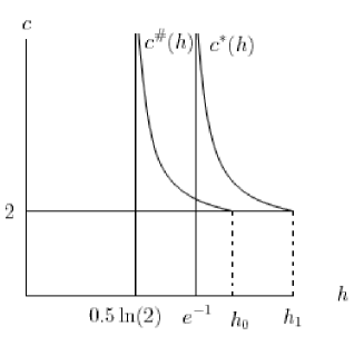
Figure 1: Schematic presentation of the critical speeds and delays.

Theorem 6

Let $u=\varphi(\nu\cdot x+ct),$  $|\nu|=1,$ be a positive monotone traveling front of Eq. (3). Set $\phi(s):=\varphi(cs)$. Then, for some appropriate $t_{0}$, positive $K_{j}$ and every small positive $\sigma$, we have at $t=-\infty$

$$\phi(t+t_{0})=\left\{\begin{array}[]{lll}-K_{2}te^{\lambda t}+O(e^{(2\lambda-\sigma)t}),&\hbox{when}\ c=2,\\ e^{\lambda t}-K_{1}e^{\mu t}+O(e^{(2\lambda-\sigma)t}),&\hbox{when}\,\ 2<c<1.5\sqrt{2},\\ e^{\lambda t}+O(e^{(2\lambda-\sigma)t}),&\hbox{when}\ c\geq 1.5\sqrt{2}=2.121\dots\end{array}\right.$$

Similarly, at $t=+\infty$

$$\phi(t+t_{0})=\left\{\begin{array}[]{llll}1-e^{\lambda_{2}t}+O(e^{(2\lambda_{2}+\sigma)t}),&\hbox{when \ }\ h\leq h_{0},\ c\in[2,c^{\#}(h)]\cap{\mathbb{R}},\\ 1-e^{\lambda_{2}t}+K_{3}e^{\lambda_{1}t}+&\hbox{when }\ h\in(0.5\ln 2,h_{1}]\\ \hskip 14.22636pt+O(e^{(\lambda_{1}-\sigma)t}),&{\hbox{and }c\in(c^{\#}(h),c^{*}(h))},\\ 1-K_{4}te^{\lambda_{2}t}+O(e^{(\lambda_{2}-\sigma)t}),&\hbox{when}\ c=c^{*}(h)\ \hbox{and }h\in(1/e,h_{1}].\end{array}\right.$$

Theorem 6 suggests the way of approximating the traveling front profile: e.g., for $c\not=2,c^{*}(h)$, we can take functions $a_{-}(t):=c_{1}e^{-\lambda t}$ and $a_{+}(t):=1-e^{\lambda_{2}t}$ and glue them together at some point $\tau$. The point $\tau$ and $c_{1}>0$ have to be chosen to assure maximal smoothness of the approximation at $\tau$. As we will see in Section 3, this idea allows to construct reasonable lower approximations to the exact traveling wave. See also Figure 2 below.

Remark 7

As it was showed by Ablowitz and Zeppetella [1], equation (1) has the explicit exact wavefront solution $u=\varphi_{\star}(\nu\cdot x+ct),$  $|\nu|=1,$ with $c=5/\sqrt{6}=2.041\dots$ and the (scaled) profile

$$\phi_{\star}(s)=\left(\frac{1}{2}+\frac{1}{2}\tanh(\frac{5s}{12}+s_{0})\right)^{2},\ \phi_{\star}(s):=\varphi_{\star}(cs).$$

If we select $s_{0}=0.5\ln 2$, then

$$\phi_{\star}(s)=1-2e^{-5s/6-2s_{0}}+O(e^{-5s/4})=1-e^{-5s/6}+O(e^{-5s/4}),\ s\to+\infty,$$

so that $\phi_{\star}=\lim_{j\to+\infty}\mathcal{A}^{j}\phi_{-}$ in view of Theorem 4 and the uniqueness (up to translations) of the traveling front for the non-delayed KPP-Fisher equation. Figure 2 (on the left) shows five approximations $\mathcal{A}^{j}\phi_{-},j=0,1,2,3,4,$ and the exact solution $\phi_{\star}$, the graphs are ordered as $\phi_{-}<\mathcal{A}\phi_{-}<\mathcal{A}^{2}\phi_{-}<\mathcal{A}^{3}\phi_{-}<\phi_{\star}$. On the right, the four first approximations $\mathcal{B}^{j}\phi_{-},j=0,1,2,3,$ of $\phi$ are plotted when $c=2,\ h=0.56$. It should be noted that the limit function $\phi$ and the initial approximation $\phi_{-}$ have the same first two terms $(1-\exp(\lambda_{2}t))$ of their asymptotic expansions at $+\infty$. See Theorem 4 and Sections 3,4. However, as the analysis of the Ablowitz-Zeppetella solution shows, these $\phi$ and $\phi_{-}$ may have different first terms of their expansions at $-\infty$. This partially explains a better agreement between the exact solution and their approximations for $t\geq\tau=0.487\dots$ on the left picture (the value of $\tau$ is given in Section 3).

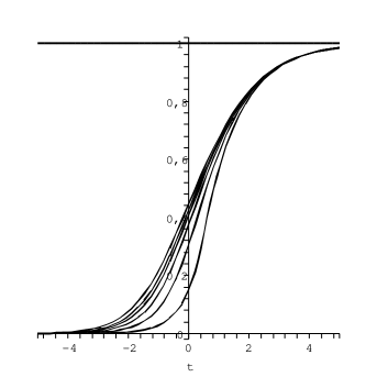
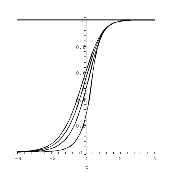
Figure 2: On the left: increasing sequence of approximated waves $\mathcal{A}^{j}\phi_{-},j=0,1,2,3,4,$ and the Ablowitz-Zeppetella exact solution $\phi_{\star}$ ($\epsilon=0.24$ and $h=0$). On the right: approximations $\mathcal{B}^{j}\phi_{-},j=0,1,2,3$ ($\epsilon=0.25$ and $h=0.56$).

The structure of the remainder of this paper is as follows. In Section 2, the characteristic function of the variational equation at the positive steady state is analyzed. In the third [the fourth] section, we present a lower [an upper] solution. Section 5 contains some comments on the smoothness of upper and lower solutions. Theorems 4 and 6 are proved in Sections 6 and 7, respectively.

2 Characteristic equation at the positive steady state

In this section, we study the zeros of $\psi(z,\epsilon):=\epsilon z^{2}-z-\exp(-zh),\ \epsilon,h>0.$ It is straightforward to see that $\psi$ always has a unique positive simple zero. Since $\psi^{\prime\prime\prime}(z,\epsilon)$ is positive, $\psi$ can have at most three (counting multiplicities) real zeros, one of them positive and the other two (when they exist) negative. Lemma 3 in the introduction provides a criterion for the existence of two negative zeros $\lambda_{1}\leq\lambda_{2}<0$. We start by proving this result: [Proof.][Lemma 3] Consider the equation $-z=\exp(-zh).$ An easy analysis shows that (i) this equation has exactly two real simple solutions $z_{1}<z_{2}<0,$ $z_{2}>-e,$ if $h\in(0,1/e)$, (ii) it has one double real root $z_{1}=z_{2}=-e$ if $h=1/e$, and (iii) it does not have any real root if $h>1/e$. As a consequence,

$$\epsilon z^{2}-z=\exp(-zh)$$ (8)

has two negative simple solutions if $\epsilon>0$ and $h\in(0,1/e]$.

A similar argument shows that for every $h>1/e$ there exists $\epsilon^{*}(h)>0$ such that Eq. (8) (a) has two negative simple roots if $\epsilon>\epsilon^{*}(h)$, (b) has one negative double root if $\epsilon=\epsilon^{*}(h)$, (c) does not have any solution if $\epsilon<\epsilon^{*}(h)$. In particular, $\epsilon=\epsilon^{*}(h),z=\lambda_{1}(h)=\lambda_{2}(h),$ solve the system

$$\epsilon z^{2}-z=\exp(-zh),\quad 2\epsilon z-1=-h\exp(-zh),$$

which yields the parametric representation for $\epsilon^{*}(h)$ given in the introduction.

Finally, a direct graphical analysis of (8) shows that $\epsilon^{*}(h)$ is increasing with respect to $h$. Hence, since $\epsilon^{*}(h)\leq 0.25$, we conclude that $h\leq(\epsilon^{*})^{-1}(0.25)=:h_{1}=0.560771\dots$ $\square$

Lemma 8

Let $\lambda_{1}\leq\lambda_{2}<0$ be two negative zeros of $\psi(z,\epsilon)$ and $\epsilon\in(0,0.25]$ be fixed. Then $\lambda_{1}\leq 2\lambda_{2}$ if and only if one of the following conditions holds

1. $0<h\leq 0.5\ln 2=0.347\dots$;

2. $\epsilon\geq\epsilon^{\#}(h)$ and $0.5\ln 2<h\leq\ h_{0}:=0.5336619208\dots$.

[Proof.] This lemma can be proved analogously to the previous one, we briefly outline the main arguments. First, for each fixed positive $\epsilon^{\#}$ we may find $h(\epsilon^{\#})>0$ such that $\lambda_{1}<2\lambda_{2}$ if $h\in(0,h(\epsilon^{\#}))$ and $\lambda_{1}=2\lambda_{2}$ if $h=h(\epsilon^{\#})$. In this way,

$$\epsilon^{\#}\lambda_{2}^{2}-\lambda_{2}=\exp(-\lambda_{2}h(\epsilon^{\#})),\quad 4\epsilon^{\#}\lambda_{2}^{2}-2\lambda_{2}=\exp(-2\lambda_{2}h(\epsilon^{\#})),$$

which yields representation (7). Now, we complete the proof by noting that $h(\epsilon)$ is continuous and strictly increasing on $(0,+\infty)$ and $h(0+)=0.5\ln 2,\ h_{0}=h(0.25)$. $\square$

Lemma 9

Let $\lambda_{1}\leq\lambda_{2}<0$ be two negative zeros of $\psi(z,\epsilon)$ and $\epsilon\in(0,0.25]$ be fixed. Then $\Re\lambda_{j}<\lambda_{1}$ for every complex root of $\psi(z,\epsilon)=0$.

[Proof.] Set $\alpha:=(1+2\epsilon-\sqrt{1+4\epsilon^{2}})/(2\epsilon),\ a:=-e^{-\alpha h}/(\sqrt{1+4\epsilon^{2}}-2\epsilon),\ k:=\epsilon/(\sqrt{1+4\epsilon^{2}}-2\epsilon)$. Then $\alpha,k>0,a<0,$ and

$$\psi(z+\alpha)=(\sqrt{1+4\epsilon^{2}}-2\epsilon)(kz^{2}-z-1+ae^{-zh}).$$

It is easy to see that $p(z):=kz^{2}-z-1+ae^{-zh}$ also has two negative and one positive root. Since the translation $z\to z+\alpha$ of the complex plain does not change the mutual position of zeros of $\psi$, the statement of Lemma 9 follows now from [31, Remarks 19,20]. $\square$

3 A lower solution when $\lambda_{1}<\lambda_{2}$

In this section, we assume either condition (1) or condition (2) of Theorem 4 holds. In addition, let $c\in[2,c^{*}(h))$ so that $\lambda_{1}<\lambda_{2}$ (where $\lambda_{1}:=-\infty$ if $h=0$) and $\lambda\leq\mu$. Set

$$\tau=\frac{1}{\lambda_{2}}\ln\frac{\lambda}{\lambda-\lambda_{2}}>0,\quad\phi_{-}(t)=\left\{\begin{array}[]{ll}{\frac{-\lambda_{2}}{\lambda-\lambda_{2}}e^{\lambda(t-\tau)}},&\hbox{if}\ t\leq\tau,\vspace{5mm}\\ 1-e^{\lambda_{2}t}&\hbox{if}\ t\geq\tau.\end{array}\right.$$

It is easy to see that $\phi_{-}\in C^{1}(\mathbb{R})\cap C^{2}(\mathbb{R}\setminus\{\tau\})$ with $\phi_{-}^{\prime}(t)>0,\ t\in\mathbb{R}$, and

$$\epsilon\phi_{-}^{\prime\prime}(t)-\phi_{-}^{\prime}(t)+\phi_{-}(t)(1-\phi_{-}(t-h))<0,\quad t\in{\mathbb{R}}\setminus(\tau,\tau+h].$$ (9)

Lemma 10

Inequality (9) holds for all $t\in{\mathbb{R}}$.

[Proof.] The case $h=0$ is obvious, so let $h>0$. It suffices to consider $t\in(\tau,\tau+h]$. If we take $t\in(\tau,\tau+h]$, then

$$\epsilon\phi_{-}^{\prime\prime}(t)-\phi_{-}^{\prime}(t)+\phi_{-}(t)(1-\phi_{-}(t-h))=-\epsilon\lambda_{2}^{2}e^{\lambda_{2}t}+\lambda_{2}e^{\lambda_{2}t}+$$

$$(1-e^{\lambda_{2}t})(1+\frac{\lambda_{2}}{\lambda-\lambda_{2}}e^{\lambda(t-\tau-h)})=-e^{\lambda_{2}(t-h)}+(1-e^{\lambda_{2}t})(1+\frac{\lambda_{2}}{\lambda-\lambda_{2}}e^{\lambda(t-\tau-h)})=$$

$$1-e^{\lambda_{2}(t-h)}+\frac{\lambda_{2}}{\lambda-\lambda_{2}}e^{\lambda(t-\tau-h)}-e^{\lambda_{2}t}-e^{\lambda_{2}t}\frac{\lambda_{2}}{\lambda-\lambda_{2}}e^{\lambda(t-\tau-h)}=$$

$$1+\frac{\lambda_{2}}{\lambda-\lambda_{2}}e^{\lambda s}-\frac{\lambda}{\lambda-\lambda_{2}}e^{\lambda_{2}s}-\frac{\lambda}{\lambda-\lambda_{2}}e^{\lambda_{2}(s+h)}-\frac{\lambda\lambda_{2}}{(\lambda-\lambda_{2})^{2}}e^{\lambda_{2}(s+h)}e^{\lambda s}=:\rho(s)$$

where $s=t-\tau-h\in(-h,0]$. The direct differentiation shows that

$$\rho^{\prime}(s)=\frac{-\lambda_{2}\lambda}{\lambda-\lambda_{2}}\left[-e^{\lambda s}+e^{\lambda_{2}s}+e^{\lambda_{2}(s+h)}(1+\frac{\lambda+\lambda_{2}}{\lambda-\lambda_{2}}e^{\lambda s})\right]>0,$$

$${\rm since}\ e^{\lambda s}\leq 1,\ e^{\lambda_{2}s}\geq 1,\ {\rm and}\ (1+\frac{\lambda+\lambda_{2}}{\lambda-\lambda_{2}}e^{\lambda s})>1,{\rm if}\ \lambda+\lambda_{2}\geq 0,$$

$$(1+\frac{\lambda+\lambda_{2}}{\lambda-\lambda_{2}}e^{\lambda s})\geq 1+\frac{\lambda+\lambda_{2}}{\lambda-\lambda_{2}}=\frac{2\lambda}{\lambda-\lambda_{2}}>0,{\rm if}\ \lambda+\lambda_{2}<0.$$

Finally, we have that $\rho(s)<0$ for all $s\in[-h,0]$ since $\rho^{\prime}(s)>0$ and

$$\rho(0)=-\lambda^{2}(\lambda-\lambda_{2})^{-2}e^{\lambda_{2}h}<0.\hskip 142.26378pt\square$$

Remark 11 (A lower solution when $\lambda_{1}=\lambda_{2}$)

We can not use $\phi_{-}$ as a lower solution when $c=c^{*}(h),\ 1/e<h\leq\ h_{1}$. Indeed, by Theorem 6, in this case $\phi_{-}$ converges to the positive steady state faster than the heteroclinic solutions. In Section 5, we will present an adequate lower solution for this situation. However, it will not be $C^{1}$-smooth.

4 An upper solution when $\lambda_{1}<\lambda_{2}$

Suppose that $\lambda_{1}<\lambda_{2}$ and set $\phi_{2}(t):=1-e^{\lambda_{2}t}+e^{rt}$ for some $r\in(\lambda_{1},\lambda_{2})$. Recall that $\lambda_{1}:=-\infty$ if $h=0$. Obviously, $\psi(r,\epsilon)>0$ and $\phi_{2}(t)\in(0,1)$ for $t>0$. Next, it is immediate to check that $\phi_{2}:{\mathbb{R}}\to{\mathbb{R}}$ has a unique critical point (absolute minimum) $t_{0}=t_{0}(r)>0$:

$$t_{0}(r)=\frac{\ln(-r)-\ln(-\lambda_{2})}{\lambda_{2}-r},\quad\lambda_{2}e^{\lambda_{2}t_{0}}=re^{rt_{0}}.$$

Observe that if $h\in(0,1/e)$, then we can assume that $t_{0}(r)\geq h$ since

$$\lim_{r\to\lambda_{2}-}t_{0}(r)=-1/\lambda_{2}>1/e>h,$$

where the last inequalities were established in the proof of Lemma 3. It is clear that the function

$$\phi_{+}(t)=\left\{\begin{array}[]{ll}\phi_{2}(t),&\hbox{if}\ t\geq t_{0}(r),\\ \phi_{2}(t_{0}(r)),&\hbox{if}\ t\leq t_{0}(r)\end{array}\right.$$

is $C^{1}$-continuous and increasing on ${\mathbb{R}}$. Moreover, $\phi_{+}(t)\in C^{2}({\mathbb{R}}\setminus\{t_{0}(r)\})$.

Lemma 12

For all $r<\lambda_{2}$ sufficiently close to $\lambda_{2}$, $\phi_{+}$ satisfies the inequality

$$\epsilon\phi^{\prime\prime}(t)-\phi^{\prime}(t)+\phi(t)(1-\phi(t-h))\geq 0,\quad t\in{\mathbb{R}}.$$

[Proof.] Step I. First we prove that, for all $t\geq t_{0}$, the following inequality holds:

$$(\mathfrak{N}\phi_{2})(t):=\epsilon\phi^{\prime\prime}_{2}(t)-\phi^{\prime}_{2}(t)+\phi_{2}(t)(1-\phi_{2}(t-h))\geq 0.$$

In particular, this implies that $(\mathfrak{N}\phi_{+})(t)\geq 0$ if $t\geq t_{0}+h$. For $t=t_{0}+s$, we have that

$$(\mathfrak{N}\phi_{2})(t)=\psi(r,\epsilon)e^{rt}-\psi(\lambda_{2},\epsilon)e^{\lambda_{2}t}+(-e^{\lambda_{2}t}+e^{rt})(e^{\lambda_{2}(t-h)}-e^{r(t-h)})=$$

$$\psi(r,\epsilon)e^{rt}+(-e^{\lambda_{2}t}+e^{rt})(e^{\lambda_{2}(t-h)}-e^{r(t-h)})=$$

$$e^{rt_{0}}\left[\psi(r,\epsilon)e^{rs}+(-\frac{r}{\lambda_{2}}e^{\lambda_{2}s}+e^{rs})e^{rt_{0}}(\frac{r}{\lambda_{2}}e^{\lambda_{2}(s-h)}-e^{r(s-h)})\right]=$$

$$e^{r(t_{0}+s)}\left[\psi(r,\epsilon)+(-\frac{r}{\lambda_{2}}e^{(\lambda_{2}-0.5r)s}+e^{0.5rs})e^{rt_{0}}(\frac{r}{\lambda_{2}}e^{-\lambda_{2}h}e^{(\lambda_{2}-0.5r)s}-e^{-rh}e^{0.5rs})\right]=$$

$$e^{rt}\left[\psi(r,\epsilon)+A_{1}(s)e^{rt_{0}}A_{2}(s)\right].$$

It is easy to see that $A_{j}(+\infty)=0$ and that $A_{j}$ has a unique critical point $s_{j}$, with

$$\lim_{r\to\lambda_{2}-}s_{1}(r)=-1/\lambda_{2},\lim_{r\to\lambda_{2}-}s_{2}(r)=h-1/\lambda_{2}.$$

Therefore, for some small $\delta>0$ and for all $r$ close to $\lambda_{2}$, the function $A_{1}(s)e^{rt_{0}}A_{2}(s)$ is strictly increasing to $0$ on the interval $[h-1/\lambda_{2}+\delta,+\infty)$ and it is strictly decreasing on $[0,-1/\lambda_{2}-\delta]$. This means that if $(\mathfrak{N}\phi_{2})(t)\geq 0$ for all $t\in[t_{0}-1/\lambda_{2}-\delta,t_{0}+h-1/\lambda_{2}+\delta]$ then $(\mathfrak{N}\phi_{2})(t)\geq 0$ for $t\geq t_{0}$. In order to prove the former, consider the expression

$$\frac{e^{-rt_{0}}}{r-\lambda_{2}}\left(\epsilon\phi^{\prime\prime}_{2}(t)-\phi^{\prime}_{2}(t)+\phi_{2}(t)(1-\phi_{2}(t-h))\right)=$$

$$\frac{\psi(r,\epsilon)e^{rs}+(-\frac{r}{\lambda_{2}}e^{\lambda_{2}s}+e^{rs})e^{rt_{0}}(\frac{r}{\lambda_{2}}e^{\lambda_{2}(s-h)}-e^{r(s-h)})}{r-\lambda_{2}}:=\Gamma_{\epsilon}(r,s).$$

Since $\Gamma_{\epsilon}(r,s)$ is analytical on some open neighborhood $\Omega\subset{\mathbb{R}}^{2}$ of the compact segment $\{\lambda_{2}\}\times[-1/\lambda_{2}-\delta,h-1/\lambda_{2}+\delta]\subset{\mathbb{R}}^{2}$, we find that, for every fixed $\epsilon>0$,

$$\lim_{r\to\lambda_{2}-}\Gamma_{\epsilon}(r,s)=\psi^{\prime}(\lambda_{2},\epsilon)e^{\lambda_{2}s}<0$$

uniformly on $[-1/\lambda_{2}-\delta,h-1/\lambda_{2}+\delta]$. As a consequence, we obtain that

$$\epsilon\phi^{\prime\prime}_{2}(t)-\phi^{\prime}_{2}(t)+\phi_{2}(t)(1-\phi_{2}(t-h))>0,\quad t\in[t_{0}-1/\lambda_{2}-\delta,t_{0}+h-1/\lambda_{2}+\delta].$$

Step II. Now, we are ready to prove that $(\mathfrak{N}\phi_{+})(t)\geq 0,\ t\in[t_{0},t_{0}+h].$ Indeed, since $\phi_{2}(t_{0})\leq\phi_{2}(t-h)$ for $t\in[t_{0},t_{0}+h]$, we have that

$$(\mathfrak{N}\phi_{+})(t)=\epsilon\phi_{2}^{\prime\prime}(t)-\phi_{2}^{\prime}(t)+\phi_{2}(t)(1-\phi_{2}(t_{0}))\geq$$

$$\phi_{2}^{\prime\prime}(t)-\phi_{2}^{\prime}(t)+\phi_{2}(t)(1-\phi_{2}(t-h))\geq 0,\quad t\in[t_{0},t_{0}+h].$$

Finally, since the inequality $(\mathfrak{N}\phi_{+})(t)>0,\ t\leq t_{0}$, is obvious, the proof of the lemma is completed. $\square$

Remark 13 (An upper solution when $\lambda_{1}=\lambda_{2}$)

We can not use $\phi_{+}$ as an upper solution when $c=c^{*}(h),\ 1/e<h\leq\ h_{1}$. Moreover, in this case it is not difficult to show that $\phi_{+}$ satisfies inequality (9) for all $r<\lambda_{2}$ sufficiently close to $\lambda_{2}$ and for large positive $t$.

5 Some comments on upper and lower solutions

5.1 Non-smooth solutions

The problem of smoothness of the lower (upper) solutions is an interesting and important aspect of the topic, see [5, 23]. As we have seen in the previous sections, $C^{1}-$smoothness condition can be rather restrictive even when a simple nonlinearity (the birth function) is considered. The above mentioned works [23] show that continuous and piece-wise $C^{1}-$continuous lower (upper) solutions $\phi_{\pm}$ still can be used if some sign conditions are fulfilled at the points of discontinuity of $\phi_{\pm}^{\prime}$. Moreover, as we prove it below even discontinuous functions $\phi_{\pm}$ can be also used. We start with a simple result of the theory of impulsive systems [29] which can be viewed as a version of the Perron theorem for piece-wise continuous solutions, cf. [5].

Lemma 14

Let $\psi:{\mathbb{R}}\to{\mathbb{R}}$ be a bounded classical solution of the second order impulsive equation

$$\psi^{\prime\prime}+a\psi^{\prime}+b\psi=f(t),\quad\Delta\psi|_{t_{j}}=\alpha_{j},\quad\Delta\psi^{\prime}|_{t_{j}}=\beta_{j},$$

where $\{t_{j}\}$ is a finite increasing sequence, $f:{\mathbb{R}}\to{\mathbb{R}}$ is bounded and continuous at every $t\not=t_{j}$ and the operator $\Delta$ is defined by $\Delta w|_{t_{j}}:=w(t_{j}+)-w(t_{j}-)$. Assume that $z^{2}+az+b=0$ has two positive roots $0<\lambda\leq\mu$. Then

$${\rm\ if}\ \lambda<\mu\ {\rm\ we\ have\ that}\ \psi(t)=\frac{1}{\mu-\lambda}\int_{t}^{+\infty}\left(e^{\lambda(t-s)}-e^{\mu(t-s)}\right)f(s)ds$$ (10)

$$+\frac{1}{\mu-\lambda}\sum_{t<t_{j}}\left[\left(\lambda e^{\mu(t-t_{j})}-\mu e^{\lambda(t-t_{j})}\right)\alpha_{j}+\left(e^{\lambda(t-t_{j})}-e^{\mu(t-t_{j})}\right)\beta_{j}\right],\ \ t\not=t_{j};$$

$${\rm\ if}\ \lambda=\mu=-0.5a\ {\rm\ we\ have\ that}\ \psi(t)=\int_{t}^{+\infty}(s-t)e^{-0.5a(t-s)}f(s)ds+$$

$$\sum_{t<t_{j}}e^{-0.5a(t-t_{j})}\left[(t_{j}-t)(\beta_{j}+0.5a\alpha_{j})-\alpha_{j}\right],\ \ t\not=t_{j}.$$

[Proof.] See [29, Theorem 87]. $\square$ Next, the corollary below shows that our lower solution is an upper solution in the sense of Wu and Zou [35]:

Corollary 15

Assume that $\psi:{\mathbb{R}}\to{\mathbb{R}}$ is bounded and such that the derivatives $\psi^{\prime},\psi^{\prime\prime}:{\mathbb{R}}\setminus\{t_{j}\}\to{\mathbb{R}}$ exist and are bounded. Suppose also that $\psi$ is a classical solution of the impulsive inequality

$$\psi^{\prime\prime}+a\psi^{\prime}+b\psi\leq f(t),\quad\Delta\psi|_{t_{j}}=\alpha_{j},\quad\Delta\psi^{\prime}|_{t_{j}}=\beta_{j}.$$

If $\alpha_{j}\geq 0,\ \beta_{j}\leq 0$, then

$$\psi(t)\leq\frac{1}{\mu-\lambda}\int_{t}^{+\infty}\left(e^{\lambda(t-s)}-e^{\mu(t-s)}\right)f(s)ds,\quad{\rm when}\ \lambda<\mu,$$

$$\psi(t)\leq\int_{t}^{+\infty}(s-t)e^{-0.5a(t-s)}f(s)ds,\quad{\rm when}\ \lambda=\mu=-0.5a.$$

[Proof.] Suppose that $\lambda<\mu$, the case $\lambda=\mu$ is similar. Clearly, $q(t):=f(t)-(\psi^{\prime\prime}(t)+a\psi^{\prime}(t)+b\psi(t))\geq 0$ and $\lambda e^{\mu(t-t_{j})}<\mu e^{\lambda(t-t_{j})},$ $\ e^{\lambda(t-t_{j})}>e^{\mu(t-t_{j})}$ for $t<t_{j}$. Thus the desired inequality follows from (10). $\square$

5.2 A lower solution when $\lambda_{1}=\lambda_{2},\ h\in(1/e,h_{1}]$

In Section 3, a lower $C^{1}-$ solution was presented for the case when $\lambda_{1}<\lambda_{2}$. However, to apply our iterative procedure in the critical case $\lambda_{1}=\lambda_{2}$, we also need to construct a lower solution for the corresponding range of parameters. It is worth to mention that our approach does not require any upper solution once a lower solution is found and the existence of the heteroclinic is proved, see Corollary 26. Here, we provide a continuous and piece-wise analytic lower solution $\phi_{-}(t)$ if $\lambda_{1}=\lambda_{2}$. Our solution has a unique singular point $\tau^{\prime}$ where $\Delta\phi_{-}|_{\tau^{\prime}}=0,\quad\Delta\phi_{-}^{\prime}|_{\tau^{\prime}}>0$. This shows that, in general, the sign conditions of Corollary 15 need not to be satisfied.

Take some positive $A>(e^{-\lambda_{2}h}-1)/h$ and let $\tau^{\prime}$ be the positive root of the equation $At+1=e^{-\lambda_{2}t}$. It is easy to see that $\tau^{\prime}>h$. Consider the piece-wise smooth function $\phi_{-}:{\mathbb{R}}\to[0,1)$ defined by

$$\phi_{-}(t)=\left\{\begin{array}[]{ll}0,&\hbox{if}\ t\leq\tau^{\prime},\\ 1-(At+1)e^{\lambda_{2}t},&\hbox{if}\ t\geq\tau^{\prime}.\end{array}\right.$$ (11)

Proposition 16

The inequality $(\mathcal{K}\phi_{-})(t)>\phi_{-}(t)$ holds for all $t\in{\mathbb{R}}$.

[Proof.] Below, we are assuming that $h\not=h_{1}$ so that $\lambda<\mu$ and $\mathcal{K}=\mathcal{A}$; however, a similar argument works also in the case $h=h_{1}$ (when $\mathcal{K}=\mathcal{B}$). It suffices to prove that $(\mathcal{A}\phi_{-})(t)>\phi_{-}(t)$ for $t\geq\tau^{\prime}$. Let $C^{2}-$ smooth function $\psi$ be defined by

$$\psi(t)=\left\{\begin{array}[]{lll}1-(At+1)e^{\lambda_{2}t},&\hbox{if}\ t\geq\tau^{\prime}-h,\\ B(t),&\hbox{if}\ 0\leq t\leq\tau^{\prime}-h,\\ 0,&\hbox{if}\ t\leq 0,\end{array}\right.$$

for some appropriate continuous decreasing $B(t)$. Set

$$\zeta(t):=\epsilon\psi^{\prime\prime}(t)-\psi^{\prime}(t)+\psi(t)(1-\psi(t-h)).$$

It is easy to check that $\zeta\in C({\mathbb{R}},{\mathbb{R}})$ is bounded on ${\mathbb{R}}$ and $\zeta(t)<0$ for all $t>\tau^{\prime}$. But then, for all $t>\tau^{\prime}$, we have that

$$\phi_{-}(t)=\psi(t)=(\mathcal{A}\psi)(t)+\frac{1}{\epsilon(\mu-\lambda)}\int_{t}^{+\infty}\left(e^{\lambda(t-s)}-e^{\mu(t-s)}\right)\zeta(s)ds<(\mathcal{A}\psi)(t)\leq$$

$$=\frac{1}{\epsilon(\mu-\lambda)}\int_{t}^{+\infty}(e^{\lambda(t-s)}-e^{\mu(t-s)})\phi_{-}(s)\phi_{-}(s-h)ds=(\mathcal{A}\phi_{-})(t).\quad\square$$

5.3 Ordering the upper and lower solutions

Finally, we show that the condition of the correct ordering $\phi_{-}\leq\phi_{+}$ is not at all restrictive provided that solutions $\phi_{\pm}$ are monotone and satisfy some natural asymptotic relations.

Lemma 17

Assume that functions $\phi_{\pm}:{\mathbb{R}}\to[0,1),$ $j=1,2,$ are increasing and, for some fixed $k\in\{0,1\}$, the following holds

$$\lim_{t\to-\infty}\phi_{\pm}(t)e^{-\lambda t}=\alpha_{\pm},\ \lim_{t\to+\infty}(1-\phi_{\pm}(t))t^{-k}e^{-\lambda_{2}t}=\beta_{\pm,k},$$

where $\beta_{\pm,k}>0$, and $\alpha_{-}\in[0,+\infty)$, $\alpha_{+}\in(0,+\infty]$. Then there exists a real number $\sigma$ such that $\phi_{-}(t)<\phi_{+}(t+\sigma)$ for all $t\in{\mathbb{R}}$.

[Proof.] It is clear that $\phi_{-}(-\infty)=0$ and $\phi_{\pm}(+\infty)=1$. Let $\sigma_{0}$ be sufficiently large to satisfy $\beta_{+,k}e^{\lambda_{2}\sigma_{0}}<\beta_{-,k},\ \alpha_{-}e^{-\lambda\sigma_{0}}<\alpha_{+}$ . Then there exist $t_{1},t_{2}$ such that $t_{1}<t_{2}$ and $\phi_{-}(t-\sigma_{0})<\phi_{+}(t),\ t\in\mathcal{I}:=(-\infty,t_{1}]\cup[t_{2},+\infty)$. Now, set $\sigma=\sigma_{0}+(t_{2}-t_{1})$. Since both functions are increasing, we have

$$\phi_{-}(t-\sigma)\leq\phi_{-}(t-\sigma_{0})<\phi_{+}(t),\quad t\in\mathcal{I},$$

$$\phi_{-}(t-\sigma)<\phi_{+}(t-(t_{2}-t_{1}))\leq\phi_{+}(t),\quad t\in[t_{1},t_{2}].\qquad\square$$

6 Proof of Theorem 4

6.1. Necessity. Let $u(t,x)=\zeta(ct+\nu\cdot x)$ be a positive bounded monotone solution of the delayed KPP-Fisher equation. Then $\varphi(t)=\zeta(ct)$ satisfies

$$\epsilon\varphi^{\prime\prime}(t)-\varphi^{\prime}(t)+\varphi(t)(1-\varphi(t-h))=0,\quad t\in{\mathbb{R}},$$ (12)

$$\epsilon\varphi^{\prime}(t)=\epsilon\varphi^{\prime}(0)-\varphi(0)+\varphi(t)+\int_{0}^{t}\varphi(s)(1-\varphi(s-h))ds.$$

The latter relation implies that $\varphi(\pm\infty)\in\{0,1\}$ since otherwise $\varphi^{\prime}(\pm\infty)=\infty$. Hence $\varphi:{\mathbb{R}}\to(0,1)$. Let $\phi\in C^{2}({\mathbb{R}},(0,1))$ be an arbitrary solution of (12). Suppose for a moment that $\phi^{\prime}(t_{0})=0$. Then necessarily $\phi^{\prime\prime}(t_{0})<0$ so that $t_{0}$ is the unique critical point (absolute maximum) of $\phi$. But then $\phi^{\prime}(s)<0$ for $s>t_{0}$, so that $\phi^{\prime\prime}(s)<0,\ s\geq t_{0}$, which yields the contradiction $\phi(+\infty)=-\infty$. In consequence, either $\phi^{\prime}(s)>0$ or $\phi^{\prime}(s)<0$ for all $s\in{\mathbb{R}}$. But as we have seen, $\phi^{\prime}(s)<0$ implies $\phi(+\infty)=-\infty$, a contradiction. Hence, any solution $\phi\in C^{2}({\mathbb{R}},(0,1))$ of (12) satisfies $\phi^{\prime}(t)>0,\ \phi(-\infty)=0,\ \phi(+\infty)=1$.

Lemma 18

If $\phi\in C^{2}({\mathbb{R}},(0,1))$ satisfies (12), then $\epsilon\in(0,0.25]$.

[Proof.] Suppose for a moment that $\epsilon>0.25$. Then the characteristic equation $\epsilon\lambda^{2}-\lambda+1=0$ associated with the trivial steady state of (12) has two simple complex conjugate roots $\omega_{\pm}=(2\epsilon)^{-1}(1\pm i\sqrt{4\epsilon-1})$.

Since $\phi\in C^{2}({\mathbb{R}},(0,1))$ is a solution of (12), it holds that $\phi^{\prime}(t)>0,\ t\in{\mathbb{R}},$ $\ \phi(-\infty)=0$. Set $z(t)=(\phi(t),\phi^{\prime}(t))^{T}$, it is easy to check that $z(t)$ satisfies the following asymptotically autonomous linear differential equation

$$z^{\prime}(t)=(A+R(t))z(t),\ t\in{\mathbb{R}},\quad A=\left(\begin{array}[]{cc}0&1\\ -1/\epsilon&1/\epsilon\\ \end{array}\right),\ R(t)=\left(\begin{array}[]{cc}0&0\\ \phi(t-h)/\epsilon&0\\ \end{array}\right).$$

Since $R(-\infty)=0,\ \int_{-\infty}^{0}|R^{\prime}(t)|dt=\phi(-h)$ and the eigenvalues $\omega_{\pm}$ of $A$ are complex conjugate, we can apply the Levinson theorem [10, Theorem 1.8.3] to obtain the following asymptotic formulas at $t=-\infty$:

$$\phi(t)=(a+o(1))e^{t/(2\epsilon)}\cos(t\sqrt{4\epsilon-1}(1+o(1))+b+o(1)),$$

$$\phi^{\prime}(t)=(c+o(1))e^{t/(2\epsilon)}\sin(t\sqrt{4\epsilon-1}(1+o(1))+d+o(1)),$$

where $a^{2}+c^{2}\not=0$. But this means that either $\phi(t)$ or $\phi^{\prime}(t)$ is oscillating around zero, a contradiction. $\square$

Lemma 19

If $h>h_{1}$ or $h\in(1/e,h_{1}]$ and $c>c^{*}(h)$ then Eq. (12) does not have any solution $\phi\in C^{2}({\mathbb{R}},(0,1))$.

[Proof.] On the contrary, let us assume that Eq. (12) has a solution $\phi\in C^{2}({\mathbb{R}},(0,1))$. Then Lemma 18 implies that $\epsilon\in(0,0.25]$ and therefore the assumptions of this lemma imply that $\psi(z,\epsilon)$ does not have negative zeros. Following the approach in [32], we will show that this will force $\phi(t)$ to oscillate about the positive equilibrium. For the convenience of the reader, the proof is divided in several steps.

Claim I: $y(t):=1-\phi(t)>0$ has at least exponential decay as $t\to+\infty$. First, observe that

$$\epsilon y^{\prime\prime}(t)-y^{\prime}(t)=\phi(t)y(t-h),\quad t\in{\mathbb{R}}.$$ (13)

Therefore, with $\gamma:=\phi(t_{0})$, which is close to $1$, and $g(t):=\phi(t)y(t-h)-\phi(t_{0})y(t)$, we obtain that

$$\epsilon y^{\prime\prime}(t)-y^{\prime}(t)-\gamma y(t)-g(t)=0,\ t\in{\mathbb{R}}.$$

Note that $g(t)>0$ for all sufficiently large $t$. Since $y(t),g(t)$ are bounded on ${\mathbb{R}}$, it holds that

$$y(t)=-\frac{1}{\epsilon(m-l)}\left(\ \int_{-\infty}^{t}e^{l(t-s)}g(s)ds+\int_{t}^{+\infty}e^{m(t-s)}g(s)ds\right),$$

where $l<0$ and $0<m$ are roots of $\epsilon z^{2}-z-\gamma=0$. The latter representation of $y(t)$ implies that there exists $T_{0}$ such that

$$y^{\prime}(t)-ly(t)=-\frac{1}{\epsilon}\int_{t}^{+\infty}e^{m(t-s)}g(s)ds<0,\ t\geq T_{0}.$$ (14)

Hence, $(y(t)\exp(-lt))^{\prime}<0,\ t\geq T_{0},$ and therefore

$$y(t)\leq y(s)e^{l(t-s)},\quad t\geq s\geq T_{0},\quad g(t)=O(e^{lt}),\ t\to+\infty.$$ (15)

It is easy to see that these estimates are valid for every negative $l>(2\epsilon)^{-1}(1-\sqrt{1+4\epsilon})$. Finally, (14), (15) imply that $y^{\prime}(t)=O(e^{lt}),\ t\to+\infty$.

Claim II: $y(t):=1-\phi(t)>0$ is not superexponentially small as $t\to+\infty$.
We already have proved that $y(t)$ is strictly decreasing and positive on ${\mathbb{R}}$. Since the right hand side of Eq. (13) is positive and integrable on ${\mathbb{R}}_{+}$, and since $y(t)$ is a bounded solution of (13) satisfying $y(+\infty)=0$, we find that

$$y(t)=\int_{t}^{+\infty}(1-e^{(t-s)/\epsilon})\phi(s)y(s-h)ds.$$ (16)

As a consequence, there exists $T_{1}$ such that

$$y(t)\geq 0.5(1-e^{-0.5h/\epsilon})\int_{t-0.5h}^{t}y(s)ds:=\xi\int_{t-0.5h}^{t}y(s)ds,\quad t\geq T_{1}-h.$$

Now, since $y(t)>0$ for all $t$, we can find positive $C,\rho$ such that $y(s)>Ce^{-\rho s}$ for all $s\in[T_{1}-h,T_{1}]$. We can assume that $\rho$ is large enough to satisfy the inequality $\xi(e^{0.5\rho h}-1)>{\rho}$. Then we claim that $y(s)>Ce^{-\rho s}$ for all $s\geq T_{1}-h$. Conversely, suppose that $t^{\prime}>T_{1}$ is the leftmost point where $y(t^{\prime})=Ce^{-\rho t^{\prime}}$. Then we get a contradiction:

$$y(t^{\prime})\geq\xi\int_{t^{\prime}-0.5h}^{t^{\prime}}y(s)ds>C\xi\int_{t^{\prime}-0.5h}^{t^{\prime}}e^{-\rho s}ds=Ce^{-\rho t^{\prime}}\xi\frac{e^{0.5\rho h}-1}{\rho}>Ce^{-\rho t^{\prime}}.$$

Claim III: $y(t)>0$ can not hold when $\psi(z,\epsilon)$ does not have any zero in $(-\infty,0)$. Observe that $y(t)=1-\phi(t)$ satisfies

$$\epsilon y^{\prime\prime}(t)-y^{\prime}(t)-(1-y(t))y(t-h)=0,\ t\in{\mathbb{R}},\$$

where in virtue of Claim I, it holds that $(y(t),y^{\prime}(t))=O(lt)$ at $t=+\infty$. Then [25, Proposition 7.2] implies that there exists $\gamma<l$ such that $y(t)=v(t)+O(\exp(\gamma t)),$ $t\to+\infty,$ where $v$ is a non empty (due to Claim II) finite sum of eigensolutions of the limiting equation

$$\epsilon y^{\prime\prime}(t)-y^{\prime}(t)-y(t-h)=0,\ t\in{\mathbb{R}},\$$

associated to the eigenvalues $\lambda_{j}\in F=\{\gamma<\Re\lambda_{j}\leq l\}$. Now, since the set $F$ does not contain any real eigenvalue by our assumption, we conclude that $y(t)$ should be oscillating on $\mathbb{R}_{+}$, a contradiction. $\square$

6.2. Sufficiency. Suppose that $\epsilon\in(0,0.25]$ and let $0<\lambda\leq\mu$ be the roots of the equation $\epsilon z^{2}-z+1=0$. In Lemmas 20-23 below, $\mathcal{K}$ stands either for $\mathcal{A}$ or $\mathcal{B}$ (defined by (5), (6)).

Lemma 20

If $\phi,\psi\in C({\mathbb{R}},(0,1))$ and $\phi(t)\leq\psi(t)$ for all $t\in{\mathbb{R}}$, then $\mathcal{K}\phi,\mathcal{K}\psi\in C({\mathbb{R}},(0,1))$ and $(\mathcal{K}\phi)(t)\leq(\mathcal{K}\psi)(t),\ t\in{\mathbb{R}}$. Moreover, if $\phi$ is increasing then $\mathcal{K}\phi$ is also increasing.

[Proof.] The proof is straightforward. $\square$

Lemma 21

Let $\epsilon\in(0,0.25]$. If $\phi_{+}\in C^{1}({\mathbb{R}},(0,1))$ satisfies the inequality

$$\epsilon\phi^{\prime\prime}(t)-\phi^{\prime}(t)+\phi(t)(1-\phi(t-h))\geq 0$$

for all $t\in{\mathbb{R}}^{\prime}:={\mathbb{R}}\setminus\{T_{1},\dots,T_{m}\}$ and $\phi_{+}^{\prime\prime}(t),\phi_{+}^{\prime}(t)$ are bounded on ${\mathbb{R}}^{\prime}$, then $(\mathcal{K}\phi_{+})(t)\leq\phi_{+}(t)$ for all $t\in{\mathbb{R}}$.

[Proof.] If $\omega(T_{i}):=0$ and

$$\omega(t):=\epsilon\phi_{+}^{\prime\prime}(t)-\phi_{+}^{\prime}(t)+\phi_{+}(t)(1-\phi_{+}(t-h)),\quad t\in{\mathbb{R}}^{\prime}={\mathbb{R}}\setminus\{T_{1},\dots,T_{m}\}$$

then $\omega(t)\geq 0$ for all $t\in{\mathbb{R}}^{\prime},$ $\omega(t)$ is bounded on ${\mathbb{R}}^{\prime}$ and

$$\epsilon\phi_{+}^{\prime\prime}(t)-\phi_{+}^{\prime}(t)+\phi_{+}(t)=\omega_{1}(t),\quad t\in{\mathbb{R}}^{\prime},$$

where $\omega_{1}(t):=\omega(t)+\phi_{+}(t)\phi_{+}(t-h)$ is bounded on ${\mathbb{R}}^{\prime}$. Let now $\epsilon\in(0,0.25)$. By Lemma 14, we obtain that

$$\phi_{+}(t) = \frac{1}{\epsilon(\mu-\lambda)}\int_{t}^{+\infty}\left(e^{\lambda(t-s)}-e^{\mu(t-s)}\right)\omega_{1}(s)ds=$$

$$(\mathcal{A}\phi_{+})(t)+\frac{1}{\epsilon(\mu-\lambda)}\int_{t}^{+\infty}\left(e^{\lambda(t-s)}-e^{\mu(t-s)}\right)\omega(s)ds\geq(\mathcal{A}\phi_{+})(t).$$

The case $\epsilon=0.25$ (which corresponds to $\mathcal{K}=\mathcal{B}$) is completely analogous to the previous one. $\square$ The proof of the next lemma is similar to that of Lemma 21:

Lemma 22

Let $\epsilon\in(0,0.25]$. If $\phi_{-}\in C^{1}({\mathbb{R}},(0,1))$ satisfies the inequality

$$\epsilon\phi^{\prime\prime}(t)-\phi^{\prime}(t)+\phi(t)(1-\phi(t-h))\leq 0$$

for all $t\in{\mathbb{R}}\setminus\{T_{1},\dots,T_{m}\}$ and $\phi_{-}^{\prime\prime}(t),\phi_{-}^{\prime}(t)$ are bounded on ${\mathbb{R}}\setminus\{T_{1},\dots,T_{m}\}$, then $(\mathcal{K}\phi_{-})(t)\geq\phi_{-}(t)$ for all $t\in{\mathbb{R}}$.

Set $\phi_{j+1}^{\pm}:=(\mathcal{K}\phi_{j}^{\pm}),\ j\geq 0,\ \phi_{0}^{\pm}:=\phi_{\pm},$ and let the increasing functions $\phi_{-}\leq\phi_{+}$ be as in Lemmas 21, 22. Then

$$\phi_{-}\leq\phi_{1}^{-}\leq\dots\leq\Phi_{-}\leq\Phi_{+}\leq\dots\phi_{j}^{-}\dots\leq\dots\phi_{1}^{+}\leq\phi_{+},$$

where $\Phi_{\pm}(t)=\lim_{j\to\infty}\phi_{j}^{\pm}(t)$ pointwise and $\phi_{j}^{\pm}$ are increasing (by Lemma 20).

Lemma 23

$\Phi_{\pm}$ are wavefronts and $\Phi_{\pm}(t)=\lim_{j\to\infty}\phi_{j}^{\pm}(t)$ uniformly on ${\mathbb{R}}$.

[Proof.] Applying the Lebesgue’s dominated convergence theorem to $\phi_{j+1}^{-}:=\mathcal{K}\phi_{j}^{-}$, we obtain that $\Phi_{-}(t)=(\mathcal{K}\Phi_{-})(t)$. Differentiating this equation twice with respect to $t$ , we deduce that $\Phi_{-}:{\mathbb{R}}\to(0,1)$ is a $C^{2}$-solution of (12) (and thus $\Phi_{-}^{\prime}(t)>0$). As a consequence of the Dini’s theorem, we have that $\Phi_{-}(t)=\lim_{j\to\infty}\phi_{j}^{-}(t)$ uniformly on compact sets. Since $\Phi_{-},\phi_{j}^{-}$ are asymptotically constant and increasing, this convergence is uniform on ${\mathbb{R}}$. The proof for $\Phi_{+}$ is similar. $\square$

Corollary 24

Eq. (3) has a monotone wavefront $u(x,t)=\zeta(x\cdot\nu+ct),$  $|\nu|=1,$ connecting $0$ with $1$ if one of the following conditions holds

1. $0\leq h\leq 1/e$ and $2\leq c$;

2. $1/e<h<\ h_{1}$ and $2\leq c<c^{*}(h)$.

[Proof.] It is an immediate consequence of Lemmas 10, 12, 17, 21-23. $\square$ If $c=c^{*}(h)$, the reasoning of the last proof does not apply because of the lack of explicit upper solutions. Below, we follow an idea from [32, Section 6]:

Lemma 25

Eq. (3) has a positive monotone wavefront $u(x,t)=\zeta(x\cdot\nu+ct),$ $|\nu|=1,$ connecting $0$ with $1$ if $1/e<h\leq\ h_{1}$ and $c=c^{*}(h)$.

[Proof.] Case I. Fix some $h\in(1/e,h_{1})$ and $\epsilon=\epsilon^{*}(h)$. Then there exists a decreasing sequence $\epsilon_{j}\downarrow\epsilon^{*}(h)$ such that Eq. (12) has at least one monotone positive heteroclinic solution $\phi_{j}(t)$ normalized by $\phi_{j}(0)=0.5$. It is clear that $\phi_{j}(t)=(\mathcal{A}\phi_{j})(t)$. Moreover, each $y_{j}(t):=1-\phi_{j}(t)>0$ solves (16) so that

$$|\phi_{j}^{\prime}(t)|=|\frac{1}{\epsilon}\int_{t}^{+\infty}e^{(t-s)/\epsilon}\phi(s)(1-\phi_{j}(s-h))ds|\leq 1,\ t\in{\mathbb{R}}.$$

Thus, by the Ascoli-Arzel${\rm\grave{a}}$ theorem combined with the diagonal method, $\{\phi_{j}\}$ has a subsequence $\{\phi_{j_{k}}\}$ converging (uniformly on compact subsets of ${\mathbb{R}}$) to some continuous non-decreasing non-negative function $\phi_{*},\ \phi_{*}(0)=0.5$. Applying the Lebesgue’s dominated convergence theorem to $\phi_{j_{k}}(t)=(\mathcal{A}\phi_{j_{k}})(t)$, we find that $\phi_{*}$ is also a fixed point of $\mathcal{A}$. Hence, $\phi_{*}:{\mathbb{R}}\to[0,1]$ is a monotone solution of Eq. (12) considered with $\epsilon=\epsilon^{*}(h)$. Since $\phi_{*}(0)=0.5$, $\phi_{*}:{\mathbb{R}}\to(0,1)$ is actually a monotone wavefront.

Case II. Finally, let $\epsilon=0.25$ and $h=h_{1}$. This case can be handled exactly in the same way as Case I if we keep $\epsilon=0.25$ fixed, replace $\mathcal{A}$ with $\mathcal{B}$, and take some increasing sequence $h_{j}\uparrow h_{1}$ instead of $\epsilon_{j}\downarrow\epsilon^{*}(h)$. $\square$

Corollary 26

Assume that $c=c^{*}(h),\ 1/e<h\leq h_{1},$ and let $\phi_{-}$ be as in (11). If $A$ is sufficiently large, then

$$\phi_{-}\leq\phi_{1}^{-}\leq\dots\leq\phi_{j}^{-}\dots\leq\Phi=\mathcal{K}\Phi,$$

where $\Phi$ is a wavefront and $\Phi(t)=\lim_{j\to\infty}\phi_{j}^{-}(t)$ uniformly on ${\mathbb{R}}$.

[Proof.] If $c=c^{*}(h)$ we will take the heteroclinic solution $\Phi_{-}$ whose existence was established in Lemma 25 as an upper solution. Due to (6), we can assume that

$$\beta_{+,1}:=\lim_{t\to+\infty}(1-\Phi_{-}(t))t^{-1}e^{-\lambda_{2}t}>0.$$

Next, let $\phi_{-}$ be defined by (11). Since $\alpha_{-}:=\lim_{t\to-\infty}\phi_{-}(t)e^{-\lambda t}=0$ and

$$\beta_{-,1}:=\lim_{t\to+\infty}(1-\phi_{-}(t-\frac{1}{A}))t^{-1}e^{-\lambda_{2}t}=Ae^{-\lambda_{2}/A}>\beta_{+,1},$$

for sufficiently large $A$, Lemma 17 implies that $\phi_{-}(t)<\Phi_{-}(t+\sigma),\ t\in{\mathbb{R}},$ for some $\sigma$. Finally, it suffices to take $\phi_{+}(t):=\Phi_{-}(t+\sigma)$ and repeat the proof of Lemma 23. $\square$ 6.3. Uniqueness. Our method of proof follows a nice idea due to Diekmann and Kaper, see [9, Theorem 6.4]. Suppose that $c\not=c^{*}(h)$ and let $\phi_{1},\phi_{2}$ be two different (modulo translation) profiles of wavefronts propagating at the same speed $c$. Due to Theorem 6, we may assume that $\phi_{1},\phi_{2}$ have the same asymptotic representation $\phi_{j}(t)=1-e^{\lambda_{2}t}(1+o(1))$ at $+\infty$. Moreover, $\phi_{j}=\mathcal{K}\phi_{j}$, where $\mathcal{K}=\mathcal{A}$ if $c>2$ and $\mathcal{K}=\mathcal{B}$ if $c=2$. Set $\omega(t):=|\phi_{2}(t)-\phi_{1}(t)|e^{-\lambda_{2}t}$. Then $\omega(\pm\infty)=0,\ \omega(t)\geq 0,\ t\in{\mathbb{R}},$ and $\omega(\tau)=\max_{s\in{\mathbb{R}}}\omega(s):=|\omega|_{0}>0$ for some $\tau$. From the identity $\phi_{2}-\phi_{1}=\mathcal{K}\phi_{2}-\mathcal{K}\phi_{1}$, we deduce that

$$\omega(\tau)<\frac{e^{-\lambda_{2}\tau}}{\epsilon(\mu-\lambda)}\int_{\tau}^{+\infty}(e^{\lambda(\tau-s)}-e^{\mu(\tau-s)})(\omega(s)e^{\lambda_{2}s}+\omega(s-h)e^{\lambda_{2}(s-h)})ds<$$

$$\frac{|\omega|_{0}e^{-\lambda_{2}\tau}}{\epsilon(\mu-\lambda)}\int_{\tau}^{+\infty}(e^{\lambda(\tau-s)}-e^{\mu(\tau-s)})(e^{\lambda_{2}s}+e^{\lambda_{2}(s-h)})ds=|\omega|_{0}=\omega(\tau),\ {\rm if}\ c>2;$$

$$\omega(\tau)<4e^{-\lambda_{2}\tau}\int_{\tau}^{+\infty}(s-\tau)e^{\lambda(\tau-s)}(\omega(s)e^{\lambda_{2}s}+\omega(s-h)e^{\lambda_{2}(s-h)})ds<$$

$$4|\omega|_{0}e^{-\lambda_{2}\tau}\int_{\tau}^{+\infty}(s-\tau)e^{\lambda(\tau-s)}(e^{\lambda_{2}s}+e^{\lambda_{2}(s-h)})ds=|\omega|_{0}=\omega(\tau),\ \ {\rm if}\ c=2,$$

which is impossible. Hence, $|\omega|_{0}=0$ and the proof is complete. $\square$

7 Proof of Theorem 6

First, using the bilateral Laplace transform $(\mathcal{L}y)(z):=\int_{{\mathbb{R}}}e^{-sz}y(s)ds$ (see e.g. [34]), we extend [25, Proposition 7.1] (see also [3, Lemma 4.1] and [32, Lemma 22]) for the case $J={\mathbb{R}}$.

Lemma 27

Set $\chi(z):=z^{2}+\alpha z+\beta+pe^{-zh}$ and let $y\in C^{2}({\mathbb{R}},{\mathbb{R}})$ satisfy

$$y^{\prime\prime}(t)+\alpha y^{\prime}(t)+\beta y(t)+py(t-h)=f(t),\ t\in{\mathbb{R}},$$ (17)

where $\alpha,\beta,p,h\in{\mathbb{R}}$ and

$$y(t)=\left\{\begin{array}[]{ll}O(e^{-Bt}),&\hbox{as}\ t\to+\infty,\\ O(e^{bt}),&\hbox{as}\ t\to-\infty;\end{array}\right.f(t)=\left\{\begin{array}[]{ll}O(e^{-Ct}),&\hbox{as}\ t\to+\infty,\\ O(e^{ct}),&\hbox{as}\ t\to-\infty,\end{array}\right.$$ (18)

for some non-negative $b<c,B<C,b+B>0$. Then, for each sufficiently small $\sigma>0$, it holds that

$$y(t)=\left\{\begin{array}[]{ll}w_{+}(t)+e^{-(C-\sigma)t}o(1),&\hbox{as}\ t\to+\infty,\\ w_{-}(t)+e^{(c-\sigma)t}o(1),&\hbox{as}\ t\to-\infty,\end{array}\right.$$

where

$$w_{\pm}(t)=\pm\sum_{\lambda_{j}\in F_{\pm}}{\rm Res}_{z=\lambda_{j}}\left[\frac{e^{zt}}{\chi(z)}\int_{{\mathbb{R}}}e^{-zs}f(s)ds\right]$$

is a finite sum of eigensolutions of equation (17) associated to the eigenvalues $\lambda_{j}\in F_{+}=\{-C+\sigma<\Re\lambda_{i}\leq-B\}$ and $\lambda_{j}\in F_{-}=\{b\leq\Re\lambda_{i}<c-\sigma\}$.

[Proof.] We will divide our proof into several parts.

Step I. We claim that there exist non-negative $B^{\prime},b^{\prime}$ such that $B^{\prime}\leq B,b^{\prime}\leq b,$ $B^{\prime}+b^{\prime}>0$ and

$$y^{\prime}(t),y^{\prime\prime}(t)=\left\{\begin{array}[]{ll}O(te^{-B^{\prime}t}),&\hbox{as}\ t\to+\infty,\\ O(te^{b^{\prime}t}),&\hbox{as}\ t\to-\infty.\end{array}\right.$$ (19)

We will distinguish two cases:

Case A. Suppose that $\alpha=0$. Then clearly $y^{\prime\prime}(t)=O(e^{-Bt})$ at $t=-\infty$, is bounded on ${\mathbb{R}}$ and therefore $y^{\prime}(t)$ is uniformly continuous on ${\mathbb{R}}$. Since $B+b>0$ then either $y(+\infty)=0,\ \limsup_{s\to-\infty}|y(s)|<\infty$ or $y(-\infty)=0,\ \limsup_{s\to+\infty}|y(s)|<\infty$. Suppose, for example that $B>0$ (hence $y(+\infty)=0$), the other case being similar. Then, applying the Barbalat lemma, see e.g. [35], we find that $y^{\prime}(+\infty)=0$. This implies that $y^{\prime}(t)=-\int_{t}^{+\infty}y^{\prime\prime}(s)ds=O(e^{-Bt})$ at $t=+\infty$. Thus we may set $B^{\prime}=B$. Now, $y^{\prime}(t)=y^{\prime}(0)+\int_{0}^{t}y^{\prime\prime}(s)ds=O(t)$ at $t=-\infty$ so that we can choose $b^{\prime}=0$.

Case B. Let now $\alpha\not=0$. For example, suppose that $\alpha>0$ (the case $\alpha<0$ is similar). Then, for some $\xi$,

$$y^{\prime}(t)=\xi e^{-\alpha t}+\int_{-\infty}^{t}e^{-\alpha(t-s)}\{f(s)-\beta y(s)-py(s-h)\}ds.$$

In fact, since the second term of the above formula is bounded on ${\mathbb{R}}$ and we can not have $y^{\prime}(-\infty)=\pm\infty$ (due to the boundedness of $y(t)$), we obtain that $\xi=0$. But then $y^{\prime}(t)=O(e^{bt}),\ t\to-\infty$ and $y^{\prime}(t)=O(te^{-\min\{\alpha,B\}t}),\ t\to+\infty$. Note that $b^{\prime}+B^{\prime}=\min\{\alpha+b,B+b\}>0$. Finally, (17) assures that (19) is also valid for $y^{\prime\prime}(t)$.

Step II. Applying the bilateral Laplace transform $\mathcal{L}$ to (17), we obtain that $\chi(z)\tilde{y}(z)=\tilde{f}(z),$ where $\tilde{y}=\mathcal{L}y,\ \tilde{f}=\mathcal{L}f$ and $-B^{\prime}<\Re z<b^{\prime}$. Moreover, from the growth restrictions (18), we conclude that $\tilde{y}$ is analytic in $-B<\Re z<b$ while $\tilde{f}$ is analytic in $-C<\Re z<c$. As a consequence, $H(z)=\tilde{f}(z)/\chi(z)$ is analytic in $-B<\Re z<b$ and meromorphic in $-C<\Re z<c$. Observe that $H(z)=O(z^{-2}),\ z\to\infty,$ for each fixed strip $\Pi(s_{1},s_{2})=\{s_{1}\leq\Re z\leq s_{2}\},$ $-C<s_{1}<s_{2}<c$. Now, let $\sigma>0$ be such that the vertical strips $c-2\sigma<\Re z<c$ and $-C<\Re z<-C+2\sigma$ do not contain any zero of $\chi(z)$. By the inversion formula [34, Theorem 5a], for each $\delta\in(-B,b)$, we obtain that

$$y(t)=\frac{1}{2\pi i}\int_{\delta-i\infty}^{\delta+i\infty}e^{zt}\tilde{y}(z)dz=\frac{1}{2\pi i}\int_{\delta-i\infty}^{\delta+i\infty}e^{zt}H(z)dz=w_{\pm}(t)+u_{\pm}(t),\ t\in{\mathbb{R}},$$

$${\rm where}\ w_{\pm}(t)=\pm\sum_{\lambda_{j}\in F_{\pm}}{\rm Res}_{z=\lambda_{j}}\frac{e^{zt}\tilde{f}(z)}{\chi(z)},\ u_{\pm}(t)=\frac{1}{2\pi i}\int_{\mp(c-\sigma)-i\infty}^{\mp(c-\sigma)+i\infty}e^{zt}H(z)dz.$$

The above sum is finite, since $\chi(z)$ has a finite set of the zeros in $F_{\pm}$. Now, for $a(s)=H(\mp(c-\sigma)+is)$, we obtain that

$$u_{\pm}(t)=\frac{e^{\mp(c-\sigma)t}}{2\pi}\left\{\int_{{\mathbb{R}}}e^{ist}a(s)ds\right\},\ t\in{\mathbb{R}}.$$

Next, since $a\in L_{1}({\mathbb{R}})$, we have, by the Riemann-Lebesgue lemma, that

$$\lim_{t\to\infty}\int_{{\mathbb{R}}}e^{ist}a_{1}(s)ds=0.$$

Thus we get $u_{\pm}(t)=e^{\mp(c-\sigma)t}o(1)$ at $t=\infty$, and the proof is completed. $\square$

Now we can prove Theorem 6: [Proof.][Theorem 6] Case I: asymptotics at $t=+\infty$. It follows from (15) that $y(t)=1-\phi(t)$ satisfies $y(t)=O(e^{lt}),\ t\to+\infty,$ for every negative $l>(2\epsilon)^{-1}(1-\sqrt{1+4\epsilon})$. Moreover, $f(t):=-y(t)y(t-h)=O(e^{2lt}),t\to+\infty,$ $\ y(t)=O(1),\ t\to-\infty$ and

$$\epsilon y^{\prime\prime}(t)-y^{\prime}(t)-y(t-h)=-y(t)y(t-h),\ t\in{\mathbb{R}}.\$$

Therefore Lemma 27 implies that, for every small $\sigma>0$,

$$y(t)=\sum_{2l+\sigma<\Re\lambda_{j}\leq l}{\rm Res}_{z=\lambda_{j}}\frac{e^{zt}\tilde{f}(z)}{\chi(z)}+e^{(2l+\sigma)t}o(1),\ t\to+\infty.$$

Now, observe that $(2\epsilon)^{-1}(1-\sqrt{1+4\epsilon})>\lambda_{2}$ so that either $\lambda_{2}\in(2l+\sigma,l)$ or $\lambda_{2}\leq 2l$. In the latter case, we obtain $y(t)=e^{(2l+\sigma)t}o(1),\ t\to+\infty,$ which allows to repeat the above procedure till the inclusion $\lambda_{2}\in(2^{j}l+\sigma,2^{j-1}l)$ is reached for some integer $j$. In this way, assuming that $\lambda_{1}<\lambda_{2}$, for each small $\sigma>0$, we find that

$$y(t)=\eta e^{\lambda_{2}t}+O(e^{(\lambda_{2}-\sigma)t}),\ {\rm where\ }\eta:=\frac{\int_{{\mathbb{R}}}e^{-\lambda_{2}s}y(s)y(s-h)ds}{-\chi^{\prime}(\lambda_{2})}>0.$$ (20)

Now, if $c=c^{*}(h)$ (i.e. $\lambda_{1}=\lambda_{2}$), we obtain analogously that

$$y(t+t_{0})=\xi te^{\lambda_{2}t}+O(e^{(\lambda_{2}-\sigma)t}),\ t\to+\infty,$$

for some appropriate $t_{0}$ and $\xi>0$.

Suppose now that $h\in(0,h_{0}],\ c\leq c^{\#}(h)$. Then Lemmas 8, 9 imply that $\Re\lambda_{j}<\lambda_{1}\leq 2\lambda_{2}$. This means that formula (20) can be improved as follows:

$$y(t)=\eta e^{\lambda_{2}t}+O(e^{(2\lambda_{2}+\sigma)t}),\ t\to+\infty.$$

Finally, if $h\in(0.5\ln 2,h_{0}]$ and $c\in(c^{\#}(h),c^{*}(h))$, it holds that $2\lambda_{2}<\lambda_{1}<\lambda_{2}$. Then

$$y(t) = \sum_{2\lambda_{2}+\sigma<\Re\lambda_{j}\leq\lambda_{2}}{\rm Res}_{z=\lambda_{j}}\frac{e^{zt}\tilde{f}(z)}{\chi(z)}+e^{(2\lambda_{2}+\sigma)t}o(1)=$$

$$\eta e^{\lambda_{2}t}+\theta e^{\lambda_{1}t}+e^{(\lambda_{1}-\sigma)t}o(1),\ {\rm where\ }\theta:=\frac{\int_{{\mathbb{R}}}e^{-\lambda_{1}s}y(s)y(s-h)ds}{-\chi^{\prime}(\lambda_{1})}<0.$$

Case II: asymptotics at $t=-\infty$. This case is much easier to analyze since the characteristic polynomial $\epsilon z^{2}-z+1$ of the variational equation

$$\epsilon y^{\prime\prime}(t)-y^{\prime}(t)+y(t)=0,\ \epsilon\in(0,0.25],$$ (21)

along the trivial equilibrium of (12) has only two real zeros $0<\lambda\leq\mu$. It is easy to check that $2\lambda\leq\mu$ if and only if $c\geq 1.5\sqrt{2}=2.121\dots$.

Since $\phi(-\infty)=0$ and equation (21) is exponentially unstable on ${\mathbb{R}}_{-}$, we conclude that the perturbed equation

$$\epsilon y^{\prime\prime}(t)-y^{\prime}(t)+y(t)(1-\phi(t-h))=0$$

is also exponentially unstable on ${\mathbb{R}}_{-}$ (e.g. see [8]). As a consequence, $\phi(t)=O(e^{mt}),\ t\to-\infty,$ for some $m>0$. Now we can proceed as in Case I, since

$$\epsilon\phi^{\prime\prime}(t)-\phi^{\prime}(t)+\phi(t)=f_{1}(t),$$

with $f_{1}(t):=\phi(t)\phi(t-h)=O(e^{2mt})$. The details are left to the reader. $\square$

References

• [1] M.J. Ablowitz, A. Zeppetella, Explicit solution of Fisher’s equation for a special wave speed, Bull. Math. Biol. 41 (1979) 835-840.
• [2] S. Ai, Traveling wave fronts for generalized Fisher equations with spatio-temporal delays, J. Differential Equations 232 (2007) 104-133.
• [3] M. Aguerrea, S. Trofimchuk, G. Valenzuela, Uniqueness of fast traveling fronts in a single species reaction-diffusion equation with delay, Proc. R. Soc. A 464 (2008) 2591-2608.
• [4] P. Ashwin, M. V. Bartuccelli, T. J. Bridges, S. A. Gourley, Travelling fronts for the KPP equation with spatio-temporal delay, Z. Angew. Math. Phys. 53 (2002) 103-122.
• [5] A. Boumenir, V.M. Nguyen, Perron theorem in the monotone iteration method for traveling waves in delayed reaction-diffusion equations, J. Differential Equations 244 (2008) 1551-1570.
• [6] M. Bramson, Convergence of solutions of the Kolmogorov equation to traveling waves, Mem. Amer. Math. Soc. 44 no. 285, 1983.
• [7] J. Coville, J. Dávila, S.Martínez, Nonlocal anisotropic dispersal with monostable nonlinearity, J. Differential Equations 244 (2008) 3080-3118.
• [8] J. L. Daleckii, M. G. Krein, Stability of Solutions of Differential Equations in Banach Space, Translations of Mathematical Monographs, vol. 43, Amer. Math. Soc., Providence, R.I., 1974.
• [9] O. Diekmann, H. G. Kaper, On the bounded solutions of a nonlinear convolution equation, Nonlinear Anal. 2 (1978) 721-737.
• [10] M. S. P. Eastham, The Asymptotic Solution of Linear Differential Systems, London Mathematical Society Monographs, Clarendon Press, Oxford, (1989).
• [11] T. Faria, W. Huang, J. Wu, Traveling waves for delayed reaction-diffusion equations with non-local response, Proc. R. Soc. A 462 (2006) 229-261.
• [12] T. Faria, S. Trofimchuk, Non-monotone traveling waves in a single species reac -tion -diffusion equation with delay, J. Differential Equations 228 (2006) 357-376.
• [13] R. A. Fisher, The wave of advance of advantageous gene, Ann. Eugen. 7 (1937) 355-369.
• [14] G. Friesecke, Exponentially growing solutions for a delay-diffusion equation with negative feedback, J. Differential Equations 98 (1992) 1-18.
• [15] K. Gopalsamy, X.-Z. He, D.Q. Sun, Oscillations and convergence in a diffusive delay logistic equation, Math. Nachr. 164 (1993) 219-237.
• [16] S. A. Gourley, Travelling front solutions of a nonlocal Fisher equation, J. Math. Biology 41 (2000) 272–284.
• [17] K.P. Hadeler, Transport, reaction, and delay in mathematical biology, and the inverse problem for traveling fronts, J. Math. Sciences, 149 (2008), 1658-1678.
• [18] G.E. Hutchinson, Circular causal systems in ecology, Ann. N.Y. Acad. Sci. 50 (1948) 221 246.
• [19] K. Kobayashi, On the semilinear heat equation with time-lag, Hiroshima Math. J. 7 (1977) 459-472.
• [20] A. Kolmogorov, I. Petrovskii, N. Piskunov, Study of a diffusion equation that is related to the growth of a quality of matter, and its application to a biological problem. Byul. Mosk. Gos. Univ. Ser. A Mat. Mekh. 1 (1937), 1-26.
• [21] K.-S. Lau, On the nonlinear diffusion equation of Kolmogorov, Petrovsky, and Piscounov, J. Differential Equations 59 (1985) 44-70.
• [22] S. Luckhaus, Global boundedness for a delay-differential equation, Trans. Amer. Math. Soc. 294 (1986) 767-774.
• [23] S. Ma, Traveling wavefronts for delayed reaction-diffusion systems via a fixed point theorem, J. Differential Equations 171 (2001) 294-314.
• [24] S. Ma, Traveling waves for non-local delayed diffusion equations via auxiliary equations, J. Differential Equations 237 (2007) 259-277.
• [25] J. Mallet-Paret, The Fredholm alternative for functional differential equations of mixed type, J. Dynam. Differential Equations 11 (1999) 1-48.
• [26] C. Ou, J. Wu, Traveling wavefronts in a delayed food-limited population model, SIAM J. Math. Anal. 39 (2007) 103-125.
• [27] S. Pan, Asymptotic behavior of traveling fronts of the delayed Fisher equation, Nonlinear Analysis: Real World Applications, in Press.
• [28] G. Raugel, K. Kirchgässner, Stability of fronts for a KPP-system. II. The critical case, J. Differential Equations 146 (1998) 399-456.
• [29] A. M. Samoilenko, N. A. Perestyuk, Impulsive differential equations, World Scientific Publishing, River Edge, NJ, 1995.
• [30] K. Schaaf, Asymptotic behavior and traveling wave solutions for parabolic functional differential equations 302 (1987) Trans. Amer. Math. Soc. 587-615.
• [31] E. Trofimchuk, V. Tkachenko, S. Trofimchuk, Slowly oscillating wave solutions of a single species reaction-diffusion equation with delay, J. Differential Equations 245 (2008) 2307-2332.
• [32] E. Trofimchuk, P. Alvarado, S. Trofimchuk, On the geometry of wave solutions of a delayed reaction-diffusion equation, J. Differential Equations (2008), doi: 10.1016/j.jde.2008.10.023.
• [33] Z.-C. Wang, W.T. Li, S. Ruan, Travelling wave fronts in reaction-diffusion systems with spatio-temporal delays, J. Differential Equations 222 (2006) 185-232.
• [34] D.V. Widder, The Laplace Transform. (Princeton Mathematical Series, no. 6.) Princeton University Press, 1941. 406 pp.
• [35] J. Wu, X. Zou, Traveling wave fronts of reaction-diffusion systems with delay, J. Dynam. Differential Equations 13 (2001) 651–687.
• [36] E. Yanagida, Irregular behavior of solutions for Fisher’s equation, J. Dynam. Differential Equations 19 (2007) 895-914.
• [37] K. Yoshida, The Hopf bifurcation and its stability for semilinear diffusion equations with time delay arising in ecology, Hiroshima Math. J. 12 (1982) 321-348.
• [38] X. Zou, Delay induced traveling wave fronts in reaction diffusion equations of KPP-Fisher type, J. Comp. Appl. Math. 146 (2002) 309 - 321.