Suppression of decoherence in a generalization of the spin-bath model

Abstract

The works on decoherence due to spin baths usually agree in studying a one-spin system in interaction with a large spin bath. In this paper we generalize those models by analyzing a many-spin system and by studying decoherence or its suppression in function of the relation between the numbers of spins of the system and the bath. This model may help to identify clusters of particles unaffected by decoherence, which, as a consequence, can be used to store quantum information.

I Introduction

Decoherence refers to the quantum process that turns a coherent pure state into a decohered mixed state. It is essential in the account of the emergence of classicality from quantum behavior, since it explains how interference vanishes in an extremely short decoherence time. The orthodox explanation of the phenomenon is given by the environment-induced decoherence approach (see Refs. Zurek-1982 , Zurek-1993 , Paz-Zurek , Zurek-2003 ), according to which decoherence is a process resulting from the interaction of an open quantum system and its environment. By studying different physical models, it is proved that the reduced state $\rho_{S}(t)=Tr_{E}\rho_{SE}(t)$ of the open system rapidly diagonalizes in a well defined pointer basis, which identifies the candidates for classical states.

The environment-induced approach has been extensively applied to many areas of physics $-$such as atomic physics, quantum optics and condensed matter$-$, and has acquired a great importance in quantum computation, where the loss of coherence represents a major difficulty for the implementation of information processing hardware that takes advantage of superpositions. In particular, decoherence resulting from the interaction with nuclear spins is the main obstacle to quantum computations in magnetic systems. This fact has lead to a growing interest in the study of decoherence due to spin baths (see Refs. Paganelli to Lombardo ). By beginning from the seminal paper of Zurek (Zurek-1982 ), many works have studied the decoherence due to a collection of independent spins. More recently, some papers have directed the attention to the interactions between modes within the bath. For instance, by studying a central spin coupled to a spin-bath, Tessieri and Wilkie (Tessieri ) showed that, whereas in the absence of intra-environmental coupling the decoherence of the central spin is fast and irreversible, strong intra-environmental coupling leads to decoherence suppression. The same model was further analyzed by Dawson et al. (Dawson ), with the purpose of relating decoherence with the pairwise entanglement between individual bath spins. In turn, Rossini et al. (Rossini ) left behind the assumption that the central spin is coupled isotropically to all the spins of the bath, and considered the case where the spin system interacts with only few spins of the bath.

Our analysis can be framed in the context of the above works; it aims at generalizing the paradigmatic spin-bath model. In fact, most of the works done so far agree in studying a one-spin system in interaction with a large spin bath. The crucial feature of our work is the analysis of a many-spin system, and the study of decoherence or its suppression in function of the relation between the numbers of spins of the system and the bath. This generalized spin-bath model can also be conceived as a partition of a whole closed system into an open many-spin system and its environment. From this perspective, we can study different partitions of the whole system and identify those for which the selected system does not decohere; this might allow to define clusters of particles that can be used to store q-bits.

In order to develop our analysis, we will rely on the general framework for decoherence introduced in Ref. CFL , where the split of a closed quantum system into an open subsystem and its environment is just conceived as a way of selecting a particular space of relevant observables of the whole closed system. Since there are many different spaces of relevant observables depending on the observational viewpoint adopted, the same closed system can be decomposed in many different ways: each decomposition represents a decision about which degrees of freedom are relevant and which can be disregarded in each case.

On this basis, the paper is organized as follows. In Section II, the standard spin-bath model is presented from the general framework perspective: this presentation will allow us to consider two different decompositions, which supply the basis for comparing the results obtained for the generalized model in the following sections. In Sections III, IV and V, the generalization of the spin-bath model is presented and solved by computer simulations; this task will allow us to compare the results obtained for two different ways of splitting the entire closed system into an open system and its environment. Finally, in Section VI we introduce our concluding remarks.

II The spin-bath model

The spin-bath model is a very simple model that has been exactly solved in previous papers (see Zurek-1982 ). Here we will recall its main results, obtained from the general framework introduced in Ref. CFL , in order to compare the analogous results to be obtained in the next sections for the generalized model.

II.1 Presentation of the model

Let us consider a closed system $U=P\cup P_{1}\cup\ldots\cup P_{N}=P\cup(\cup_{i=1}^{N}P_{i})$, where (i) $P$ is a spin-1/2 particle represented in the Hilbert space $\mathcal{H}_{P}$, and (ii) each $P_{i}$ is a spin-1/2 particle represented in its Hilbert space $\mathcal{H}_{i}$. The Hilbert space of the composite system $U$ is, then,

$$\mathcal{H}=\mathcal{H}_{P}\otimes\left(\bigotimes\limits_{i=1}^{N}\mathcal{H}_{i}\right)$$ (1)

In the particle $P$, the two eigenstates of the spin operator $S_{P,\overrightarrow{v}}$ in direction $\overrightarrow{v}$ are $\left|\Uparrow\right\rangle,\left|\Downarrow\right\rangle$, such that $S_{P,\overrightarrow{v}}\left|\Uparrow\right\rangle=\frac{1}{2}\left|\Uparrow\right\rangle$ and $S_{P,\overrightarrow{v}}\left|\Downarrow\right\rangle=-\frac{1}{2}\left|\Downarrow\right\rangle$. In each particle $P_{i}$, the two eigenstates of the corresponding spin operator $S_{i,\overrightarrow{v}}$ in direction $\overrightarrow{v}$ are $\left|\uparrow_{i}\right\rangle,\left|\downarrow_{i}\right\rangle$, such that $S_{i,\overrightarrow{v}}\left|\uparrow_{i}\right\rangle=\frac{1}{2}\left|\uparrow_{i}\right\rangle$ and $S_{i,\overrightarrow{v}}\left|\downarrow_{i}\right\rangle=-\frac{1}{2}\left|\downarrow_{i}\right\rangle$. Therefore, a pure initial state of $U$ reads

$$|\psi_{0}\rangle=(a\left|\Uparrow\right\rangle+b\left|\Downarrow\right\rangle)\otimes\left(\bigotimes_{i=1}^{N}(\alpha_{i}|\uparrow_{i}\rangle+\beta_{i}|\downarrow_{i}\rangle)\right)$$ (2)

where $\left|a\right|^{2}+\left|b\right|^{2}=1$ and $\left|\alpha_{i}\right|^{2}+\left|\beta_{i}\right|^{2}=1$. If the self-Hamiltonians $H_{P}$ of $P$ and $H_{i}$ of $P_{i}$ are taken to be zero, and there is no interaction among the $P_{i}$, then the total Hamiltonian $H$ of the composite system $U$ is given by the interaction between the particle $P$ and each particle $P_{i}$ (see Zurek-1982 , Max ):

$$H=\frac{1}{2}\left(\left|\Uparrow\right\rangle\left\langle\Uparrow\right|-\left|\Downarrow\right\rangle\left\langle\Downarrow\right|\right)\otimes\sum_{i=1}^{N}\left[g_{i}\left(\left|\uparrow_{i}\right\rangle\left\langle\uparrow_{i}\right|-\left|\downarrow_{i}\right\rangle\left\langle\downarrow_{i}\right|\right)\otimes\left(\bigotimes_{j\neq i}^{N}\mathbb{I}_{j}\right)\right]$$ (3)

where $\mathbb{I}_{j}=\left|\uparrow_{j}\right\rangle\left\langle\uparrow_{j}\right|+\left|\downarrow_{j}\right\rangle\left\langle\downarrow_{j}\right|$ is the identity operator on the subspace $\mathcal{H}_{j}$. Under the action of $H$, the state $|\psi_{0}\rangle$ evolves into $\left|\psi(t)\right\rangle=a\left|\Uparrow\right\rangle|\mathcal{E}_{\Uparrow}(t)\rangle+b\left|\Downarrow\right\rangle|\mathcal{E}_{\Downarrow}(t)\rangle$ where

$$\left|\mathcal{E}_{\Uparrow}(t)\right\rangle=\left|\mathcal{E}_{\Downarrow}(-t)\right\rangle=\bigotimes_{i=1}^{N}\left(\alpha_{i}\,e^{-ig_{i}t/2}\,\left|\uparrow_{i}\right\rangle+\beta_{i}\,e^{ig_{i}t/2}\,\left|\downarrow_{i}\right\rangle\right)$$ (4)

The space $\mathcal{O}$ of the observables of the composite system $U$ can be obtained as $\mathcal{O}=\mathcal{O}_{P}\otimes(\otimes_{i=1}^{N}\mathcal{O}_{i})$, where $\mathcal{O}_{P}$ is the space of the observables of the particle $P$ and $\mathcal{O}_{i}$ is the space of the observables of the particle $P_{i}$. Then, an observable $O\in\mathcal{O}=\mathcal{H}\otimes\mathcal{H}$ can be expressed as

$$O=O_{P}\otimes(\bigotimes_{i=1}^{N}O_{i})$$ (5)

where

$$O_{P} = s_{\Uparrow\Uparrow}\left|\Uparrow\right\rangle\left\langle\Uparrow\right|+s_{\Uparrow\Downarrow}\left|\Uparrow\right\rangle\left\langle\Downarrow\right|+s_{\Downarrow\Uparrow}\left|\Downarrow\right\rangle\left\langle\Uparrow\right|+s_{\Downarrow\Downarrow}\left|\Downarrow\right\rangle\left\langle\Downarrow\right|\ \in\mathcal{O}_{P}$$ (6)

$$O_{i} = \epsilon_{\uparrow\uparrow}^{(i)}|\uparrow_{i}\rangle\langle\uparrow_{i}|+\epsilon_{\downarrow\downarrow}^{(i)}|\downarrow_{i}\rangle\langle\downarrow_{i}|+\epsilon_{\downarrow\uparrow}^{(i)}|\downarrow_{i}\rangle\langle\uparrow_{i}|+\epsilon_{\uparrow\downarrow}^{(i)}|\uparrow_{i}\rangle\langle\downarrow_{i}|\ \in\mathcal{O}_{i}$$ (7)

Since the operators $O_{P}$ and $O_{i}$ are Hermitian, the diagonal components $s_{\Uparrow\Uparrow}$, $s_{\Downarrow\Downarrow}$, $\epsilon_{\uparrow\uparrow}^{(i)}$, $\epsilon_{\downarrow\downarrow}^{(i)}$ are real numbers, and the off-diagonal components are complex numbers satisfying $s_{\Uparrow\Downarrow}=s_{\Downarrow\Uparrow}^{\ast}$, $\epsilon_{\uparrow\downarrow}^{(i)}=\epsilon_{\downarrow\uparrow}^{(i)\ast}$. Then, the expectation value of the observable $O$ in the state $\left|\psi(t)\right\rangle$ can be computed as

$$\langle O\rangle_{\psi(t)}=(|a|^{2}s_{\Uparrow\Uparrow}+|b|^{2}s_{\Downarrow\Downarrow})\,\Gamma_{0}(t)+2\mathop{\mathrm{R}e}\,[ab^{\ast}\,s_{\Downarrow\Uparrow}\,\Gamma_{1}(t)]$$ (8)

where (see Max )

$$\Gamma_{0}(t) = \prod_{i=1}^{N}\left[|\alpha_{i}|^{2}\epsilon_{\uparrow\uparrow}^{(i)}+|\beta_{i}|^{2}\epsilon_{\downarrow\downarrow}^{(i)}+2\mathop{\mathrm{R}e}(\alpha_{i}{}\,\beta_{i}^{\ast}\epsilon_{\downarrow\uparrow}^{(i)}e^{ig_{i}t})\right]$$ (9)

$$\Gamma_{1}(t) = \prod_{i=1}^{N}\left[|\alpha_{i}|^{2}\epsilon_{\uparrow\uparrow}^{(i)}e^{ig_{i}t}+|\beta_{i}|^{2}\epsilon_{\downarrow\downarrow}^{(i)}e^{-ig_{i}t}+2\mathop{\mathrm{R}e}(\alpha_{i}{}\,\beta_{i}^{\ast}\epsilon_{\downarrow\uparrow}^{(i)})\right]$$ (10)

By contrast to the usual presentations, we will study two different decompositions of the whole closed system $U$ into a relevant part and its environment.

II.2 The spin-bath model: Decomposition 1

In the typical presentations of the model, the open system $S$ is the particle $P$, and the remaining particles $P_{i}$ play the role of the environment $E$: $S=P$ and $E=\cup_{i=1}^{N}P_{i}$. Then, the Hilbert space decomposition for this case is

$$\mathcal{H}=\mathcal{H}_{S}\otimes\mathcal{H}_{E}=\left(\mathcal{H}_{P}\right)\otimes\left(\bigotimes\limits_{i=1}^{N}\mathcal{H}_{i}\right)$$ (11)

Therefore, the relevant observables $O_{R}$ of the closed system $U$ are those corresponding to the particle $P$, and they are obtained from eqs. (5), (6) and (7), by making $\epsilon_{\uparrow\uparrow}^{(i)}=\epsilon_{\downarrow\downarrow}^{(i)}=1$ and $\epsilon_{\uparrow\downarrow}^{(i)}=0$:

$$O_{R}=O_{S}\otimes\mathbb{I}_{E}=\left(\sum_{s,s^{\prime}=\Uparrow,\Downarrow}s_{ss^{\prime}}|s\rangle\langle s^{\prime}|\right)\otimes\left(\bigotimes_{i=1}^{N}\mathbb{I}_{i}\right)$$ (12)

The expectation value of these observables in the state $\left|\psi(t)\right\rangle$ is given by

$$\langle O_{R}\rangle_{\psi(t)}=|a|^{2}\,s_{\Uparrow\Uparrow}+|b|^{2}\,s_{\Downarrow\Downarrow}+2\mathop{\mathrm{R}e}[ab^{\ast}\,s_{\Downarrow\Uparrow}\,r(t)]$$ (13)

where

$$r(t)=\langle\mathcal{E}_{\Downarrow}(t)\rangle|\mathcal{E}_{\Uparrow}(t)\rangle=\prod_{i=1}^{N}\left(|\alpha_{i}|^{2}\,e^{-ig_{i}t}+|\beta_{i}|^{2}\,e^{ig_{i}t}\right)$$ (14)

and, then,

$$|r(t)|^{2}=\prod_{i=1}^{N}(|\alpha_{i}|^{4}+|\beta_{i}|^{4}+2|\alpha_{i}|^{2}|\beta_{i}|^{2}\cos 2g_{i}t)$$ (15)

This means that, in eq. (8), $\Gamma_{0}(t)=1$ and $\Gamma_{1}(t)=r(t)$.

If we take $\left|\alpha_{i}\right|^{2}$ and $\left|\beta_{i}\right|^{2}$ as random numbers in the closed interval $\left[0,1\right]$, then $|r(t)|^{2}$ is an infinite product of numbers belonging to the open interval $\left(0,1\right)$. As a consequence, $\lim_{N\rightarrow\infty}r(t)=0$. Therefore, it can be expected that, for $N$ finite, $r(t)$ will evolve in time from $r(0)=1$ to a very small value (see numerical simulations in Zurek-1982 and Max ).

II.3 The spin-bath model: Decomposition 2

Although in the usual presentations of the model the open system of interest is $P$, we can conceive different ways of splitting the whole closed system $U$ into an open system $S$ and its environment $E$. For instance, we can decide to observe a particular particle $P_{j}$ of what was previously considered the environment, and to consider the remaining particles as the new environment, in such a way that $S=P_{j}$ and $E=P\cup(\cup_{i=1,i\neq j}^{N}P_{i})$. The total Hilbert space of the closed composite system $U$ is still given by eq. (1), but in this case the corresponding decomposition is

$$\mathcal{H}=\mathcal{H}_{S}\otimes\mathcal{H}_{E}=\left(\mathcal{H}_{j}\right)\otimes\left(\mathcal{H}_{P}\otimes\left(\bigotimes\limits_{\begin{subarray}{c}i=1\\ i\neq j\end{subarray}}^{N}\mathcal{H}_{i}\right)\right)$$ (16)

and the relevant observables $O_{R}$ of the closed system $U$ are those corresponding to the particle $P_{j}$:

$$O_{R}=O_{S}\otimes\mathbb{I}_{E}=O_{P_{j}}\otimes\left(\mathbb{I}_{P}\otimes\left(\bigotimes_{\begin{subarray}{c}i=1\\ i\neq j\end{subarray}}^{N}\mathbb{I}_{i}\right)\right)$$ (17)

where (see eq. (7))

$$O_{P_{j}}=\epsilon_{\uparrow\uparrow}^{(j)}\,|\uparrow_{j}\rangle\langle\uparrow_{j}|+\epsilon_{\downarrow\downarrow}^{(j)}\,|\downarrow_{j}\rangle\langle\downarrow_{j}|+\epsilon_{\downarrow\uparrow}^{(j)}\,|\downarrow_{j}\rangle\langle\uparrow_{j}|+\epsilon_{\uparrow\downarrow}^{(j)}\,|\uparrow_{j}\rangle\langle\downarrow_{j}|$$ (18)

$\mathbb{I}_{P}$ is the identity operator on the subspace $\mathcal{H}_{P}$, and the coefficients $\epsilon_{\uparrow\uparrow}^{(j)}$, $\epsilon_{\downarrow\downarrow}^{(j)}$, $\epsilon_{\downarrow\uparrow}^{(j)}$ are now generic. The expectation value of the observables $O_{R}$ in the state $\left|\psi(t)\right\rangle$ is given by

$$\langle O_{R}\rangle_{\psi(t)}=\langle\psi(t)|O_{R_{j}}|\psi(t)\rangle=\left|\alpha_{j}\right|^{2}\epsilon_{\uparrow\uparrow}^{(j)}+\left|\beta_{j}\right|^{2}\epsilon_{\downarrow\downarrow}^{(j)}+2\mathop{\mathrm{R}e}\left(\alpha_{j}\beta_{j}^{\ast}\epsilon_{\downarrow\uparrow}^{(j)}e^{ig_{j}t}\right)$$ (19)

Here there is no need of numerical simulations to see that the third term of eq. (19) is an oscillating function which, as a consequence, has no limit for $t\rightarrow\infty$. This result is not surprising since, in this case, the particle $P_{j}$ is uncoupled to the particles of its environment.

III A generalized spin-bath model: presentation of the model

Let us consider a closed system $U=A\cup B$ where:

1. The subsystem $A$ is composed of $M$ spin-1/2 particles $A_{i}$, with $i=1,2,...,M$, each one of them represented in its Hilbert space $\mathcal{H}_{A_{i}}$. In each $A_{i}$, the two eigenstates of the spin operator $S_{A_{i},\overrightarrow{v}}$ in direction $\overrightarrow{v}$ are $\left|\Uparrow_{i}\right\rangle$ and $\left|\Downarrow_{i}\right\rangle$:

   $$S_{A_{i},\overrightarrow{v}}\left|\Uparrow_{i}\right\rangle=\frac{1}{2}\left|\Uparrow_{i}\right\rangle\text{ \ \ \ \ \ \ \ }S_{A_{i},\overrightarrow{v}}\left|\Downarrow_{i}\right\rangle=-\frac{1}{2}\left|\Downarrow_{i}\right\rangle$$ (20)

   The Hilbert space of $A$ is $\mathcal{H}_{A}=\bigotimes\limits_{i=1}^{M}\mathcal{H}_{A_{i}}$. Then, a pure initial state of $A$ reads

   $$\left|\psi_{A}\right\rangle=\bigotimes_{i=1}^{M}\left(a_{i}\left|\Uparrow_{i}\right\rangle+b_{i}\left|\Downarrow_{i}\right\rangle\right),\ \ \text{with\ }\left|a_{i}\right|^{2}+\left|b_{i}\right|^{2}=1$$ (21)

2. The subsystem $B$ is composed of $N$ spin-1/2 particles $B_{k}$, with $k=1,2,...,N$, each one of them represented in its Hilbert space $\mathcal{H}_{B_{k}}$. In each $B_{k}$, the two eigenstates of the spin operator $S_{B_{k},\overrightarrow{v}}$ in direction $\overrightarrow{v}$ are $\left|\uparrow_{k}\right\rangle$ and $\left|\downarrow_{k}\right\rangle$:

   $$S_{B_{k},\overrightarrow{v}}\left|\uparrow_{k}\right\rangle=\frac{1}{2}\left|\uparrow_{k}\right\rangle\text{ \ \ \ \ \ \ \ }S_{B_{k},\overrightarrow{v}}\left|\downarrow_{k}\right\rangle=-\frac{1}{2}\left|\downarrow_{k}\right\rangle$$ (22)

   The Hilbert space of $B$ is $\mathcal{H}_{B}=\bigotimes\limits_{k=1}^{N}\mathcal{H}_{B_{k}}$. Then, a pure initial state of $B$ reads

   $$\left|\psi_{B}\right\rangle=\bigotimes_{k=1}^{N}\left(\alpha_{k}\left|\uparrow_{k}\right\rangle+\beta_{k}\left|\downarrow_{k}\right\rangle\right)\text{, \ \ with \ \ }\left|\alpha_{k}\right|^{2}+\left|\beta_{k}\right|^{2}=1$$ (23)

The Hilbert space of the composite system $U=A\cup B$ is, then,

$$\mathcal{H}=\mathcal{H}_{A}\otimes\mathcal{H}_{B}=\left(\bigotimes\limits_{i=1}^{M}\mathcal{H}_{A_{i}}\right)\otimes\left(\bigotimes\limits_{k=1}^{N}\mathcal{H}_{B_{k}}\right)$$ (24)

Therefore, from eqs. (21) and (23), a pure initial state of $U$ reads

$$\left|\psi_{0}\right\rangle=\left|\psi_{A}\right\rangle\otimes\left|\psi_{B}\right\rangle=\left(\bigotimes_{i=1}^{M}\left(a_{i}\left|\Uparrow_{i}\right\rangle+b_{i}\left|\Downarrow_{i}\right\rangle\right)\right)\otimes\left(\bigotimes_{k=1}^{N}\left(\alpha_{k}\left|\uparrow_{k}\right\rangle+\beta_{k}\left|\downarrow_{k}\right\rangle\right)\right)$$ (25)

As in the original spin-bath model, the self-Hamiltonians $H_{A_{i}}$ and $H_{B_{k}}$ are taken to be zero. In turn, there is no interaction among the particles $A_{i}$ nor among the particles $B_{k}$. As a consequence, the total Hamiltonian $H$ of the composite system $U$ is given by

$$H=H_{A}\otimes H_{B}=\left(\sum_{i=1}^{M}\left[\frac{1}{2}\left(\left|\Uparrow_{i}\right\rangle\left\langle\Uparrow_{i}\right|-\left|\Downarrow_{i}\right\rangle\left\langle\Downarrow_{i}\right|\right)\otimes\left(\bigotimes_{j\neq i}^{M}\mathbb{I}_{A_{j}}\right)\right]\right)\otimes\left(\sum_{k=1}^{N}\left[g_{k}\left(\left|\uparrow_{k}\right\rangle\left\langle\uparrow_{k}\right|-\left|\downarrow_{k}\right\rangle\left\langle\downarrow_{k}\right|\right)\otimes\left(\bigotimes_{l\neq k}^{N}\mathbb{I}_{B_{l}}\right)\right]\right)$$ (26)

where $\mathbb{I}_{A_{j}}=\left|\Uparrow_{j}\right\rangle\left\langle\Uparrow_{j}\right|+\left|\Downarrow_{j}\right\rangle\left\langle\Downarrow_{j}\right|$ is the identity on the subspace $\mathcal{H}_{A_{j}}$ and$\ \mathbb{I}_{B_{l}}=\left|\uparrow_{l}\right\rangle\left\langle\uparrow_{l}\right|+\left|\downarrow_{l}\right\rangle\left\langle\downarrow_{l}\right|$ is the identity on the subspace $\mathcal{H}_{B_{l}}$. Let us notice that the eq. (3) of the original model is the particular case of eq. (26) for $M=1$. This Hamiltonian describes a situation where the particles of $A$ do not interact to each other, the same holds for the particles of $B$, but each particle of $A$ interacts with all the particles of $B$ and vice versa, as shown in Figure 1.

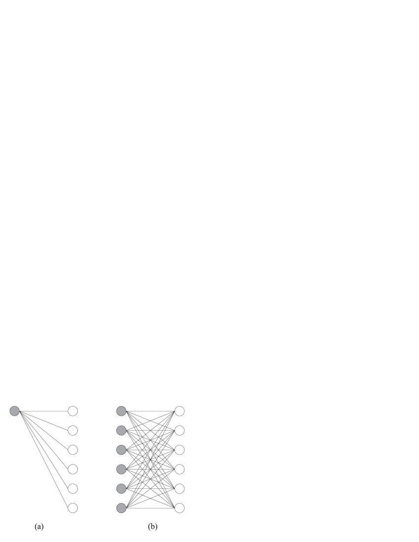
Figure 1: Figure 1: Schema of the interactions among the particles of the open system $A$ (grey circles) and of the open system $B$ (white circles): (a) original spin-bath model ($M=1$), and (b) generalized spin-bath model ($M\neq 1$).

In eq. (26), $H$ is written in its diagonal form; then, the energy eigenvectors are

$$\left|\Uparrow_{1}\right\rangle...\left|\Uparrow_{i}\right\rangle...\left|\Uparrow_{M-1}\right\rangle\left|\Uparrow_{M}\right\rangle\left|\uparrow_{1}\right\rangle...\left|\uparrow_{k}\right\rangle...\left|\uparrow_{N-1}\right\rangle\left|\uparrow_{N}\right\rangle$$

$$\left|\Uparrow_{1}\right\rangle...\left|\Uparrow_{i}\right\rangle...\left|\Uparrow_{M-1}\right\rangle\left|\Uparrow_{M}\right\rangle\left|\uparrow_{1}\right\rangle...\left|\uparrow_{k}\right\rangle...\left|\uparrow_{N-1}\right\rangle\left|\downarrow_{N}\right\rangle$$

$$...$$

$$\left|\Downarrow_{1}\right\rangle...\left|\Downarrow_{i}\right\rangle...\left|\Downarrow_{M-1}\right\rangle\left|\Downarrow_{M}\right\rangle\left|\downarrow_{1}\right\rangle...\left|\downarrow_{k}\right\rangle...\left|\downarrow_{N-1}\right\rangle\left|\downarrow_{N}\right\rangle$$ (27)

In turn, the eigenvectors of $H_{A}$ form a basis of $\mathcal{H}_{A}$. In order to simplify the expressions, we will introduce a particular arrangement into the set of those vectors, by calling them $\left|\mathcal{A}_{i}\right\rangle$: the set $\left\{\left|\mathcal{A}_{i}\right\rangle\right\}$ is an eigenbasis of $H_{A}$ with $2^{M}$ elements. The $\left|\mathcal{A}_{i}\right\rangle$ will be ordered in terms of the number $l\in\mathbb{N}_{0}$ of particles of $A$ having spin $\left|\Downarrow\right\rangle$. Then, we have that:

• $l=0$ corresponds to the unique state with all the particles with spin $\left|\Uparrow\right\rangle$:

  $$\left|\mathcal{A}_{1}\right\rangle=\left|\Uparrow,\Uparrow,...,\Uparrow,\Uparrow\right\rangle\Longrightarrow H_{A}\left|\mathcal{A}_{1}\right\rangle=\frac{M}{2}\left|\mathcal{A}_{1}\right\rangle$$ (28)

• $l=1$ corresponds to the $M$ states with only one particle with spin $\left|\Downarrow\right\rangle$. Since the order of the eigenvectors with the same eigenvalue will be irrelevant for the computations, we will order these states in an arbitrary way:

  $$\left|\mathcal{A}_{j}\right\rangle = \left|\Uparrow,\Uparrow,...,\Uparrow,\Downarrow,\Uparrow,...,\Uparrow,\Uparrow\right\rangle\Longrightarrow H_{A}\left|\mathcal{A}_{j}\right\rangle=\frac{M-2}{2}\left|\mathcal{A}_{j}\right\rangle$$

  $$\text{with \ \ }j = 2,3,...,M+1$$ (29)

• $l=2$ corresponds to the $\frac{\left(M-1\right)M}{2}$ states with two particles with spin $\left|\Downarrow\right\rangle$. Again, we will order these states in an arbitrary way:

  $$\left|\mathcal{A}_{j}\right\rangle =\left|\Uparrow,\Uparrow,,...,\Uparrow,\Downarrow,\Uparrow,,...,\Uparrow,\Downarrow,\Uparrow,...,\Uparrow,\Uparrow\right\rangle\Longrightarrow H_{A}\left|\mathcal{A}_{j}\right\rangle=\frac{M-4}{2}\left|\mathcal{A}_{j}\right\rangle$$

  $$\text{with \ \ }j =M+2,M+3,...,M+1+\frac{\left(M-1\right)M}{2}$$ (30)

• For the remaining values of $l$, the procedure is analogous.

Consequently, we have:

$$1\text{ eigenvector with eigenvalue }\frac{M}{2}$$

$$M\text{ eigenvectors with eigenvalue }\frac{M-2}{2}$$

$$\vdots$$

$$\frac{M!}{(M-l)!l!}\text{ eigenvectors with eigenvalue }\frac{M-2l}{2}$$ (31)

with $l=0,1,...M$. Then, it is clear that $H_{A}$ is degenerate: it has $2^{M}$ eigenvectors but only $M$ different eigenvalues. Therefore, a generic state $\left|\mathcal{A}\right\rangle$ of the system $A$ can be written in the basis $\left\{\left|\mathcal{A}_{i}\right\rangle\right\}$ as

$$\left|\mathcal{A}\right\rangle=\sum_{i=1}^{2^{M}}C_{i}\left|\mathcal{A}_{i}\right\rangle\in\mathcal{H}_{A}\text{ \ \qquad\ with \ \ }\sum_{i=1}^{2^{M}}\left|C_{i}\right|^{2}=1$$ (32)

By introducing eq. (32) into eq. (25), a pure initial state of the composite system $U=A\cup B$ reads

$$\left|\psi_{0}\right\rangle=\left(\sum_{i=1}^{2^{M}}C_{i}\left|\mathcal{A}_{i}\right\rangle\right)\otimes\left(\bigotimes_{k=1}^{N}\left(\alpha_{k}\left|\uparrow_{k}\right\rangle+\beta_{k}\left|\downarrow_{k}\right\rangle\right)\right)$$ (33)

If we group the degrees of freedom of $B$ in a single ket $\left|\mathcal{B}(0)\right\rangle$, $\left|\psi_{0}\right\rangle$ results

$$|\psi_{0}\rangle=\sum_{i=1}^{2^{M}}C_{i}\left|\mathcal{A}_{i}\right\rangle\otimes\left|\mathcal{B}(0)\right\rangle$$ (34)

The time-evolution of $|\psi(t)\rangle$ is ruled by the time-evolution operator $\mathcal{U}(t)=e^{-iHt}=e^{-i(H_{A}\otimes H_{B})t}$:

$$|\psi(t)\rangle=\mathcal{U}(t)|\psi_{0}\rangle=\sum_{i=1}^{2^{M}}C_{i}\,e^{-i(H_{A}\otimes H_{B})t}\,\left|\mathcal{A}_{i}\right\rangle\otimes\left|\mathcal{B}(0)\right\rangle=\sum_{i=1}^{2^{M}}C_{i}\,e^{-iH_{A}t}\,\left|\mathcal{A}_{i}\right\rangle\otimes e^{-iH_{B}t}\,\left|\mathcal{B}(0)\right\rangle$$ (35)

If we use $\Lambda_{k}$ to denote the eigenvalue of $H_{A}$ corresponding to the eigenvector $\left|\mathcal{A}_{k}\right\rangle$, then

$$|\psi(t)\rangle=\sum_{i=1}^{2^{M}}C_{i}\,\left|\mathcal{A}_{i}\right\rangle\otimes e^{-i\Lambda_{i}H_{B}t}\,\left|\mathcal{B}(0)\right\rangle=\sum_{i=1}^{2^{M}}C_{i}\,\left|\mathcal{A}_{i}\right\rangle\otimes\left|\mathcal{B}(t)\right\rangle$$ (36)

where (see eq. (26))

$$\left|\mathcal{B}(t)\right\rangle=e^{-i\Lambda_{i}H_{B}t}\,\left|\mathcal{B}(0)\right\rangle=\exp\left[-i\Lambda_{k}\sum\limits_{j=1}^{N}g_{j}\left(\left|\uparrow_{j}\right\rangle\left\langle\uparrow_{j}\right|-\left|\downarrow_{j}\right\rangle\left\langle\downarrow_{j}\right|\right)t\right]\left|\mathcal{B}(0)\right\rangle$$ (37)

Since the number of the eigenstates of $H_{A}$ with the same eigenvalue is given by eqs. (31), the terms of $|\psi(t)\rangle$ can be arranged as

$$\left|\psi(t)\right\rangle =\left(C_{1}\left|\mathcal{A}_{1}\right\rangle\left|\mathcal{B}_{0}(t)\right\rangle\right)+\left(\sum\limits_{\lambda=1}^{M+1}C_{\lambda}\left|\mathcal{A}_{\lambda}\right\rangle\left|\mathcal{B}_{1}(t)\right\rangle\right)+\left(\sum\limits_{\lambda=M+2}^{M+1+\frac{\left(M-1\right)M}{2}}C_{\lambda}\left|\mathcal{A}_{\lambda}\right\rangle\left|\mathcal{B}_{2}(t)\right\rangle\right)+...+$$

$$+\left(\sum\limits_{\lambda=1+\sum_{p=0}^{l-1}\binom{M}{P}}^{\sum_{p=0}^{l}\binom{M}{P}}C_{\lambda}\left|\mathcal{A}_{\lambda}\right\rangle\left|\mathcal{B}_{l}(t)\right\rangle\right)+...+\left(C_{2^{M}}\left|\mathcal{A}_{2^{M}}\right\rangle\left|\mathcal{B}_{M}(t)\right\rangle\right)$$ (38)

where

$$\left|\mathcal{B}_{l}(t)\right\rangle=\bigotimes\limits_{k=1}^{N}\left(\alpha_{k}e^{i\frac{\left(2l-M\right)}{2}g_{k}t}\left|\uparrow_{k}\right\rangle+\beta_{k}e^{-i\frac{\left(2l-M\right)}{2}g_{k}t}\left|\downarrow_{k}\right\rangle\right)$$ (39)

If we compare eq. (39) with eq. (4), we can see that $\left|\mathcal{E}_{\Uparrow}(t)\right\rangle$ and $\left|\mathcal{E}_{\Downarrow}(t)\right\rangle$ are the particular cases of $\left|\mathcal{B}_{l}(t)\right\rangle$ for $M=1$ and, then, $l=0,1$. Let us recall that $l$ is the number of particles of the system $A$ having spin $\left|\Downarrow\right\rangle$. Then, with $M=1$ and $l=0$, $\left|\mathcal{B}_{l}(t)\right\rangle=\left|\mathcal{E}_{\Uparrow}(t)\right\rangle$, and with $M=1$ and $l=1$, $\left|\mathcal{B}_{l}(t)\right\rangle=\left|\mathcal{E}_{\Downarrow}(t)\right\rangle$.

If we define the function

$$f(l)=\QATOPD\{\}{\sum_{p=0}^{l}\binom{M}{P}\text{ if }l=0,1,...,M}{0\text{ \ \ \ \ \ \ \ \ \ \ otherwise}}$$ (40)

then eq. (38) can be rewritten as

$$\left|\psi(t)\right\rangle=\sum\limits_{l=0}^{M}\sum\limits_{\lambda=f(l-1)+1}^{f(l)}C_{\lambda}\left|\mathcal{A}_{\lambda}\right\rangle\left|\mathcal{B}_{l}(t)\right\rangle$$ (41)

and the state operator $\rho(t)=\left|\psi(t)\right\rangle\left\langle\psi(t)\right|$ reads

$$\rho(t)=\sum\limits_{l,l^{\prime}=0}^{M}\sum\limits_{\QATOP{\lambda=f(l-1)+1}{\lambda^{\prime}=f(l^{\prime}-1)+1}}^{\QATOP{f(l)}{f(l^{\prime})}}C_{\lambda}C_{\lambda^{\prime}}^{\ast}\left|\mathcal{A}_{\lambda}\right\rangle\left|\mathcal{B}_{l}(t)\right\rangle\left\langle\mathcal{B}_{l^{\prime}}(t)\right|\left\langle\mathcal{A}_{\lambda^{\prime}}\right|$$ (42)

An observable $O\in\mathcal{O}=\mathcal{H}\otimes\mathcal{H}$ of the closed system $U=A\cup B$ can be expressed as

$$O=\left(\sum\limits_{\lambda,\lambda^{\prime}=0}^{2^{M}}s_{\lambda,\lambda^{\prime}}\left|\mathcal{A}_{\lambda}\right\rangle\left\langle\mathcal{A}_{\lambda^{\prime}}\right|\right)\otimes\left(\bigotimes_{i=1}^{N}\left(\epsilon_{\uparrow\uparrow}^{(i)}\left|\uparrow_{i}\right\rangle\left\langle\uparrow_{i}\right|+\epsilon_{\uparrow\downarrow}^{(i)}\left|\uparrow_{i}\right\rangle\left\langle\downarrow_{i}\right|+\epsilon_{\downarrow\uparrow}^{(i)}\left|\downarrow_{i}\right\rangle\left\langle\uparrow_{i}\right|+\epsilon_{\downarrow\downarrow}^{(i)}\left|\downarrow_{i}\right\rangle\left\langle\downarrow_{i}\right|\right)\right)$$ (43)

Let us notice that eq. (5) (a generic observable in the original spin-bath model) is a particular case of this eq. (43), with only four terms in the first factor. Analogously to that case, the diagonal components $s_{\lambda,\lambda}$, $\epsilon_{\uparrow\uparrow}^{(i)}$, $\epsilon_{\downarrow\downarrow}^{(i)}$ are real numbers, and the off-diagonal components are complex numbers satisfying $s_{\lambda,\lambda^{\prime}}=s_{\lambda^{\prime},\lambda}^{\ast}$, $\epsilon_{\uparrow\downarrow}^{(i)}=\epsilon_{\downarrow\uparrow}^{(i)\ast}$. Then, the expectation value of the observable $O$ in the state $\rho(t)$ of eq. (42) can be computed as

$$\langle O\rangle_{\rho(t)}=Tr\left(O\rho(t)\right)=\sum\limits_{l,l^{\prime}=0}^{M}\sum\limits_{\QATOP{\lambda=f(l-1)+1}{\lambda^{\prime}=f(l^{\prime}-1)+1}}^{\QATOP{f(l)}{f(l^{\prime})}}B_{\lambda,\lambda^{\prime}}T_{l,l^{\prime}}(t)$$ (44)

where

$$T_{l,l^{\prime}}(t)=\prod_{j=1}^{N}\left[\left|\alpha_{j}\right|^{2}\epsilon_{\uparrow\uparrow}^{(j)}e^{i\left(g_{j,l}-g_{j,l^{\prime}}\right)\frac{t}{2}}+\left|\beta_{j}\right|^{2}\epsilon_{\downarrow\downarrow}^{(j)}e^{-i\left(g_{j,l}-g_{j,l^{\prime}}\right)\frac{t}{2}}+2\mathop{\mathrm{R}e}\left(\alpha_{j}\beta_{j}^{\ast}\epsilon_{\downarrow\uparrow}^{(j)}e^{i\left(g_{j,l}+g_{j,l^{\prime}}\right)\frac{t}{2}}\right)\right]$$ (45)

and

$$g_{j,l}=\left(2l-M\right)g_{j}\text{, \ \qquad\ }B_{\lambda,\lambda^{\prime}}=C_{\lambda}C_{\lambda^{\prime}}^{\ast}s_{\lambda^{\prime},\lambda}$$ (46)

Since the exponents in eq. (45) are of the form $g_{j,l}\pm g_{j,l^{\prime}}$, in some cases they are zero. So, we can write

$$\langle O\rangle_{\rho(t)}=\sum\limits_{l=0}^{M}\sum\limits_{\QATOP{\lambda=f(l-1)+1}{\lambda^{\prime}=f(l-1)+1}}^{f(l)}B_{\lambda,\lambda^{\prime}}T_{l,l}(t)+\sum\limits_{l=0}^{\tilde{M}}\sum\limits_{\QATOP{\lambda=f(l-1)+1}{\lambda^{\prime}=f(M-l-1)+1}}^{\QATOP{f(l)}{f(M-l)}}B_{\lambda,\lambda^{\prime}}2\mathop{\mathrm{R}e}\left(T_{l,M-l}(t)\right)+\sum\limits_{\QATOP{\QATOP{l,l^{\prime}=0}{l\neq l^{\prime}}}{l^{\prime}\neq M-l}}^{M}\sum\limits_{\QATOP{\lambda=f(l-1)+1}{\lambda^{\prime}=f(l-1)+1}}^{\QATOP{f(l)}{f(l^{\prime})}}B_{\lambda,\lambda^{\prime}}T_{l,l^{\prime}}(t)$$ (47)

where

$$\tilde{M}=\QATOPD\{\}{\frac{M-2}{2}\text{ if }M\text{ is even}}{\frac{M-1}{2}\text{\ if }M\text{ is odd}}$$ (48)

$$T_{l,l}(t)=\prod_{j=1}^{N}\left[\left|\alpha_{j}\right|^{2}\epsilon_{\uparrow\uparrow}^{(j)}+\left|\beta_{j}\right|^{2}\epsilon_{\downarrow\downarrow}^{(j)}+2\mathop{\mathrm{R}e}\left(\alpha_{j}\beta_{j}^{\ast}\epsilon_{\downarrow\uparrow}^{(j)}e^{ig_{j,l}t}\right)\right]$$ (49)

$$T_{l,M-l}(t)=\prod_{j=1}^{N}\left[\left|\alpha_{j}\right|^{2}\epsilon_{\uparrow\uparrow}^{(j)}e^{ig_{j,l}t}+\left|\beta_{j}\right|^{2}\epsilon_{\downarrow\downarrow}^{(j)}e^{-ig_{j,l}t}+2\mathop{\mathrm{R}e}\left(\alpha_{j}\beta_{j}^{\ast}\epsilon_{\downarrow\uparrow}^{(j)}\right)\right]$$ (50)

Let us notice that eqs. (49) and (50) are analogous to eqs. (9) and (10) for $\Gamma_{0}(t)$ and $\Gamma_{1}(t)$, respectively, in the original model, with $g_{j,l}=\left(2l-M\right)g_{j}$ instead of $g_{j}$. In particular, when $M=1$ and, so, $l=0,1$, then $T_{l,l}(t)=\Gamma_{0}(t)$ and $T_{l,M-l}(t)=\Gamma_{1}(t)$.

As in the case of the original spin-bath model, here we will consider different meaningful ways of selecting the relevant observables.

IV Generalized spin-bath model: Decomposition 1

IV.1 Selecting the relevant observables

In this case $A$ is the open system $S$ and $B$ is the environment $E$. This is a generalization of Decomposition 1 in the original spin-bath model. The only difference with respect to that case is that here the system $S$ is composed of $M\geq 1$ particles instead of only one. Then, the decomposition for this case is

$$\mathcal{H}=\mathcal{H}_{S}\otimes\mathcal{H}_{E}=\left(\bigotimes\limits_{i=1}^{M}\mathcal{H}_{A_{i}}\right)\otimes\left(\bigotimes\limits_{k=1}^{N}\mathcal{H}_{B_{k}}\right)$$ (51)

Therefore, the relevant observables $O_{R}$ of the closed system $U$ are those corresponding to $A$, and they are obtained from eq. (43) by making $\epsilon_{\uparrow\uparrow}^{(i)}=\epsilon_{\downarrow\downarrow}^{(i)}=1,$ $\epsilon_{\uparrow\downarrow}^{(i)}=0$ (compare with eq. (12) in the original spin-bath model):

$$O_{R}=O_{S}\otimes\mathbb{I}_{E}=\left(\sum\limits_{\lambda,\lambda^{\prime}=0}^{2^{M}}s_{\lambda,\lambda^{\prime}}\left|\mathcal{A}_{\lambda}\right\rangle\left\langle\mathcal{A}_{\lambda^{\prime}}\right|\right)\otimes\left(\bigotimes_{i=1}^{N}\mathbb{I}_{i}\right)$$ (52)

With this condition, the expectation values of these observables are given by eq. (47), with

$$T_{l,l}(t) = \prod_{j=1}^{N}\left(\left|\alpha_{j}\right|^{2}+\left|\beta_{j}\right|^{2}\right)=1$$ (53)

$$T_{l,M-l}(t) = \prod_{j=1}^{N}\left(\left|\alpha_{j}\right|^{2}e^{ig_{j,l}t}+\left|\beta_{j}\right|^{2}e^{-ig_{j,l}t}\right)$$ (54)

$$T_{l,l^{\prime}}(t) = \prod_{j=1}^{N}\left(\left|\alpha_{j}\right|^{2}e^{i\left(g_{j,l}-g_{j,l^{\prime}}\right)\frac{t}{2}}+\left|\beta_{j}\right|^{2}e^{-i\left(g_{j,l}-g_{j,l^{\prime}}\right)\frac{t}{2}}\right)$$ (55)

If we define the functions $R_{l}(t)=|T_{l,M-l}(t)|^{2}$ and $R_{ll^{\prime}}(t)=|T_{l,l^{\prime}}(t)|^{2}$, they result

$$R_{l}(t) = \prod_{j=1}^{N}\left(\left|\alpha_{j}\right|^{4}+\left|\beta_{j}\right|^{4}+2\left|\alpha_{j}\right|^{2}\left|\beta_{j}\right|^{2}\cos\left(2\left(2l-M\right)g_{j}t\right)\right)$$ (56)

$$R_{ll^{\prime}}(t) = \prod_{j=1}^{N}\left(\left|\alpha_{j}\right|^{4}+\left|\beta_{j}\right|^{4}+2\left|\alpha_{j}\right|^{2}\left|\beta_{j}\right|^{2}\cos\left(2\left(l-l^{\prime}\right)g_{j}t\right)\right)$$ (57)

We can see that $|r(t)|^{2}$ of eq. (15) in the original model is the particular case of $R_{l}(t)$ for $M=1$.

IV.2 Computing the behavior of the relevant expectation values

The expectation value given by eq. (47) has three terms, $\langle O_{R}\rangle_{\rho(t)}=\Sigma^{\left(1\right)}+\Sigma^{\left(2\right)}+\Sigma^{\left(3\right)}$, which can be analyzed separately:

• From eq. (53), the first term reads

  $$\Sigma^{\left(1\right)}=\sum\limits_{l=0}^{M}\sum\limits_{\lambda,\lambda^{\prime}=f(l-1)+1}^{f(l)}B_{\lambda,\lambda^{\prime}}=\sum\limits_{l=0}^{M}\sum\limits_{\lambda,\lambda^{\prime}=f(l-1)+1}^{f(l)}C_{\lambda}C_{\lambda^{\prime}}^{\ast}s_{\lambda^{\prime},\lambda}\neq\Sigma^{\left(1\right)}(t)$$ (58)

  It is clear that this first term does not evolve with time.

• The time-dependence of the second term is given by $T_{l,M-l}(t)$:

  $$\Sigma^{\left(2\right)}(t)=\sum\limits_{l=0}^{\tilde{M}}\sum\limits_{\QATOP{\lambda=f(l-1)+1}{\lambda^{\prime}=f(M-l-1)+1}}^{\QATOP{f(l)}{f(M-l)}}B_{\lambda,\lambda^{\prime}}2\mathop{\mathrm{R}e}\left(T_{l,M-l}(t)\right)$$ (59)

  Then, in order to obtain the limit of this term, we have to compute the limit of $R_{l}(t)=|T_{l,M-l}(t)|^{2}$ of eq. (56). As in the case of the original spin-bath model, here we take $\left|\alpha_{j}\right|^{2}$ and $\left|\beta_{ji}\right|^{2}$ as random numbers in the closed interval $\left[0,1\right]$, such that $|\alpha_{j}|^{2}+|\beta_{j}|^{2}=1$. Then

  $$\max_{t}\left(\left|\alpha_{j}\right|^{4}+\left|\beta_{j}\right|^{4}+2\left|\alpha_{j}\right|^{2}\left|\beta_{j}\right|^{2}\cos\left(2\left(2l-M\right)g_{j}t\right)\right) = 1$$ (60)

  $$\min_{t}\left(\left|\alpha_{j}\right|^{4}+\left|\beta_{j}\right|^{4}+2\left|\alpha_{j}\right|^{2}\left|\beta_{j}\right|^{2}\cos\left(2\left(2l-M\right)g_{j}t\right)\right) = \left(2\left|\alpha_{j}\right|^{2}-1\right)^{2}$$ (61)

  Therefore, $\left[\left|\alpha_{j}\right|^{4}+\left|\beta_{j}\right|^{4}+2\left|\alpha_{j}\right|^{2}\left|\beta_{j}\right|^{2}\cos\left(2\left(2l-M\right)g_{j}t\right)\right]$ is a random number which, if $t\neq 0$, fluctuates between $1$ and $\left(2\left|\alpha_{j}\right|^{2}-1\right)^{2}$. Again, when the environment has many particles (that is, when $N\rightarrow\infty$), the statistical value of the cases $\left|\alpha_{j}\right|^{2}=1$, $\left|\beta_{j}\right|^{2}=1$, $\left|\alpha_{j}\right|^{2}=0$ and $\left|\beta_{j}\right|^{2}=0$ tends to zero. In this situation, eq. (56) for $R_{l}(t)$ is an infinite product of numbers belonging to the open interval $\left(0,1\right)$.  As a consequence, when $N\rightarrow\infty$, $R_{l}(t)\rightarrow 0$.

• The time-dependence of the third term is given by $T_{l,l^{\prime}}(t)$:

  $$\Sigma^{\left(3\right)}(t)=\sum\limits_{\QATOP{\QATOP{l,l^{\prime}=0}{l\neq l^{\prime}}}{l^{\prime}\neq M-l}}^{M}\sum\limits_{\QATOP{\lambda=f(l-1)+1}{\lambda^{\prime}=f(l^{\prime}-1)+1}}^{\QATOP{f(l)}{f(l^{\prime})}}B_{\lambda,\lambda^{\prime}}T_{l,l^{\prime}}(t)$$ (62)

  with the restrictions on $l$ and $l^{\prime}$: $\ l\neq l^{\prime}$ and $l^{\prime}\neq M-l$. As in the second term, we have to compute the limit of $R_{ll^{\prime}}(t)=|T_{l,l^{\prime}}(t)|^{2}$ of eq. (57) and, on the basis of an analogous argument, the result is the same as above: when $N\rightarrow\infty$, $R_{ll^{\prime}}(t)\rightarrow 0$.

If we want now to evaluate the limit of $\langle O_{R}\rangle_{\rho(t)}$ for $t\rightarrow\infty$, we have to compute the limits of the second and the third terms (since the first term, as we have seen, is time-independent). Here we have to distinguish three cases: $M\ll N$, $M\gg N$ and $M\simeq N$.

Case (a): $M\ll N$

This case is similar to Decomposition 1 in the original spin-bath model, since in both cases $M\ll N$: the only difference is that in the original model $M=1$ whereas here $M\geq 1$.

In fact, we have seen that $T_{l,M-l}(t)$ is analogous to $\Gamma_{1}(t)$ in the original model. Moreover, $T_{l,l^{\prime}}(t)$ has the same functional form as $\Gamma_{1}(t)$. In paper Max it is shown that $\Gamma_{1}(t)$ approaches zero for $t\rightarrow\infty$. This means that we can infer that $T_{l,M-l}(t)$ and $T_{l,l^{\prime}}(t)$ also approach zero for $t\rightarrow\infty$. On the other hand, the terms $\Sigma^{\left(2\right)}(t)$ and $\Sigma^{\left(3\right)}(t)$ are sums of less than $M$ terms involving $T_{l,M-l}(t)$ and $T_{l,l^{\prime}}(t)$. As a consequence, since in this case $M$ is a small number, the sum of a small number of terms approaching zero for $t\rightarrow\infty$ also approaches zero: $\lim_{t\rightarrow\infty}\Sigma^{\left(2\right)}(t)=0$ and $\lim_{t\rightarrow\infty}\Sigma^{\left(3\right)}(t)=0$. Therefore,

$$\lim_{t\rightarrow\infty}\langle O_{R}\rangle_{\rho(t)}=\lim_{t\rightarrow\infty}\left[\Sigma^{\left(1\right)}(t)+\Sigma^{\left(2\right)}(t)+\Sigma^{\left(3\right)}(t)\right]=\Sigma^{\left(1\right)}(t)$$ (63)

In other words,

$$\lim_{t\rightarrow\infty}\langle O_{R}\rangle_{\rho(t)}=\sum\limits_{l=0}^{M}\sum\limits_{\lambda,\lambda^{\prime}=f(l-1)+1}^{f(l)}B_{\lambda,\lambda^{\prime}}=\sum\limits_{l=0}^{M}\sum\limits_{\lambda,\lambda^{\prime}=f(l-1)+1}^{f(l)}C_{\lambda}C_{\lambda^{\prime}}^{\ast}s_{\lambda^{\prime},\lambda}=\langle O_{R}\rangle_{\rho_{\ast}}$$ (64)

where $\rho_{\ast}$ is the final diagonal state of $U$. This result can also be expressed in terms of the reduced density operator $\rho_{A}$ of the system $A$ as:

$$\lim_{t\rightarrow\infty}\langle O_{R}\rangle_{\rho(t)}=\langle O_{R}\rangle_{\rho_{\ast}}=\lim_{t\rightarrow\infty}\langle O_{A}\rangle_{\rho_{A}(t)}=\langle O_{A}\rangle_{\rho_{A\ast}}$$ (65)

In the eigenbasis of the Hamiltonian $H_{A}$ of $A$, the final reduced density operator $\rho_{A\ast}$ is expressed by a $2^{M}\times 2^{M}$ matrix:

$$\rho_{A\ast}=\begin{pmatrix}\rho_{l=0}&0&0&0&...&0\\ 0&\rho_{l=1}&0&0&...&0\\ 0&0&\rho_{l=2}&0&...&0\\ 0&0&0&\rho_{l=3}&...&0\\ ...&...&...&...&...&...\\ 0&0&0&0&0&\rho_{l=M}\end{pmatrix}$$ (66)

where $\rho_{l=0}=\left|C_{1}\right|^{2}$ and each $\rho_{l}$ is a matrix of dimension $\frac{M!}{\left(M-l\right)!l!}\times\frac{M!}{\left(M-l\right)!l!}$. This result might seem insufficient for decoherence because, since the $\rho_{l}$ are matrices, $\rho_{A\ast}$ seems to be non completely diagonal in the eigenbasis of the Hamiltonian $H_{A}$. However, we have to recall that all the states $\left|\mathcal{A}_{i}\right\rangle$ with same $l$ are degenerate eigenvectors corresponding to the same eigenvalue of $H_{A}$; then, the basis that diagonalizes $\rho_{A\ast}$ (i.e., that diagonalizes all the matrices $\rho_{l}$) is an eigenbasis of $H_{A}$. Summing up, the system $S=A$ of $M$ particles in interaction with its environment $E=B$ of $N\gg M$ particles decoheres in the eigenbasis of $\rho_{A\ast}$, which is also an eigenbasis of $H_{A}$.

If we want to compute the time-behavior of $\langle O_{R}\rangle_{\rho(t)}$, we have to consider that $\Sigma^{\left(1\right)}$ is a sum of terms of the form $(B_{\lambda,\lambda^{\prime}}\left|\alpha_{j}\right|^{2}+B_{\lambda,\lambda^{\prime}}\left|\beta_{j}\right|^{2})$, that is, terms of the expectation value coming from the diagonal part of $\rho(t)$ in the basis of the Hamiltonian $H$. Therefore, if there is decoherence, the sum $\Sigma^{nd}(t)=\Sigma^{\left(2\right)}+\Sigma^{\left(3\right)}$, involving the terms of $\langle O_{R}\rangle_{\rho(t)}$ coming from the non-diagonal part of $\rho(t)$, has to approach zero for $t\rightarrow\infty$.

In order to show an example of the time-behavior of $\langle O_{R}\rangle_{\rho(t)}$, numerical simulations for $\Sigma^{nd}(t)$ have been performed, with the following features:

1. $s_{\lambda^{\prime},\lambda}=1$ (see eq. (52)).

2. The initial condition for $S=A$ is selected as (see eq. (32)) :

   $$\left|\mathcal{A}\right\rangle=\frac{1}{\sqrt{2^{M}}}\sum_{i=1}^{2^{M}}\left|\mathcal{A}_{i}\right\rangle\Longrightarrow\forall\lambda,\ C_{\lambda}=C_{\lambda}^{\ast}=\frac{1}{\sqrt{2^{M}}}\Longrightarrow C_{\lambda}C_{\lambda^{\prime}}^{\ast}=\frac{1}{2^{M}}$$ (67)

   Then, from (i) and (ii), $B_{\lambda,\lambda^{\prime}}=2^{-M}$ (see eq. (46)).

3. $\left|\alpha_{i}\right|^{2}$ is generated by a random-number generator in the interval $[0,1]$, and $\left|\beta_{i}\right|^{2}$ is obtained as $\left|\beta_{i}\right|^{2}=1-\left|\alpha_{i}\right|^{2}$.

4. $g_{i}=400Hz$: as explained above, the coupling constant in typical models of spin interaction.

5. As in the original model, the time-interval $\left[0,t_{0}\right]$ was partitioned into intervals $\Delta t=t_{0}/200$, and the function $\Sigma^{nd}(t)$ was computed at times $t_{k}=k\Delta t$, with $k=0,1,...,200$.

6. $N=10^{3}$, and $M=1$ and $M=10$.

Figure 2 shows the time-evolution of $\Sigma^{nd}(t)$.

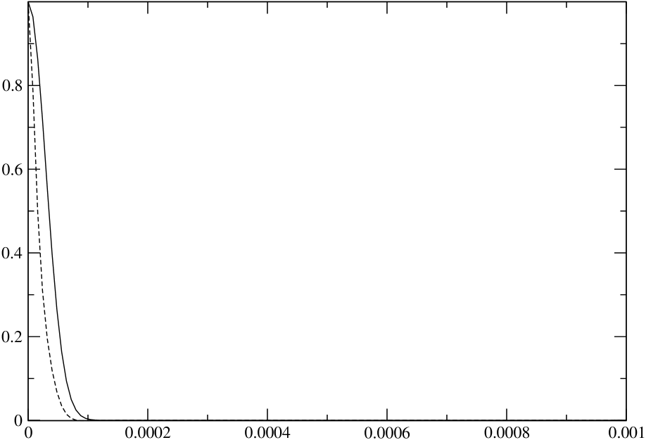
Figure 2: Figure 2: Evolution of $\Sigma^{nd}(t)$ for $N=10^{3}$, and $M=1$ (solid line) and $M=10$ (dash line), with $t_{0}=10^{-3}s$.

This result shows that, as expected, a small open system $S=A$ of $M$ particles decoheres in interaction with a large environment $E=B$ of $N\gg M$ particles.

Case (b): $M\gg N$

In this case, where the open system $S=$ $A$ has much more particles than the environment $E=B$, the argument of Case (a) cannot be applied: since now $\Sigma^{\left(2\right)}(t)$ and $\Sigma^{\left(3\right)}(t)$ are no longer sums over a small number of terms, the fact that each term approaches zero does not guarantee that the sums also approach zero. In particular, if $N=1$, then (see eq. (55))

$$T_{l,l^{\prime}}(t)=\left|\alpha_{1}\right|^{2}e^{i\left(g_{1,l}-g_{1,l^{\prime}}\right)\frac{t}{2}}+\left|\beta_{1}\right|^{2}e^{-i\left(g_{1,l}-g_{1,l^{\prime}}\right)\frac{t}{2}}$$ (68)

which clearly has no limit for $t\rightarrow\infty$. Nevertheless, it might happen that, with $N$ high but $M$ much higher than $N$, each term of the sums approaches zero. So, in order to know the time behavior of $\langle O_{R}\rangle_{\rho(t)}$, numerical simulations for $\Sigma^{nd}(t)$ have been performed, with the same features as in the previous case, with the exception of condition (vi), which was taken as:

1. $M=10^{3}$, and $N=10$ and $N=100$.

Figure 3 shows the time-evolution of $\Sigma^{nd}(t)$ in this case.

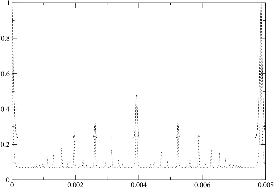
Figure 3: Figure 3: Evolution of $\Sigma^{nd}(t)$ for $M=10^{3}$, and $N=10$ (dash line) and $N=100$ (dot line), with $t_{0}=10^{-3}s$.

This result is also what may be expected: when  the open system $S=A$ of $M$ particles is larger that the environment $E=B$ of $N\ll M$ particles, $S$ does not decohere.

Case (c): $M\simeq N$

In this case, where the numbers of particles of the open system $S=$ $A$ and of the environment $E=B$ do not differ in more than one order of magnitude, the time behavior of $\langle O_{R}\rangle_{\rho(t)}$ cannot be inferred from the equations. Numerical simulations have been performed, with the same features as in Case (b), with the exception of condition (vi), which was taken as:

1. $N=10^{3}$, and $M=10^{2}$ and $M=10^{3}$.

Figure 4 shows the time-evolution of $\Sigma^{nd}(t)$.

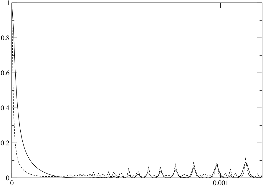
Figure 4: Figure 4: Evolution of $\Sigma^{nd}(t)$ for $N=10^{3}$, and $M=10^{2}$ (dash line) and $M=10^{3}$ (solid line), with $t_{0}=12.10^{-4}s$.

Again, if the environment $E=B$ of $N$ particles is not large enough when compared with the open system $S=A$ of $M$ particles, $S$ does not decohere. Let us notice that, for $N=10^{3}$, the system $S=A$ with $M=10^{2}$ does not decohere (Figure 4), whereas it does decohere with $M=10$ (Figure 2). This shows that, in the case of this decomposition, $M\ll N$ means that $N$ is at least two orders of magnitude higher than $M$.

Summarizing results

Up to now, in this Decomposition 1 all the arguments were directed to know whether the system $A$ of $M$ particles decoheres or not in interaction with the system $B$ of $N$ particles. But, given the symmetry of the whole system, the same arguments can be used to decide whether the system $B$ of $N$ particles decoheres or not in interaction with the system $A$ of $M$ particles, with analogous results: $B$ decoheres only when $M\gg N$; if $M\ll N$ or $M\simeq N$, $B$ does not decohere. Therefore, all the results obtained in this section can be summarized as follows:

1. If $M\ll N$, $A$ decoheres and $B$ does not decohere.

2. If $M\gg N$, $A$ does not decohere and $B$ decoheres.

3. If $M\simeq N$, neither $A$ nor $B$ decohere.

V Generalized spin-bath model: Decomposition 2

V.1 Selecting the relevant observables

In this case we decide to observe only one particle of the open system $A$. This amounts to splitting the closed system $U$ into two new subsystems: the open system $S$ is, say, the particle $A_{M}$ with ket $\left|\Uparrow,\Uparrow,...,\Uparrow,\Uparrow,\Uparrow,\Downarrow\right\rangle$, and the environment is $E=\left(\cup_{i=1}^{M-1}A_{i}\right)\cup B=\left(\cup_{i=1}^{M-1}A_{i}\right)\cup\left(\cup_{k=1}^{N}B_{k}\right)$. The decomposition for this case is

$$\mathcal{H}=\mathcal{H}_{S}\otimes\mathcal{H}_{E}=\left(\mathcal{H}_{A_{M}}\right)\otimes\left(\left(\bigotimes\limits_{i=1}^{M-1}\mathcal{H}_{A_{i}}\right)\otimes\left(\bigotimes\limits_{k=1}^{N}\mathcal{H}_{B_{k}}\right)\right)$$ (69)

Therefore, the relevant observables $O_{R}$ of the closed system $U$ are those corresponding to the particle $A_{M}$:

$$O_{R}=O_{S}\otimes\mathbb{I}_{E}=\left(\sum\limits_{\alpha,\alpha^{\prime}=\Uparrow,\Downarrow}s_{\alpha,\alpha^{\prime}}\left|\alpha\right\rangle\left\langle\alpha^{\prime}\right|\right)\otimes\left(\left(\bigotimes_{i=1}^{M-1}\mathbb{I}_{i}\right)\otimes\left(\bigotimes_{k=1}^{N}\mathbb{I}_{k}\right)\right)$$ (70)

It is easy to see that the relevant observables selected in this Decomposition 2 form a subspace of the space of the relevant observables selected in Decomposition 1: eq. (70) can be obtained from eq. (52) by making $s_{\lambda,\lambda^{\prime}}=1$ for $\lambda=\lambda^{\prime}$ and $s_{\lambda,\lambda^{\prime}}=0$ for $\lambda\neq\lambda^{\prime}$ in all the terms of the sum except for the terms corresponding to the particle $A_{M}$.

In order to simplify expressions, in this case it is convenient to introduce a new arrangement for the eigenvectors of the Hamiltonian $H_{A}$, by calling them $\left|\mathcal{\tilde{A}}_{i}\right\rangle$: the set $\left\{\left|\mathcal{\tilde{A}}_{i}\right\rangle\right\}$ is an eigenbasis of $H_{A}$ with $2^{M}$ elements. The $\left|\mathcal{\tilde{A}}_{i}\right\rangle$ will be ordered by analogy with the binary numbers:

$$\left|\mathcal{\tilde{A}}_{1}\right\rangle = \left|\Uparrow,\Uparrow,...,\Uparrow,\Uparrow,\Uparrow,\Uparrow\right\rangle\text{, }\left|\mathcal{\tilde{A}}_{2}\right\rangle=\left|\Uparrow,\Uparrow,...,\Uparrow,\Uparrow,\Uparrow,\Downarrow\right\rangle\text{, }\left|\mathcal{\tilde{A}}_{3}\right\rangle=\left|\Uparrow,\Uparrow,...,\Uparrow,\Uparrow,\Downarrow,\Uparrow\right\rangle\text{,}$$

$$\text{ }\left|\mathcal{\tilde{A}}_{4}\right\rangle = \left|\Uparrow,\Uparrow,...,\Uparrow,\Uparrow,\Downarrow,\Downarrow\right\rangle\text{, }\left|\mathcal{\tilde{A}}_{5}\right\rangle=\left|\Uparrow,\Uparrow,...,\Uparrow,\Downarrow,\Uparrow,\Uparrow\right\rangle\text{, }\left|\mathcal{\tilde{A}}_{6}\right\rangle=\left|\Uparrow,\Uparrow,...,\Uparrow,\Downarrow,\Uparrow,\Downarrow\right\rangle,...$$

$$\left|\mathcal{\tilde{A}}_{2^{M}}\right\rangle = \left|\Downarrow,\Downarrow,...,\Downarrow,\Downarrow,\Downarrow,\Downarrow\right\rangle$$ (71)

According to this arrangement, the $\left|\mathcal{\tilde{A}}_{i}\right\rangle$ with even $i$ have the spin $M$ in the state $\left|\Downarrow\right\rangle$, and the $\left|\mathcal{\tilde{A}}_{i}\right\rangle$ with odd $i$ have the spin $M$ in the state $\left|\Uparrow\right\rangle$. So, the relevant observables of eq. (70) can be rewritten in terms of the $\left|\mathcal{\tilde{A}}_{i}\right\rangle$ as

$$O_{R}=\left(\sum\limits_{\lambda=1}^{2^{M}}\left(\tilde{s}_{\Uparrow\Uparrow}\left|\mathcal{\tilde{A}}_{2\lambda}\right\rangle\left\langle\mathcal{\tilde{A}}_{2\lambda}\right|+\tilde{s}_{\Uparrow\Downarrow}\left|\mathcal{\tilde{A}}_{2\lambda}\right\rangle\left\langle\mathcal{\tilde{A}}_{2\lambda-1}\right|+\tilde{s}_{\Downarrow\Uparrow}\left|\mathcal{\tilde{A}}_{2\lambda-1}\right\rangle\left\langle\mathcal{\tilde{A}}_{2\lambda}\right|+\tilde{s}_{\Downarrow\Downarrow}\left|\mathcal{\tilde{A}}_{2\lambda-1}\right\rangle\left\langle\mathcal{\tilde{A}}_{2\lambda-1}\right|\right)\right)\otimes\left(\bigotimes_{k=1}^{N}\mathbb{I}_{k}\right)$$ (72)

V.2 Computing the behavior of the relevant expectation values

Here the expectation values of the relevant observables are given by eq. (47), with $T_{l,l^{\prime}}(t)$, $T_{l,l}(t)$ and $T_{l,M-l}(t)$ given by eqs. (45), (49) and (50) respectively, but now replacing $B_{\lambda,\lambda^{\prime}}$ with $\tilde{B}_{\lambda,\lambda^{\prime}}$,

$$\langle O_{R}\rangle_{\rho(t)}=\sum\limits_{l=0}^{M}\sum\limits_{\QATOP{\lambda=f(l-1)+1}{\lambda^{\prime}=f(l-1)+1}}^{f(l)}\tilde{B}_{\lambda,\lambda^{\prime}}+\sum\limits_{l=0}^{\tilde{M}}\sum\limits_{\QATOP{\lambda=f(l-1)+1}{\lambda^{\prime}=f(M-l-1)+1}}^{\QATOP{f(l)}{f(M-l)}}\tilde{B}_{\lambda,\lambda^{\prime}}2\mathop{\mathrm{R}e}\left(T_{l,M-l}(t)\right)+\sum\limits_{\QATOP{\QATOP{l,l^{\prime}=0}{l\neq l^{\prime}}}{l^{\prime}\neq M-l}}^{M}\sum\limits_{\QATOP{\lambda=f(l-1)+1}{\lambda^{\prime}=f(l^{\prime}-1)+1}}^{\QATOP{f(l)}{f(l^{\prime})}}\tilde{B}_{\lambda,\lambda^{\prime}}T_{l,l^{\prime}}(t)$$ (73)

where the $\tilde{B}_{\lambda,\lambda^{\prime}}$ can be written in the basis $\left\{\left|\mathcal{\tilde{A}}_{\lambda}\right\rangle\right\}$ as

$$\tilde{B}_{\lambda,\lambda^{\prime}}=\left\{\begin{array}[]{ccccc}C_{\lambda}C_{\lambda^{\prime}}^{\ast}\tilde{s}_{\Uparrow\Uparrow}&\text{if}&\lambda&\text{is an even number and}&\lambda^{\prime}=\lambda\\ C_{\lambda}C_{\lambda^{\prime}}^{\ast}\tilde{s}_{\Uparrow\Downarrow}&\text{if}&\lambda&\text{is an even number and}&\lambda^{\prime}=\lambda-1\\ C_{\lambda}C_{\lambda^{\prime}}^{\ast}\tilde{s}_{\Downarrow\Uparrow}&\text{if}&\lambda&\text{is an odd number and}&\lambda^{\prime}=\lambda+1\\ C_{\lambda}C_{\lambda^{\prime}}^{\ast}\tilde{s}_{\Downarrow\Downarrow}&\text{if}&\lambda&\text{is an odd number and}&\lambda^{\prime}=\lambda\\ 0&&&\text{otherwise}&\end{array}\right\}$$ (74)

According to eq. (74), $\tilde{B}_{\lambda,\lambda^{\prime}}\neq 0$ only when

$$\lambda^{\prime}=\lambda\text{ \ \ \ \ or \ \ \ }\lambda^{\prime}=\lambda\pm 1\text{ }$$ (75)

Since $\lambda=f(l-1)+1$ and $\lambda^{\prime}=f(l^{\prime}-1)+1$, relations (75) imply that

$$l^{\prime}=l\text{ \ \ \ \ or \ \ \ }l^{\prime}=l\pm 1$$ (76)

The expectation value given by eq. (73) has again three terms, $\langle O\rangle_{\rho(t)}=\Sigma^{\left(1\right)}+\Sigma^{\left(2\right)}+\Sigma^{\left(3\right)}$, which can be analyzed separately:

• From eqs. (74) and (75), the first term reads

  $$\Sigma^{\left(1\right)}=\sum\limits_{l=0}^{M}\sum\limits_{\lambda=f(l-1)+1}^{f(l)}B_{\lambda,\lambda}=\sum\limits_{\lambda=0}^{2^{M-1}}\left(\left|C_{2\lambda}\right|^{2}\tilde{s}_{\Uparrow\Uparrow}+\left|C_{2\lambda+1}\right|^{2}\tilde{s}_{\Downarrow\Downarrow}\right)\neq\Sigma^{\left(1\right)}(t)$$ (77)

  Analogously to eq. (58) of Decomposition 1, this first term does not evolve with time.

• The time-dependence of the second term is given by $T_{l,M-l}(t)$. But with the restrictions of eqs. (75) and (76), $\Sigma^{\left(2\right)}$ has only two terms:

  $$\Sigma^{\left(2\right)}(t) = \sum\limits_{l=0}^{\tilde{M}}\sum\limits_{\QATOP{\lambda=f(l-1)+1}{\lambda^{\prime}=f(M-l-1)+1}}^{\QATOP{f(l)}{f(M-l)}}B_{\lambda,\lambda^{\prime}}2\mathop{\mathrm{R}e}\left(T_{l,M-l}(t)\right)=$$ (78)

  $$= C_{f(\frac{M-1}{2}-1)+1}C_{f(\frac{M-1}{2}-1)+2}^{\ast}\left(\tilde{s}_{\Downarrow\Uparrow}+\tilde{s}_{\Uparrow\Downarrow}\right)2\mathop{\mathrm{R}e}\left(T_{\frac{M-1}{2},\frac{M+1}{2}}(t)\right)$$ (79)

  Then, in order to obtain the limit of this term, we have to compute the limit of $T_{\frac{M-1}{2},\frac{M+1}{2}}(t)$, which is precisely the $T_{l,l^{\prime}}(t)$ of Decomposition 1 in the particular case that $l=\frac{M-1}{2}$ and $l^{\prime}=\frac{M+1}{2}$ (see eq. (55)). But, as we have seen in Case (a) of Decomposition 1, $T_{l,l^{\prime}}(t)$ has the same functional form as $\Gamma_{1}(t)$ of the original model (see eq. (10)), which approaches zero for $t\rightarrow\infty$ when $N\gg 1$. Therefore, for $N\gg 1$, $T_{\frac{M-1}{2},\frac{M+1}{2}}(t)$ also approaches zero for $t\rightarrow\infty$, and the same holds for $\Sigma^{\left(2\right)}(t)$ since it is a sum of two terms containing $T_{\frac{M-1}{2},\frac{M+1}{2}}(t)$.

• The time-dependence of the third term is given by $T_{l,l^{\prime}}(t)$. But with the restrictions of eqs. (75) and (76), $\Sigma^{\left(3\right)}$ results:

  $$\Sigma^{\left(3\right)}(t)=\sum\limits_{\QATOP{l=0}{l\neq\frac{M-1}{2}}}^{M}\sum\limits_{\lambda=f(l-1)+1}^{f(l)}\left(B_{\lambda,\lambda+1}T_{l,l+1}(t)+B_{\lambda,\lambda-1}T_{l,l-1}(t)\right)$$ (80)

  Since here $l^{\prime}=l\pm 1$ (see eq. (76)), in this case $T_{l,l\pm 1}(t)$ is:

  $$T_{l,l\pm 1}(t)=\prod_{j=1}^{N}\left(\left|\alpha_{j}\right|^{2}e^{\mp ig_{j}t}+\left|\beta_{j}\right|^{2}e^{\pm ig_{j}t}\right)$$ (81)

  If we compare this equation with eq. (14) for $r(t)$ in the original spin-bath model, we can see that

  $$T_{l,l+1}(t)=r(t)\text{ \ \ \ \ and \ \ \ }T_{l,l-1}(t)=r^{\ast}(t)$$ (82)

  Then,

  $$\Sigma^{\left(3\right)}(t)=\left(S_{+}r(t)+S_{-}r^{\ast}(t)\right)$$ (83)

  where $S_{+}$ and $S_{-}$ are constants given by

  $$S_{\pm}=\sum\limits_{\QATOP{l=0}{l\neq\frac{M-1}{2}}}^{M}\sum\limits_{\lambda=f(l-1)+1}^{f(l)}B_{\lambda,\lambda\pm 1}$$ (84)

  On the basis of the simulations of the original model we have seen that, when $N\gg 1$, $r(t)$ approaches zero for $t\rightarrow\infty$. Therefore, in this case we can conclude that, when $N\gg 1$, $\Sigma^{\left(3\right)}(t)$ approaches zero for $t\rightarrow\infty$.

Summing up, $\langle O_{R}\rangle_{\rho(t)}$ is the sum of three terms: one is time-independent and the other two tend to zero for $t\rightarrow\infty$. In particular, from eq. (77) we know that, for $N\gg 1$,

$$\lim_{t\rightarrow\infty}\langle O_{R}\rangle_{\rho(t)}=\sum\limits_{l=0}^{M}\sum\limits_{\lambda,\lambda^{\prime}=f(l-1)+1}^{f(l)}\tilde{B}_{\lambda,\lambda^{\prime}}=\sum\limits_{l=0}^{M}\sum\limits_{\lambda=0}^{2^{M-1}}\left(\left|C_{2\lambda}\right|^{2}\tilde{s}_{\Uparrow\Uparrow}+\left|C_{2\lambda+1}\right|^{2}\tilde{s}_{\Downarrow\Downarrow}\right)=\langle O_{R}\rangle_{\rho_{\ast}}$$ (85)

where $\rho_{\ast}$ is the final diagonal state of $U$. Again, this result can also be expressed in terms of the reduced density operator $\rho_{S}=\rho_{A_{M}}$ of the open system $S=A_{M}$ as (see eq. (65))

$$\lim_{t\rightarrow\infty}\langle O_{R}\rangle_{\rho(t)}=\langle O_{R}\rangle_{\rho_{\ast}}=\lim_{t\rightarrow\infty}\langle O_{A_{M}}\rangle_{\rho_{A_{M}}(t)}=\langle O_{A_{M}}\rangle_{\rho_{A_{M}\ast}}$$ (86)

where the final reduced density operator $\rho_{A_{M}\ast}$ in the basis $\{\left|\Uparrow\right\rangle,\left|\Downarrow\right\rangle\}$ reads

$$\rho_{A_{M}\ast}=\begin{pmatrix}\left|\alpha_{M}\right|^{2}&0\\ 0&\left|\beta_{M}\right|^{2}\end{pmatrix}$$ (87)

This shows that the open system $S=A_{M}$, composed of a single particle, decoheres in interaction with its environment $E$ of $N+M-1$ particles when $N\gg 1$, independently of the value of $M$.

In order to illustrate this conclusion, we have computed $\Sigma^{nd}(t)=\Sigma^{\left(2\right)}(t)+\Sigma^{\left(3\right)}(t)$ by means of numerical simulations with the same features as in Decomposition 1, with the exception of condition (vi), which was taken as:

Figure 5:   (vi) $\ M=10^{3}$ and $N=1$.

Figure 6:   (vi) $\ M=10^{3}$ and $N=10^{2}$.

Figure 7:   (vi) $\ M=10^{3}$ and $N=10^{3}$.

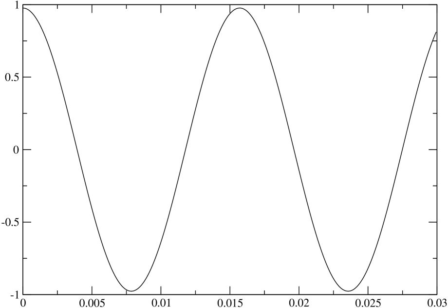
Figure 5: Figure 5: Evolution of $\Sigma^{nd}(t)$ for $M=10^{3}$ and $N=1$, with $t_{0}=3.10^{-2}s$.

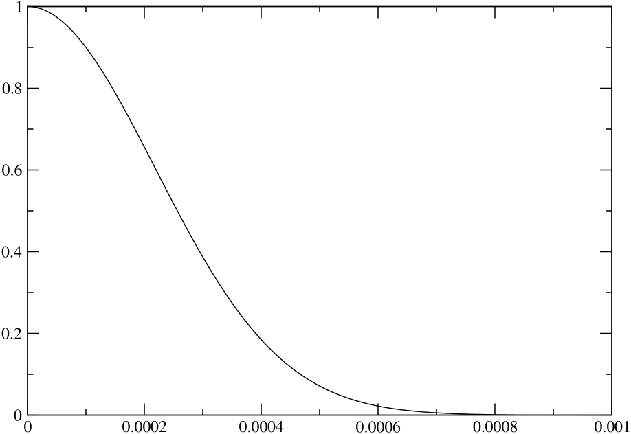
Figure 6: Figure 6: Evolution of $\Sigma^{nd}(t)$ for $M=10^{3}$ and $N=10^{2}$, with $t_{0}=1.10^{-3}s$.

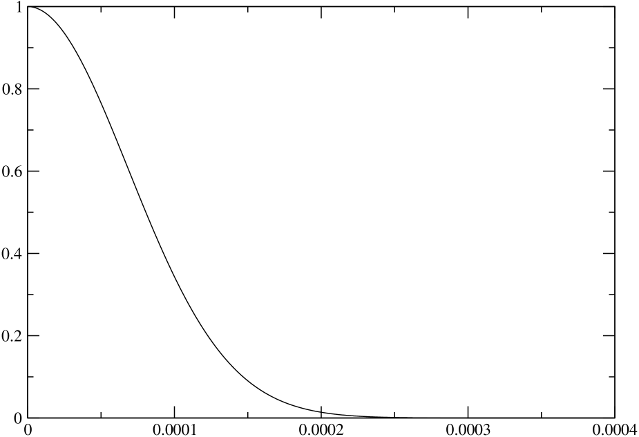
Figure 7: Figure 7: Evolution of $\Sigma^{nd}(t)$ for $M=10^{3}$ and $N=10^{3}$, with $t_{0}=4.10^{-4}s$.

Summarizing results

As we have seen, in this decomposition of the whole closed system, the open system $S=A_{M}$ decoheres when $N\gg 1$, independently of the value of $M$. But the particle $A_{M}$ was selected as $S$ only for computation simplicity: the same argument can be developed for any particle $A_{i}$ of $A$. Then, when $N\gg 1$ and independently of the value of $M$, any particle $A_{i}$ decoheres in interaction with its environment $E$ of $N+M-1$ particles.

On the other hand, as in Decomposition 1, here the symmetry of the whole system $U$ allows us to draw analogous conclusions when the system $S$ is one of the particles of $B$, say, $B_{N}$: $S=B_{N}$ decoheres when $M\gg 1$, independently of the value of $N$. And, on the basis of the same considerations as above, when $M\gg 1$ and independently of the value of $N$, any particle $B_{i}$ decoheres in interaction with its environment $E$ of $N+M-1$ particles.

VI Concluding remarks

In this paper we have studied a generalization of the spin-bath model, where a closed system $U$ is composed by two subsystems, $U=A\cup B$, with $A$ of $M$ particles $A_{i}$ and $B$ of $N$ particles $B_{i}$. We showed how the model behaves under different definitions of the system of interest and under different relations between the numbers $M$ and $N$.  The results so obtained allow us to state the following concluding remarks:

1. We have seen that, when $M\gg N$ or $M\simeq N$, the subsystem $A$ does not decohere (Decomposition 1 of Section IV), but the particles $A_{i}$, considered independently, decohere when $N\gg 1$ (Decomposition 2 of Section V). This means that there are physically meaningful situations, given by $M\gg N\gg 1$ or $M\simeq N\gg 1$, where all the $A_{i}$ decohere although $A$ does not decohere. In other words, in spite of the fact that certain particles decohere and may behave classically, the subsystem composed by all of them retains its quantum nature. We have also seen that, by symmetry, all the particles $B_{i}$, considered independently, also decohere when $M\gg 1$. Then, when $M\gg N\gg 1$ or $M\simeq N\gg 1$, the requirement $M\gg 1$ holds and we can conclude that not only all the $A_{i}$, but also all the $B_{i}$ decohere, although $B$ neither decoheres. So, all the particles of the closed system $U=$ $\left(\cup_{i}A_{i}\right)\cup\left(\cup_{j}B_{j}\right)$ may become classical when considered independently, although the whole system $U$ certainly does not decohere and, therefore, retains its quantum character. These results, considered together, are a clear manifestation of the fact, already pointed out by Schlosshauer (Schlosshauer ), that energy dissipation and decoherence are different phenomena: since all the particles of the system $U$ decohere when independently considered, decoherence cannot result from the dissipation of energy from the decohered systems to their environments.

2. The generalized model shows that the split of the entire closed system into an open system and its environment amounts to the selection of the observables relevant in each situation. Since there is no privileged or essential decomposition, we can select the observables of the subsystem $A$ in the situation in which $A$  does not decohere. In this way, it would be possible to use appropriately selected subsystems, unaffected by decoherence, for storing quantum information.

3. The natural further step of generalization will consist in following the ideas of paper Tessieri , and introducing coupling internal to the subsystems $A$ or $B$. For instance, given that the decoherence of $A$ is increasingly suppressed as the number $M$ of its particles increases, it could be expected that such decoherence suppression will also be more efficient as the interactions between the spins of the bath also increase.

References

- (1) W. H. Zurek, Phys. Rev. D, 26, 1862, 1982.
- (2) W. H. Zurek, Progr. Theor. Phys., 89, 281, 1993.
- (3) J. P. Paz and W. H. Zurek, “Environment-induced decoherence and the transition from quantum to classical”, in Dieter Heiss (ed.), Lecture Notes in Physics, Vol. 587, Heidelberg-Berlin: Springer, 2002.
- (4) W. H. Zurek, Rev. Mod. Phys., 75, 715, 2003.
- (5) S. Paganelli, F. de Pasquale and S. M. Giampaolo, Phys. Rev A, 66, 052317, 2002.
- (6) L. Tessieri and J. Wilkie, J. Phys. A: Math. Gen., 36, 12305, 2003.
- (7) C. M. Dawson et al., Phys. Rev A, 71, 052321, 2005.
- (8) F. M. Cucchietti, J. P. Paz, W. H. Zurek, Phys. Rev. A, 72, 052113, 2005.
- (9) H. T. Quan, Z. Song, X. F. Liu, P. Zanardi and C. P. Sun, Phys. Rev. Lett., 96, 140604, 2006.
- (10) D. Rossini et al., Phys. Rev. A, 75, 032333, 2007.
- (11) S. Camalet and R. Chitra, Phys. Rev. B, 75, 094434, 2007.
- (12) X. Z. Yuan, H-S Goan and K. D. Zhu, Phys. Rev. B, 75, 045331, 2007.
- (13) F. M. Cucchietti, S. Fernandez-Vidal and J. P. Paz, Phys. Rev. A, 75, 032337, 2007.
- (14) F. C. Lombardo and P. I. Villar, Int. J. Quantum Information, 6, 707, 2008.
- (15) M. Castagnino, S. Fortin, R. Laura and O. Lombardi, Class. Quant. Grav., 25, 154002, 2008.
- (16) M. Schlosshauer, Phys. Rev. A, 72, 012109, 2005.
- (17) M. Schlosshauer, Decoherence and the Quantum-to-Classical transition, Springer, Berlin, 2007.