Dispersion of biased swimming microorganisms in a fluid flowing through a tube

Abstract

Taylor dispersion, gyrotaxis, algae, bacteria, spermatozoa, swimming, Poiseuille flow, biofuel, photobioreactors Classical Taylor-Aris dispersion theory is extended to describe the transport of suspensions of self-propelled dipolar cells in a tubular flow. General expressions for the mean drift and effective diffusivity are determined exactly in terms of axial moments, and compared with an approximation a la Taylor. As in the Taylor-Aris case, the skewness of a finite distribution of biased swimming cells vanishes at long times. The general expressions can be applied to particular models of swimming microorganisms, and thus be used to predict swimming drift and diffusion in tubular bioreactors, and to elucidate competing unbounded swimming drift and diffusion descriptions. Here, specific examples are presented for gyrotactic swimming algae.

1 Introduction

Suspensions of swimming microorganisms, such as algae and bacteria, behave differently to molecular fluids. Many microorganisms exhibit taxes, directed motion relative to external or local cues. For example, various algae (e.g. Chlamydomonas and Dunaliella sp.) swim upwards on average in the dark (gravitaxis) due either to a centre-of-mass offset from the centre-of-buoyancy (Kessler 1986), sedimentation and anterior-posterior asymmetry in body/flagella (Roberts 2006), or active mechanisms (Häder et al.2005). This can result in aggregations of cells at upper boundaries and, if the cells are more dense than the medium in which they swim, overturning instabilities, termed bioconvection (Wager 1911; Platt 1961). Furthermore, a balance between gravitational and viscous torques can bias cells to swim towards downwelling regions, whence their added mass amplifies the downwelling. This is known as a gyrotactic instability and does not require an upper boundary. Of particular relevance here, Kessler (1986) observed that for a suspension of gyrotactic Chlamydomonas nivalis  in a vertically aligned tube, cells became sharply focused at the centre for downwelling flow and scattered towards the edges when the flow was upwelling. Additionally, phototrophic algae are often phototactic (they swim towards weak light and away from bright light), which can modify the instability mechanisms above, and bacteria may exhibit chemotaxis (e.g. up oxygen gradients). In shallow containers, the above taxes can result in very distinct bioconvection patterns, with characteristic lengthscales of millimeters to centimetres in just tens of seconds (Bees & Hill 1997). See Pedley & Kessler (1992) and Hill & Pedley (2005) for reviews. In deep cultures, one may observe long thin plumes of cells (Figure 1) that have a clear impact on the transmittance of light through the culture, of some relevance to photosynthetic algae (a “Cheese plant effect”).

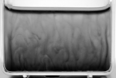
a)    b) 

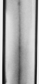
Figure 1: Bioconvection plumes in suspensions of C. nivalis  in a) a culture flask (5.3 cm wide), and b) a long vertical tube of inner diameter 1.1 cm. Concentration $\approx 1.5\times 10^{6}$ cm^-3.

Recently there has been renewed interest in utilizing microorganisms for fuel production. For green algae there are two main approaches: hydrogen production by sulphur deficient cells (Melis & Happe 2002) and biomass generation for biodiesel production (Chisti 2007). To reach economical viability, both methods require the sustainable culture of cells, extensively and under carefully controlled conditions. Culture systems typically consist of arrays of tubes (vertical, horizontal or helical) and aim to maximize light whilst maintaining linear separation of cell stage and medium victuals. In algal bioreactors, suspensions of algae are typically pumped and may be bubbled or tansported turbulently to enhance nutrient/gas mixing and reduce variance in light exposure. These processes, which treat a suspension of microorganisms like a chemical fluid, are energetically costly. Instead, efficient bioreactor designs might hope to harness the activity of the swimming microorganisms directly in laminar flows. However, it is unclear how a) the mean cell drift and b) the effective axial swimming dispersion of cells are affected by various flow fields in the aforementioned tube arrangements.

In a series of papers Taylor (1953, 1954a, 1954b) described how it is possible to approximate the effective axial diffusion of a solute in a fluid flowing through a tube. Molecular diffusion and advection by shear each play a distinguished role, such that the effective diffusivity is given by $D_{m}+U^{2}a^{2}/48D_{m}$, where $D_{m}$ is the molecular diffusivity, $a$ is the radius of the tube and $U$ is the mean flow speed. Subsequently, Aris (1955) formalized the approach by solving the moment equations, extending ubiquitously the domain of physical relevance of Taylor’s result. The methods have been extended by many authors (e.g. Horn & Kipp 1971, partitioning reactions between phases; Brenner 1980, dispersion in periodic porous media). The value of the Taylor-Aris approach can be measured by the wealth of practical applications (see Alizadeh et al.1980). Until now, the approach has not been extended to suspensions of biased swimming microorganisms in a tubular flow. As we shall see, it is possible to derive general expressions with few assumptions. However, these expressions depend upon constitutive equations for the mean behaviour of the cells.

We shall adopt the standard continuum approach to modelling bioconvective phenomena, although our main result is independent of the details of these descriptions. Recent models of dilute, gyrotactic bioconvection (Childress et al.1975; Pedley & Kessler 1990, 1992) assume that the fluid flow is governed by the Navier-Stokes equations with a negative buoyancy term to represent the effect of the cells on the fluid (Boussinesq approximation) such that

$$\rho\frac{D{\bf u}}{Dt}=-\nabla p_{e}+nv\Delta\rho{\bf g}+\nabla\cdot\mathbf{\Sigma},$$ (1)

where ${\bf u}({\bf x},t)$ is the velocity of the suspension, $p_{e}({\bf x},t)$ is the excess pressure, $\mathbf{\Sigma}({\bf x},t)$ is the stress tensor, ${\bf g}$ is the acceleration due to gravity, $n({\bf x},t)$ is the cell concentration, $\Delta\rho$ is the difference between the cell and fluid density, $\rho$, and $v$ is the mean volume of a cell. The cell Reynolds number is small (e.g. $\sim 10^{-3}$ for C. nivalis). Furthermore, the suspension is assumed incompressible such that $\nabla\cdot{\bf u}=0$. Pedley & Kessler (1990) extended the standard Newtonian description to include Batchelor stresses, stress associated with rotary particle diffusion, and swimming induced stresslets. The first two were found to be qualitatively and quantitatively insignificant, and the third only plays a role in concentrated regions of the suspension. Thus in a dilute limit one may write $\nabla\cdot\mathbf{\Sigma}=\mu\nabla^{2}{\bf u}$, where $\mu$ is the fluid viscosity. We shall employ this approximation in explicit examples, but the main result does not require it. Typically, over the course of a bioconvection experiment the total number of cells is conserved, so that one may write

$$\frac{\partial n}{\partial t}=-\nabla\cdot\left[n\left({\bf u}+{\bf V}_{c}\right)-{\bf D}\cdot\nabla n\right],$$ (2)

where ${\bf V}_{c}({\bf x})$ is the mean cell swimming velocity and ${\bf D}({\bf x})$ is the cell swimming diffusion tensor, both of which need to be determined. At rigid boundaries, ${\cal G}$, we require a no-slip condition, ${\bf u}={\bf 0}\mbox{~{}on~{}}{\cal G},$ as well as zero cell flux normal to ${\cal G}$ (in direction ${\bf n}$), such that ${\bf n}\cdot\left(n\left({\bf u}+{\bf V}_{c}\right)-{\bf D}\cdot\nabla n\right)=0\mbox{~{}on~{}}{\cal G}.$

To model gyrotaxis, Pedley & Kessler (1987) employed a deterministic balance of gravitational and viscous torques on a spheroidal cell, of eccentricity $\alpha_{0}$, to determine the cell orientation ${\bf p}$:

$$\dot{{\bf p}}=\frac{1}{2B}\left[{\bf k}-({\bf k}\cdot{\bf p}){\bf p}\right]+\frac{1}{2}\mathbf{\Omega}{\wedge}{\bf p}+\alpha_{0}{\bf p}\cdot{\bf E}\cdot({\bf I}-{\bf p}{\bf p}).$$ (3)

Here, $B$ is the gyrotactic reorientation time-scale of a cell affected by external (gravitational) torques subject to resisting viscous torques, given by $B={\mu\alpha_{\perp}}/{2h\rho g}$, where $h$ is the centre-of-mass offset relative to the centre-of-buoyancy and $\alpha_{\perp}$ is the dimensionless resistance coefficient for rotation about an axis perpendicular to ${\bf p}$. $\mathbf{\Omega}$ and ${\bf E}$ are the local vorticity vector and rate-of-strain tensor, respectively. These authors then wrote ${\bf V}_{c}=V_{s}{\bf p}$, where $V_{s}$ is the mean swimming speed, and, as for earlier models, assumed a constant isotropic diffusion. Pedley & Kessler (1990) advanced this description by postulating that the probability density function, $f({\bf p},t)$, for orientation ${\bf p}$ satisfies a Fokker-Planck equation, with drift due to the various torques and a rotational diffusivity analogous to rotational Brownian motion (Frankel & Brenner 1991), thus taking account of biological variation of swimming stroke. Experimental data on cell tracking (Hill & Häder 1997) has provided values for the deterministic and diffusive parameters. From $f({\bf p})$, the mean swimming direction, ${\bf q}$, is easily calculated, yielding ${\bf V}_{c}=V_{s}{\bf q}$, but the cell swimming diffusion tensor is not and requires approximation. Pedley & Kessler (1990) suggested that ${\bf D}\approx V_{s}^{2}\tau\mbox{var}({\bf p})$, where $\tau$ is a direction correlation time, estimated from experimental data, and found asymptotic solutions for small flow gradients. Bees et al.(1998) extended these solutions for all flow gradients by expansion in spherical harmonics (employed in Bees & Hill 1998, 1999). However, the ad hoc nature of the diffusion approximation was cause for concern. This motivated Hill & Bees (2002) and Manela & Frankel (2003) to develop generalized Taylor dispersion theory (Frankel & Brenner 1991), taking account of both the orientation and position of cells swimming in a linear flow, to derive the leading order, long time, spatial diffusion tensor. The techniques were subsequently employed by Bearon (2003) for dispersion of chemotactic bacteria in a shear flow.

There are significant qualitative differences between the three treatments described above as vorticity is varied. In particular, as vorticity, $\mathbf{\omega}$, is increased the Fokker-Planck and the generalized Taylor dispersion approaches provide eigenvalues of the diffusion tensor that tend towards non-zero and zero limits, respectively. This is due to the fundamental difference between the orientation only versus trajectory based descriptions. Such qualitative differences in behaviour need to be tested with laboratory experiments. One approach is to track individual microorganisms in the very dilute limit (Hill & Häder 1997; Vladimirov et al.2004) but for a precisely prescribed shear flow (e.g. Durham et al.2009). However, such a scheme would likely be laborious and may not easily yield significant results for large shear rates. A macroscopic approach would be much preferred. In general, the coupling between cell and fluid is bidirectional; the flow is driven by the presence of the cells, which determines the swimming directions of the cells. Controlling the flow in the manner described by Taylor may thus be advantageous. There are, however, some obstacles to be overcome. In particular, a local distribution of cells will drive secondary flows and lead to an effective axial diffusivity that depends on the axial location. The answer is to create a flow that is independent of the presence of the cells. This can be achieved by creating a long axisymmetric plume of swimming cells and dying a small blob of cells within the plume (Figure 2). In this way, we partially uncouple the drift-diffusive dynamics of the dyed cells from the bulk flow-cell problem.

In the next section, we shall describe the geometry and scaling of the problem and introduce the method of moments. In section 3, steady-state solutions of plume concentration and flow in a tube subject to a pressure gradient are calculated. In section 4, the long-term drift and effective diffusion of a blob of cells in a plume in a tube of circular cross-section are formulated in general terms. The skewness of the distribution is also determined. For general comprehension and comparison, an argument in a vein similar to that given by Taylor (1953) is presented in section 5. The full theoretical results are then summarized in section 6 before explicit example calculations are given. Conclusions are presented in section 7.

2 Flow in a straight tube

This analysis is applicable to the case where the flow is independent of the axial direction. Thus consider the diffusion of dyed cells within a long plume.

We follow the notation of Aris (1955) and consider a tube with characteristic scale $a$ with axis parallel to the vertical $x$-axis (pointing in the downwards direction; see Figure 2). The interior of the tube is denoted by $S$, its cross-sectional area by $s$ and its perimeter by $\Gamma$. We consider flows, ${\bf u}$, generated by a pressure gradient and the added mass of the algae such that

$${\bf u}({\bf x}_{H})=u({\bf x}_{H}){\bf e}_{x}=U[1+\chi({\bf x}_{H})]{\bf e}_{x},$$ (4)

where $U$ is the mean flow speed and $\chi$ is the flow speed relative to the mean and is assumed to be only a function of the cross-sectional coordinates ${\bf x}_{H}$. Clearly, a no-slip boundary condition provides $\chi=-1$ on $\Gamma$.

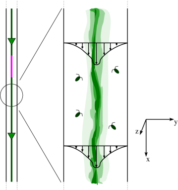
Figure 2: Tube arrangement and coordinates. The magenta (light grey) region on the left represents dyed cells for which drift and diffusion is to be calculated.

Let the cell swimming diffusion tensor be of the form $D^{c}{\bf D}$, where $D^{c}$ is its characteristic scale, and the mean cell swimming velocity be $V_{s}{\bf q}({\bf x}_{H})$ (see Bees et al.1998, where ${\bf q}\equiv\langle{\bf p}\rangle$), where $V_{s}$ is the mean swimming speed. As $\chi$ is independent of the axial direction then so are ${\bf D}$ and ${\bf q}$. This fact permits a treatment using the method of moments in a similar vein to that described in Aris (1955).

The cell conservation equation (2) can thus be written

$$\frac{1}{D^{c}}n_{t}=\nabla\cdot\left({\bf D}\cdot\nabla n\right)-\frac{U}{D^{c}}\left(1+\chi\right)n_{x}-\frac{V_{s}}{D^{c}}\nabla\cdot\left(n{\bf q}\right),$$ (5)

where we use subscripts for partial differentiation where it is clear. It is conducive to translate to a reference frame travelling with the mean flow, and non-dimensionalize, such that $\hat{x}=(x-Ut)/a$, $\hat{{\bf x}}_{H}={\bf x}_{H}/a$ and $\hat{t}=D^{c}t/a^{2}$. Equation (5) becomes

$$n_{t}=\nabla\cdot\left({\bf D}\cdot\nabla n\right)-\mbox{Pe}\chi n_{x}-\beta\nabla\cdot\left(n{\bf q}\right),$$ (6)

where

$$\mbox{Pe}=\frac{Ua}{D^{c}},\mbox{~{}~{}~{}~{}and~{}~{}~{}~{}}\beta=\frac{V_{s}a}{D^{c}}\left(=\frac{a}{V_{s}\tau}\right),$$ (7)

and the hats are dropped for notational clarity. Here, Pe is a Peclet number, which is a ratio of the rate of advection by the flow to the rate of swimming diffusion, and $\beta$ is a ‘swimming’ Peclet number, a ratio of the rates of transport by swimming to swimming diffusion (or tube radius to swimming correlation length, where $\tau$ is the direction correlation time, as typically $D^{c}=V_{s}^{2}\tau$; e.g. Pedley & Kessler 1990). No-flow and no-flux boundary conditions shall be applied to the solution, such that

$${\bf u}={\bf 0}\mbox{~{}~{}~{}~{}and~{}~{}~{}~{}}{\bf n}\cdot\left({\bf D}\cdot\nabla n-\beta{\bf q}n\right)=0,\mbox{~{}~{}~{}~{}on~{}~{}~{}~{}}\Gamma,$$ (8)

respectively, where ${\bf n}$ is normal to $\Gamma$.

The $p$th moment with respect to the axial direction through ${\bf x}_{H}$ is defined as

$$c_{p}({\bf x}_{H},t)=\int^{+\infty}_{-\infty}x^{p}n(x,{\bf x}_{H},t)dx,$$ (9)

provided it exists and is finite (i.e. $x^{p}n(x,{\bf x}_{H},t)\to 0$ as $x\to\pm\infty$). The cross-sectional average (denoted by an overbar) of this moment is written

$$m_{p}(t)=\overline{c_{p}}=\frac{1}{s}\int\int_{S}c_{p}dS.$$ (10)

Henceforth, consider axisymmetric flows in a tube of circular cross-section with radius $a$ oriented parallel to the vertical $x$-axis (pointing downwards). Here $\chi=\chi(r)$, ${\bf D}={\bf D}(r)$ and ${\bf q}={\bf q}(r)$ (such that ${\bf q}$ has no component in the ${\bf e}_{\theta}$ direction).

In cylindrical coordinates, by multiplying by $x^{p}$ and integrating over the length of an infinite pipe, equation (6) becomes

$$c_{p,t} = \frac{1}{r}\left[r(D^{rr}c_{p,r}-\beta q^{r}c_{p}-pD^{rx}c_{p-1})\right]_{r}-pD^{rx}c_{p-1,r}$$ (11)

$$+p(\mbox{Pe}\,\chi+\beta q^{x})c_{p-1}+p(p-1)D^{xx}c_{p-2},$$

with

$$D^{rr}c_{p,r}-\beta q^{r}c_{p}-pD^{rx}c_{p-1}=0\mbox{~{}~{}~{}~{}on~{}~{}~{}~{}}r=1.$$ (12)

Averaging over the cross-section (applying no-flux boundary conditions 12) yields

$$m_{p,t}=-p\overline{D^{rx}c_{p-1,r}}+p\overline{\left(\mbox{Pe}\chi+\beta q^{x}\right)c_{p-1}}+p(p-1)\overline{D^{xx}c_{p-2}}.$$ (13)

Before deriving results for drift and diffusion in section 4, we shall solve the steady, coupled, cell conservation and hydrodynamic problem.

3 Steady problem: flow and cell concentration

Kessler (1986) demonstrated theoretically and experimentally that plume solutions exist in vertically aligned tubes. He found that the plumes are generally stable when a pressure gradient is applied such that the flow is downwards. However, varicose instabilities may arise when no pressure gradient is applied. Here, we aim to avoid such instabilities and thus in the ensuing analysis implicitly refer to parameter regimes where plume solutions are stable.

In later sections, in order to compute the dispersion of a blob of cells within a plume, we require knowledge of $\chi$, the fluid velocity relative to the mean. Hence, when $\chi(r)$ represents the steady fluid velocity induced by a pressure gradient and the presence of a swimming cell distribution that is independent of $x$,

$$0=\nabla\cdot\left({\bf D}\cdot\nabla n^{*}\right)-\beta\nabla\cdot\left({\bf q}n^{*}\right)$$ (14)

where $n^{*}$ now represents all cells in the plume, and not just those dyed cells for which we shall calculate dispersion. As $n^{*}_{r}=0=q^{r}$ at $r=0$, this implies that

$$D^{rr}n^{*}_{r}=\beta q^{r}n^{*}.$$ (15)

Hence, given $D^{rr}(r)$ and $q^{r}(r)$ we have

$$\tilde{n}=\tilde{n}(0)\exp{\left(\beta\int^{r}_{0}\frac{q^{r}(s)}{D^{rr}(s)}ds\right)},$$ (16)

where $\tilde{n}$ is non-dimensional cell concentration (scaled with the average concentration, $\overline{n^{*}}$). Note, for a spherical cell ($\alpha_{0}=0$), $q^{r}$ and $D^{rr}$ are functions of vorticity only, which must be in the ${\bf e}_{\theta}$ direction: $\mathbf{\omega}=\nabla{\wedge}{\bf u}=-\chi_{r}(r){\bf e}_{\theta}=\mathbf{\omega}{\bf e}_{\theta}$.

In cylindrical polars the steady flow equation (1) in the dilute limit becomes

$$\nabla^{2}\frac{u}{U}=\frac{1}{r}\left(r\chi_{r}\right)_{r}=\tilde{p}_{x}-\alpha\tilde{n},$$ (17)

subject to the boundary conditions $\chi_{r}(0)=0$ and $\chi(1)=-1.$ Here, the non-dimensional pressure gradient is $\tilde{p}_{x}=p_{x}a/U\mu$, and

$$\alpha=\frac{a^{2}vg\Delta\rho N}{U\nu\rho},$$ (18)

measures the magnitude of the effect that the cells have on the flow. $g$ is the acceleration due to gravity acting in the positive $x$-direction.

Contrary to intuition, $\tilde{p}_{x}$ and $\alpha$ are not free parameters but are linked to the mean flow speed, $U$, introduced in equation (4). Together they are determined by the boundary conditions on $\chi$ and the requirement that $\bar{\chi}=0$; the flow deviation relative to the mean is order one. For Poiseuille flow, where $\alpha=0$, it is well known that $\tilde{p}_{x}=-8$, such that $\chi=1-2r^{2}$.

Substituting (16) for $\tilde{n}$, equation (17) can be rewritten as

$$\frac{1}{r}\left(r\chi_{r}\right)_{r}-\tilde{p}_{x}=-\alpha\,\tilde{n}(0)\exp{\left(\beta\int_{0}^{r}\frac{q^{r}(s)}{D^{rr}(s)}ds\right)}.$$ (19)

For spherical cells ($\alpha_{0}=0$), taking logs and differentiating provides

$$\frac{\left(\frac{1}{r}\left(r\chi_{r}\right)_{r}\right)_{r}}{\frac{1}{r}\left(r\chi_{r}\right)_{r}-\tilde{p}_{x}}=\beta\frac{q^{r}(\omega)}{D^{rr}(\omega)}=:\gamma(\omega).$$ (20)

Note, differentiating removes the dependence on $\alpha$; to fully specify the constants of integration, substitution back into Equation (19) will be required. In general, equation (20) can be solved for $\omega$ and, thus, $\chi$ and $\tilde{n}$ (with application of the boundary conditions). Later, we shall consider the simple case $\gamma(\omega)\approx A\omega$, for constant and negative $A$, so here we derive expressions for $\chi$ in this limit. Equation (20) becomes

$$r^{2}\omega^{\prime\prime}+\left(r-A\omega r^{2}\right)\omega^{\prime}-\left(1+rA\omega)\right)\omega=\tilde{p}_{x}r^{2}A\omega.$$ (21)

$r=0$ is a singular point and so consider $\omega=\sum^{\infty}_{m=0}b_{m}r^{m+Q}$, where constant $Q$ is to be determined. Substituting into the nonlinear equation and examining coefficients reveals $Q=1$, for finite solutions at $r=0$. Furthermore, the recurrence relation

$$b_{t}=\frac{A\left[\tilde{p}_{x}b_{t-2}+\sum^{t-2}_{m=0}b_{m}b_{t-m-2}(m+2)\right]}{t(t+2)},$$ (22)

is forthcoming. We require that $\omega$ is odd and, therefore, $b_{i}=0$, $\forall i$ odd. Hence, the first few coefficients are given by

$$b_{2}=\frac{Ab_{0}}{2^{3}}[\tilde{p}_{x}+2b_{0}],\mbox{~{}~{}~{}~{}}b_{4}=\frac{A^{2}b_{0}}{2^{6}3}[\tilde{p}_{x}+2b_{0}][\tilde{p}_{x}+6b_{0}],$$

$$b_{6}=\frac{A^{3}b_{0}}{2^{10}3^{2}}[\tilde{p}_{x}+2b_{0}][\tilde{p}_{x}+6b_{0}][\tilde{p}_{x}+8b_{0}]+\frac{A^{3}b_{0}^{2}}{2^{8}3}[\tilde{p}_{x}+2b_{0}]^{2}.$$ (23)

Furthermore, application of the boundary conditions yields

$$\chi=-1+\sum^{\infty}_{m=0}\frac{b_{m}}{m+2}(1-r^{m+2}).$$ (24)

Applying the condition $\overline{\chi}=0$ admits the result

$$b_{0}=4\left(1-\sum_{m=1}^{\infty}\frac{b_{m}}{m+4}\right).$$ (25)

Finally, substitution of $\chi$ into Equation (19) is required to find $\alpha$ in terms of $b_{m}$, $m=0,2,4,...$, and $\tilde{p}_{x}$. Equation (19) can be written

$$\left(r\chi_{r}\right)_{r}-r\tilde{p}_{x}=-r\tilde{\alpha}\exp{\left[-A\chi(r)\right]},$$ (26)

where $\tilde{\alpha}=\alpha\tilde{n}(0)\exp{(A\chi(0))}$ (evaluated with the normalization condition $\overline{\tilde{n}}=1$, giving $\tilde{n}(0)e^{A\chi(0)}=1/{2\int_{0}^{1}e^{-A\chi(r)}r\,dr}$). Hence, substituting $\chi$ into (26) and comparing coefficients at leading order in $r$ we find that

$$\tilde{\alpha}=\left[2b_{0}+\tilde{p}_{x}\right]\exp\left\{-A\left(1-\sum_{m=0}^{\infty}\frac{b_{m}}{m+2}\right)\right\}.$$ (27)

Higher orders in $r$ provide a check for the previously computed $b_{m}$, $m=2,4,6,...$. Therefore, given $b_{m}$, $m=0,2,4,...$, and $\tilde{p}_{x}$, then $\tilde{\alpha}$ can be computed from (27).

If $b_{0}=b_{0}(\tilde{\alpha})$ is required, and in the particular case that $A$ is small (i.e. the cells are weakly affected by the flow; e.g. $B$ is small), such that we can neglect quadratic terms in $A$ and higher, then we can expand the transcendental equation to give

$$b_{0}=\frac{-2\tilde{p}_{x}+2\tilde{\alpha}\left\{1+A\left(1-\sum_{m=1}^{\infty}\frac{b_{m}}{m+2}\right)\right\}}{4+\tilde{\alpha}A}.$$ (28)

Three examples are presented below, with the profiles plotted in Figure 3.

• One of the simplest cases is for $\tilde{\alpha}=0$ (i.e. the presence of the cells does not affect the flow). In this case, we compute $b_{0}=-\tilde{p}_{x}/2$ and $b_{m}=0$, $m=2,4,6,...$, such that $\chi=-1+\tilde{p}_{x}(r^{2}-1)/4$, which is Poiseuille flow. Equation (25) gives $b_{0}=4=-\tilde{p}_{x}/2$, as would be expected.

• With $\tilde{\alpha}\neq 0$ and $A<0$ small (i.e. a broad plume), but a zero pressure gradient, $\tilde{p}_{x}=0$, then $b_{2}=Ab_{0}^{2}/4$, $b_{m}=O(A^{2})$, $m=4,6,8,...$. and equations (25) and (28) provide $b_{0}=6(-1\pm\sqrt{1+8A/3})/2A+O(A^{2})=\tilde{\alpha}\left[1+\left(1-\tilde{\alpha}/4\right)A\right]+O(A^{2})$. Thus $\chi=-1+b_{0}(1-r^{2})/2+Ab_{0}^{2}(1-r^{4})/16+O(A^{2})$. Two solutions are possible: a simple positive flow (mode 1), and one with upwelling towards the edge of the tube (mode 2). For zero pressure gradient, a closed form, mode 1 solution is known. Kessler (1986) noted that $\tilde{n}=\tilde{n}(0)/(1+C_{1}\tilde{n}(0)r^{2})^{2}$ is a solution, for constant $C_{1}$. Applying the condition $\overline{\tilde{n}}=1$ gives $C_{1}=\tilde{n}(0)-1$. Substituting this solution back into the governing equation reveals that $\tilde{n}(0)$ is determined by the constrained parameter $\tilde{\alpha}$, as should be the case, in the same way that the mean velocity is linked to the pressure gradient in Poiseuille flow. This closed-form profile is approached by the above mode 1 profile with truncated sums (not shown).

• The case $A<0$ (small; a broad plume) and $\tilde{p}_{x}\neq 0$ is also of interest, and has not previously been investigated. If $A=-\frac{1}{4}$ and $\tilde{p}_{x}=-6$, then we calculate $b_{2}=-b_{0}(b_{0}-3)/2^{4}$, $b_{4}=b_{0}(b_{0}-3)(b_{0}-1)/2^{8}$, and $b_{6}=-b_{0}(b_{0}-3)(b_{0}-1)(4b_{0}-3)/(2^{13}3)-b_{0}^{2}(b_{0}-3)^{2}/(2^{12}3)$. From equation (25) we compute the two solutions $b_{0}\approx 4.179$ and $21.931$. Again, the mode 2 solution corresponds to a flow with upwelling near the edge of the tube. The corresponding $\tilde{\alpha}$ can be evaluated from equation (27). Hence, for the mode 1 solution, $\chi=-1+4.179(1-r^{2})/2-0.308(1-r^{4})/4+0.0612(1-r^{6})/6-0.0107(1-r^{8})/8+...$.

Figure 3: Flow profiles for three cases (see text; extended to cover the width of the tube): $\tilde{\alpha}=0$, $\tilde{p}_{x}=-8$ (solid); $\tilde{\alpha}\neq 0$, $\tilde{p}_{x}=0$, $A=-\frac{1}{4}$ (two dashed curves); $\tilde{\alpha}\neq 0$, $\tilde{p}_{x}=-6$, $A=-\frac{1}{4}$ (dotted and dot-dashed curves). Selected broad cell distributions, $\tilde{n}/\tilde{n}(0)e^{\chi(0)}$, are also plotted (inset; see text).

4 Dispersion in a tube of circular cross-section

In this section, we place no restrictions on the cell shape (e.g. spheroidal cells) and form of $\chi(r)$, ${\bf q}(r)$ and ${\bf D}(r)$, and find general expressions for the drift and effective diffusion of a blob of dyed cells within an existing plume.

4.1 Cell conservation and drift

For $p=0$ equation (13) gives $m_{0,t}=0$, so that $m_{0}$ is a constant (i.e. number of cells is conserved). We fix $m_{0}=1$ (and remember that these cells represent dyed cells diffusing within a plume of other cells). Equation (11) with $p=0$ implies that

$$c_{0,t}=\frac{1}{r}\left[r(D^{rr}c_{0,r}-\beta q^{r}c_{0})\right]_{r},$$ (29)

with boundary condition $D^{rr}c_{0,r}-\beta q^{r}c_{0}=0$ on $r=1$. The solution takes the form

$$c_{0}=R_{0}^{0}(r)+\sum^{\infty}_{n=1}R_{n}^{0}(r)T_{n}^{0}(t),$$ (30)

where $T_{n}^{0}=\exp{\left(-\gamma_{n}^{2}t\right)}$ and $R_{n}^{0}$ satisfies

$$rD^{rr}R_{n}^{0\prime\prime}+\left(D^{rr}+rD^{rr\prime}\right)R_{n}^{0\prime}+\left(-\beta q^{r}-r\beta q^{r\prime}+\gamma_{n}^{2}r\right)R_{n}^{0}=0,$$ (31)

subject to the initial conditions. The solution for $R_{0}^{0}$, such that $\overline{R_{0}^{0}}(=\overline{c_{0}})=1$, is

$$R_{0}^{0}(r)=\exp{\left(\beta\int^{r}_{0}\frac{q^{r}(s)}{D^{rr}(s)}ds\right)}\left\{\overline{\exp{\left(\beta\int^{r}_{0}\frac{q^{r}(s)}{D^{rr}(s)}ds\right)}}\right\}^{-1}.$$ (32)

Note also that $\overline{R_{n}^{0}}=0$, $n\neq 0$. Putting $p=1$ in (13) gives

$$m_{1,t}=\Lambda_{0}+\sum_{n=1}^{\infty}\exp{\left(-\gamma_{n}^{2}t\right)}\Lambda_{n},\mbox{~{}~{}~{}where~{}~{}~{}}\Lambda_{n}=-\overline{D^{rx}R_{n}^{0\prime}}+\overline{\left(\mbox{Pe}\chi+\beta q^{x}\right)R_{n}^{0}}.$$ (33)

In particular, it is clear that

$$\lim_{t\rightarrow\infty}m_{1,t}=\Lambda_{0}=-\overline{D^{rx}R_{0}^{0\prime}}+\overline{\left(\mbox{Pe}\chi+\beta q^{x}\right)R_{0}^{0}}.$$ (34)

This means that the mean of the blob of dyed cells will move at a speed of $\Lambda_{0}$ relative to the mean flow. Hence,

$$m_{1}(t)=\Lambda_{0}t+\sum_{n=1}^{\infty}\frac{1}{\gamma_{n}^{2}}\left(1-\exp{\left(-\gamma_{n}^{2}t\right)}\right)\Lambda_{n},$$ (35)

where we have used $m_{10}=0$. The first term of $\Lambda_{0}$ in (34) is associated with a diffusive flux, the second with advection of the cells heterogeneously distributed near the axis of the tube, and the third to swimming in the vertical direction relative to the fluid motion. At long times we expect

$$m_{1\infty}(t)=\Lambda_{0}t+\sum_{n=1}^{\infty}\frac{\Lambda_{n}}{\gamma_{n}^{2}},$$ (36)

4.2 Effective diffusion

With $p=1$, equation (11) implies that

$$c_{1,t}-\frac{1}{r}\left[r(D^{rr}c_{1,r}-\beta q^{r}c_{1}-D^{rx}c_{0})\right]_{r}=-D^{rx}c_{0,r}+(\mbox{Pe}\,\chi+\beta q^{x})c_{0},$$ (37)

with boundary condition

$$D^{rr}c_{1,r}-\beta q^{r}c_{1}-D^{rx}c_{0}=0\mbox{~{}~{}~{}~{}on~{}~{}~{}~{}}r=1.$$ (38)

The solution of this equation can be constructed in three parts.

1. Particular integral from $R_{0}^{0}(r)$ in $c_{0}$. It satisfies

   $$-c_{1,t}^{1}+\frac{1}{r}\left[r\left(D^{rr}c^{1}_{1,r}-\beta q^{r}c^{1}_{1}-D^{rx}R_{0}^{0}\right)\right]_{r}=D^{rx}{R_{0}^{0}}^{\prime}-\left(\mbox{Pe}\chi+\beta q^{x}\right)R_{0}^{0}.$$ (39)

2. Particular integral from the rest of the terms $R_{n}^{0}(r)\exp{(-\gamma_{n}^{2}t)}$, $n\neq 0$, in $c_{0}$.

   $$-c_{1,t}^{2}+\frac{1}{r}\left[r\left(D^{rr}c^{2}_{1,r}-\beta q^{r}c^{2}_{1}-D^{rx}R_{n}^{0}(r)e^{-\gamma_{n}^{2}t}\right)\right]_{r}$$

   $$=D^{rx}{R_{n}^{0}(r)}^{\prime}e^{-\gamma_{n}^{2}t}-\left(\mbox{Pe}\chi+\beta q^{x}\right)R_{n}^{0}(r)e^{-\gamma_{n}^{2}t}.$$ (40)

   It is quite clear that solutions to (40) are of the form $S_{n}(r)\exp{(-\gamma_{n}^{2}t)}$, where $S_{n}$ satisfy no-flux boundary conditions and are found by solving

   $$\gamma_{n}^{2}S_{n}(r)+\frac{1}{r}\left[r\left(D^{rr}S_{n}(r)^{\prime}-\beta q^{r}S(r)-D^{rx}R_{n}^{0}(r)\right)\right]_{r}$$

   $$=D^{rx}{R_{n}^{0}(r)}^{\prime}-\left(\mbox{Pe}\chi+\beta q^{x}\right)R_{n}^{0}(r).$$ (41)

   As we are interested in long-time behaviour, we do not solve for $S_{n}(r)$, but later will require its cross-sectional average. This can be found by averaging both sides of (41) and using the boundary conditions (38), to give

   $$\overline{S_{n}}=-\frac{1}{\gamma_{n}^{2}}\left[-\overline{D^{rx}{R_{n}^{0}}^{\prime}}+\overline{\left(\mbox{Pe}\chi+\beta q^{x}\right)R_{n}^{0}}\right]=-\frac{\Lambda_{n}}{\gamma_{n}^{2}}.$$ (42)

3. Complementary function. Solutions of (37) without terms in $c_{0}$ that satisfy (38) are of the form $A^{1}_{n}R_{n}^{0}(r)e^{-\gamma_{n}^{2}t},$ where $A_{n}^{1}$ are constants.

For item 1, to calculate $c_{1}^{1}$, we rewrite the equation as

$$c_{1,t}^{1}r-\left[r\left(D^{rr}c^{1}_{1,r}-\beta q^{r}c^{1}_{1}-D^{rx}R_{0}^{0}\right)\right]_{r}=r\left(-D^{rx}{R_{0}^{0}}^{\prime}+\left(\mbox{Pe}\chi+\beta q^{x}\right)R^{0}_{0}\right)=:\lambda_{0}(r),$$ (43)

Recalling that $R_{0}^{0}$ satisfies $D^{rr}{R_{0}^{0}}^{\prime}-\beta q^{r}R_{0}^{0}=0$, let $c^{1}_{1}(r,t)=\left[Mt+f(r)\right]R^{0}_{0}$, where $M$ is a constant and $f(r)$ is a function of $r$. Then, (43) becomes

$$\left[r(f^{\prime}D^{rr}R_{0}^{0}-D^{rx}R^{0}_{0})\right]^{\prime}=-\lambda_{0}+MR^{0}_{0}r,$$ (44)

an equation independent of $t$. Hence, integrating once provides

$$r(f^{\prime}D^{rr}R_{0}^{0}-D^{rx}R^{0}_{0})=-\frac{1}{2}\Lambda_{0}^{*}(r)+\frac{1}{2}Mm^{*}_{0}(r),$$ (45)

where

$$\Lambda_{0}^{*}(r)=2\int^{r}_{0}\lambda_{0}(s)ds=2\int^{r}_{0}s\left(-D^{rx}{R_{0}^{0}}^{\prime}+\left(\mbox{Pe}\chi+\beta q^{x}\right)R^{0}_{0}\right)ds,$$ (46)

$$m_{0}^{*}(r)=2\int^{r}_{0}sR^{0}_{0}(s)ds,$$ (47)

$\Lambda_{0}^{*}(1)=\Lambda_{0}$ and $m_{0}^{*}(1)=1$. Applying the no-flux boundary condition (38) to (45) yields $M=\Lambda_{0}$. Integrating (45) again provides

$$c_{1}^{1}(r,t)=R_{0}^{0}(r)\left(\Lambda_{0}t+f(r)\right)=\left[\Lambda_{0}t+J(r)-\Phi(r)\right]R^{0}_{0}(r),$$ (48)

where

$$J(r)=\int^{r}_{0}\frac{D^{rx}(s)}{D^{rr}(s)}ds\mbox{~{}~{}~{}~{}and~{}~{}~{}~{}}\Phi(r)=\frac{1}{2}\int^{r}_{0}\left(\frac{\Lambda_{0}^{*}(s)-\Lambda_{0}m_{0}^{*}(s)}{sD^{rr}(s)R^{0}_{0}(s)}\right)ds.$$ (49)

Hence, the complete solution $c_{1}=c^{1}_{1}+c^{2}_{1}+c^{3}_{1}$ is given by

$$c_{1}=\left[\Lambda_{0}t+J(r)-\Phi(r)\right]R^{0}_{0}+\sum_{n=1}^{\infty}S_{n}(r)e^{-\gamma_{n}^{2}t}+\sum_{n=0}^{\infty}A_{n}^{1}R^{0}_{n}(r)e^{-\gamma_{n}^{2}t}.$$ (50)

$A_{n}^{1}$ are chosen to fit the initial data $c_{10}(r)$. In particular, the value of $A^{1}_{0}$ is fixed by the initial condition $m_{10}=\overline{c_{10}}=0$. With $\overline{R^{0}_{n}}=0$, $n\neq 0$, this implies

$$A^{1}_{0}=\left[{\cal F}-\sum_{n=1}^{\infty}\overline{S_{n}(r)}\right],\mbox{~{}~{}~{}~{}where~{}~{}~{}~{}}{\cal F}=\overline{[\Phi(r)-J(r)]R^{0}_{0}}.$$ (51)

Thus the axial mean eventually is distributed across the tube as

$$c_{1\infty}(r,t) = \left[\Lambda_{0}t-\sum_{n=1}^{\infty}\overline{S_{n}(r)}\right]R^{0}_{0}(r)+\left[J(r)-\Phi(r)+{\cal F}\right]R^{0}_{0}(r)$$ (52)

$$= \left(A_{0}^{1}+\Lambda_{0}t+f(r)\right)R_{0}^{0}(r).$$

After averaging across the cross-section we obtain $\overline{c_{1\infty}}=m_{1\infty}=\Lambda_{0}t-\sum_{n=1}^{\infty}\overline{S_{n}(r)}$, which can be compared with the earlier equation for the long-time limit of $m_{1}$ (36), and allows the identification $\overline{S_{n}(r)}=-\Lambda_{n}/\gamma_{n}^{2}$ consistent with equation (42).

Putting $p=2$, substituting the long-time solutions for $c_{1}$ and $c_{0}$ in (13), and using definition (33) for $\Lambda_{0}$, gives

$$m_{2,t} = -2\overline{D^{rx}\left[(J-\Phi+{\cal F})R^{0}_{0}\right]^{\prime}}+2\overline{\left(\mbox{Pe}\chi+\beta q^{x}\right)(J-\Phi+{\cal F})R^{0}_{0}}$$ (53)

$$+2\Lambda_{0}\left[\Lambda_{0}t-\sum_{n=1}^{\infty}\overline{S_{n}(r)}\right]+2\overline{D^{xx}R_{0}^{0}}+\mbox{O}\left\{e^{-\gamma^{2}t}\right\}.$$

If $D_{e}$ is the effective axial diffusion then one may define $D_{e}=\lim_{t\rightarrow\infty}\frac{1}{2}\frac{dV}{dt}$, where $V$ is the variance ($V=\frac{1}{s}\int^{\infty}_{-\infty}\int_{S}(x-\overline{x})^{2}ndsdx$). Then

$$D_{e} = \lim_{t\rightarrow\infty}\frac{1}{2}\frac{d}{dt}(m_{2}-m^{2}_{1})$$

$$= -\overline{D^{rx}\left[(J-\Phi+{\cal F})R^{0}_{0}\right]^{\prime}}+\overline{\left(\mbox{Pe}\chi+\beta q^{x}\right)(J-\Phi+{\cal F})R^{0}_{0}}+\overline{D^{xx}R_{0}^{0}}$$

4.3 Third moment and approach to normality

With $p=3$ equation (13) becomes

$$m_{3,t}=-3\overline{D^{rx}c_{2,r}}+3\overline{\left(\mbox{Pe}\chi+\beta q^{x}\right)c_{2}}+6\overline{D^{xx}c_{1}},$$ (55)

where $c_{2}$ is a solution to (11) with $p=2$,

$$c_{2,t} = \frac{1}{r}\left[r(D^{rr}c_{2,r}-\beta q^{r}c_{2}-2D^{rx}c_{1})\right]_{r}-2D^{rx}c_{1,r}$$

$$+2(\mbox{Pe}\,\chi+\beta q^{x})c_{1}+2D^{xx}c_{0},$$

subject to $D^{rr}c_{2,r}-\beta q^{r}c_{2}-2D^{rx}c_{1}=0$ on $r=1$. The long time solution to equation (4.3) has the form

$$c_{2\infty}(r,t)=\left[2D_{e}t+\Lambda_{0}^{2}t^{2}+2A_{0}^{1}\Lambda_{0}t+B^{1}_{0}\right]R_{0}^{0}(r)+2(\Lambda_{0}t+A_{0}^{1})f(r)R_{0}^{0}(r)+g(r)R^{0}_{0}(r),$$ (57)

where $B^{1}_{0}$ is a constant determined by the initial distribution of dyed cells and function $g(r)$ can be established after some algebra. Substituting (52) and (57) into (55) gives

$$\frac{m_{3,t}}{3}=\Lambda_{0}\left[2D_{e}t+\Lambda_{0}^{2}t^{2}+2A_{0}^{1}\Lambda_{0}t+B^{1}_{0}\right]+2(\Lambda_{0}t+A_{0}^{1})(D_{e}-{\cal F}\Lambda_{0})+\overline{H(r)}$$ (58)

where $H(r)=-D^{rx}\left(gR^{0}_{0}\right)^{\prime}+\left(\mbox{Pe}\chi+\beta q^{x}\right)gR_{0}^{0}+2D^{xx}fR_{0}^{0}$ and we have used the definitions (34) and (4.2) for $\Lambda_{0}$ and $D_{e}$ respectively. Rearrangement and integration thus provides

$$m_{3}-3m_{1}m_{2}+2m_{1}^{3}=3\left[\overline{H(r)}-2D_{e}\overline{fR_{0}^{0}}-\Lambda_{0}\overline{g(r)R^{0}_{0}}\right]\,t+\mbox{const},$$ (59)

yielding the absolute skewness, $\sqrt{\zeta}$, of the concentration distribution, with

$$\zeta(t)=\frac{(m_{3}-3m_{1}m_{2}+2m_{1}^{3})^{2}}{(m_{2\infty}-m_{1\infty}^{2})^{3}}=\frac{9\left[\overline{H(r)}-2D_{e}\overline{fR_{0}^{0}}-\Lambda_{0}\overline{g(r)R^{0}_{0}}\right]^{2}}{8D_{e}^{3}}\frac{1}{t}+O(\frac{1}{t^{2}}).$$ (60)

Hence, the skewness of the distribution decays to zero as $t^{-1/2}$ as in classical Taylor-Aris dispersion; at long times we expect a Gaussian profile for the algal blob averaged across the cross-section.

5 Mean drift and effective diffusion ‘a la Taylor’

It is instructive to re-derive approximations to equations (34) and (4.2) from (6) using an approach similar to that of Taylor (1953). We use Taylor’s approximations without a rigorous attempt to defend them. We begin by assuming that the cell concentration can be written as a superposition of the cross-sectionally averaged concentration, $\overline{n}=\overline{n}(x,t)(\equiv\frac{1}{s}\int\int_{S}ndS$), given that it is well-defined, and a term $\delta n=\delta n(x,r,t)$ for the radial variation, such that

$$n(x,r,t)=\overline{n}(x,t)+\delta n(x,r,t).$$ (61)

Substituting (61) into (6) we find

$$\overline{n}_{t}+\delta n_{t} = \frac{1}{r}\left\{r[D^{rr}\delta n_{r}-\beta q^{r}(\overline{n}+\delta n)+D^{rx}(\overline{n}_{x}+\delta n_{x})]\right\}_{r}$$ (62)

$$+D^{rx}\delta n_{rx}-(\mbox{Pe}\chi+\beta q^{x})(\overline{n}_{x}+\delta n_{x})+D^{xx}(\overline{n}_{xx}+\delta n_{xx})$$

subject to $D^{rr}\delta n_{r}-\beta q^{r}(\overline{n}+\delta n)+D^{rx}(\overline{n}_{x}+\delta n_{x})=0$ on $r=1$. Then, taking the cross-sectional average of both sides of (62) gives

$$\overline{n}_{t} = \overline{D^{rx}\delta n_{rx}}-\beta\overline{q^{x}}\,\overline{n}_{x}-\overline{(\mbox{Pe}\chi+\beta q^{x})\delta n_{x}}+\overline{D^{xx}}\,\overline{n}_{xx}+\overline{D^{xx}\delta n_{xx}},$$ (63)

where we have used $\overline{\delta n}=0=\overline{\chi}$ and the boundary condition. The aim is to express $\delta n$ as a function of $\overline{n}$ to write (63) in the form of an advection-diffusion equation for $\overline{n}$. First, subtract (63) from (62) to obtain

$$\delta n_{t} = \frac{1}{r}\left\{r[D^{rr}\delta n_{r}-\beta q^{r}(\overline{n}+\delta n)+D^{rx}(\overline{n}_{x}+\delta n_{x})]\right\}_{r}+\beta\overline{q^{x}}\,\overline{n}_{x}$$

$$-(\mbox{Pe}\chi+\beta q^{x})\overline{n}_{x}-[(\mbox{Pe}\chi+\beta q^{x})\delta n_{x}-\overline{(\mbox{Pe}\chi+\beta q^{x})\delta n_{x}}]+$$

$$+D^{rx}\delta n_{rx}-\overline{D^{rx}\delta n_{rx}}+(D^{xx}-\overline{D^{xx}})\overline{n}_{xx}+D^{xx}\delta n_{xx}-\overline{D^{xx}\delta n_{xx}}.$$

Next, with Taylor (1953, 1954b), we make the following assumptions: (1) axial contributions to diffusion are negligible with respect to the radial ones and axial advection ($\nabla^{2}_{x}n\ll\nabla^{2}_{r}n$ and $\overline{n}_{x}$); (2) concentration gradients in the axial direction are independent of radial position ($\delta n_{x}\approx 0$; $n_{x}\approx\overline{n}_{x}$); (3) transients decay rapidly; and (4), for simplicity, radial concentration fluctuations about the mean are small, $\delta n\ll\overline{n}$. Note that the last assumption is not necessary, and is made only for illustrative convenience. Equation (5) then reduces to

$$\frac{1}{r}\left\{r[D^{rr}\delta n_{r}-\beta q^{r}\overline{n}+D^{rx}\overline{n}_{x}]\right\}_{r}=[(\mbox{Pe}\chi+\beta q^{x})-\beta\overline{q^{x}}\,]\overline{n}_{x}$$ (65)

subject to $D^{rr}\delta n_{r}-\beta q^{r}\overline{n}+D^{rx}\overline{n}_{x}=0$, on $r=1$. Equation (65) thus gives

$$\delta n=\delta R^{0}_{0}\,\overline{n}-(J-\phi+\alpha)\overline{n}_{x},$$ (66)

where $\delta R^{0}_{0}=\beta\int^{r}_{0}\frac{q^{r}}{D^{rr}}dr$, and $J=\int^{r}_{0}\frac{D^{rx}}{D^{rr}}dr$, as in equation (49). Furthermore,

$$\phi(r)=\frac{1}{2}\int^{r}_{0}\frac{2\int^{s}_{0}\sigma(\mbox{Pe}\chi(\sigma)+\beta q^{x}(\sigma)-\beta\overline{q^{x}})d\sigma}{sD^{rr}(s)}ds,$$ (67)

and $\alpha=\overline{(\phi-J)}$ is a constant obtained by imposing $\overline{\delta n}=0$. Using (66), (63) reads

$$\overline{n}_{t}+\Lambda_{0}\,\overline{n}_{x}=D_{e}\,\overline{n}_{xx},$$ (68)

where we neglect terms of order $\overline{n}_{xxx}$, consistent with previous approximations, and

$$\Lambda_{0} = -\overline{D^{rx}\delta R_{0}^{0\prime}}+\overline{\left(\mbox{Pe}\chi+\beta q^{x}\right)\delta R_{0}^{0}}+\beta\overline{q^{x}},$$ (69)

$$D_{e} = -\overline{D^{rx}(J-\phi+\alpha)^{\prime}}+\overline{(\mbox{Pe}\chi+\beta q^{x})(J-\phi+\alpha)}+\overline{D^{xx}}.$$ (70)

The above equations are limiting forms of (34) and (4.2). To see this, expand $R_{0}^{0}\simeq(1+\delta R_{0}^{0})$, where $\delta R_{0}^{0}=\beta\int^{r}_{0}\frac{q^{r}(s)}{D^{rr}(s)}ds\ll 1$ (implying a broad distribution across the tube). Substituting into (34) and (4.2) and neglecting terms of order $(\delta R_{0}^{0})^{2}$, leads to the above expressions. As earlier, there is a drift of cells relative to the flow due to swimming, diffusion and cell weighted average of the flow.

6 Examples of dispersion

6.1 Summary of drift and effective diffusion

To recap our main results, the drift, $\Lambda_{0}$, and effective axial diffusivity, $D_{e}$, of a dyed blob of algae within an axisymmetric algal plume in a tube of circular cross-section are given by

$$\Lambda_{0} = -\overline{D^{rx}R_{0}^{0\prime}}+\overline{\left(\mbox{Pe}\chi+\beta q^{x}\right)R_{0}^{0}},$$ (71)

$$D_{e} = -\overline{D^{rx}\left[(J-\Phi)R^{0}_{0}\right]^{\prime}}+\overline{\left(\mbox{Pe}\chi+\beta q^{x}-\Lambda_{0}\right)(J-\Phi)R^{0}_{0}}+\overline{D^{xx}R_{0}^{0}},$$ (72)

where Pe and $\beta$ are Peclet numbers (equation 7).

To evaluate the above expressions we require the flow field relative to the mean, $\chi(r)$, and constitutive equations for the mean cell swimming direction, ${\bf q}(r)$, and swimming diffusion tensor, ${\bf D}(r)$. Expressions for $\chi(r)$ are obtained in section 3, and ${\bf q}(r),{\bf D}(r)$ are available from solutions to deterministic or statistical models of gyrotaxis (Pedley & Kessler 1987, 1990; Bees et al.1998; Hill & Bees 2002; Manela & Frankel 2003).

The base distribution of cells, $R_{0}^{0}(r)$, is defined by equation (32). Furthermore, the functions $J(r)$ and $\Phi(r)$ are computed from equations (49), and require the functions $\Lambda_{0}^{*}(r)$ and $m_{0}^{*}(r)$ defined by equations (46) and (47), respectively.

6.2 The limit to classical Taylor-Aris dispersion

A useful check on the results is to reduce them to the original ‘non-swimming’ form of Taylor (1953) and Aris (1955). The original molecular solutes were assumed to diffuse isotropically (with no biased motion) and have no influence on the flow. Hence, put $D^{xx}=1=D^{rr}$, $D^{rx}=0$ (thus $J(r)=0$) and $q_{i}=0$. For a circular pipe, Poiseuille flow provides $\chi(r)=1-2r^{2}$. Thus, $\Phi(r)=\mbox{Pe}\frac{1}{2}\int^{r}_{0}\frac{1}{s}\left(\int^{s}_{0}\sigma\chi(\sigma)d\sigma\right)ds=\mbox{Pe}\left(\frac{r^{2}}{4}-\frac{r^{4}}{8}\right)$, so that $\overline{\chi\Phi}=\mbox{Pe}/48$ and $R^{0}_{0}=1$. Then the effective transport coefficients (71) and (72) reduce to

$$\Lambda_{0}=0\mbox{~{}~{}~{}~{}and~{}~{}~{}~{}}D_{e}=1+\mbox{Pe}^{2}\frac{1}{48},$$ (73)

the classical Taylor-Aris result. In this same limit, equation (52) for the the centre of mass of the solute distribution at long times reduces to $c_{1\infty}=-\Phi(r)+\overline{\Phi}+\sum_{n=1}^{\infty}(\Lambda_{n}/\gamma_{n}^{2})$ so that $m_{1\infty}=\overline{c_{1\infty}}=\sum_{n=1}^{\infty}(\Lambda_{n}/\gamma_{n}^{2})$, where $\overline{\Phi}=\mbox{Pe}/12$ and $\Lambda_{n}=\mbox{Pe}\overline{\chi R_{n}^{0}}$. Thus $c_{1\infty}=m_{1\infty}+\mbox{Pe}\left({1}/{12}-{r^{2}}/{4}+{r^{4}}/{8}\right)$, consistent with Taylor-Aris.

6.3 Poiseuille flow limit for weak ($\eta\omega\ll 1$) and strong gyrotaxis ($\eta\omega\gg 1$)

As a second example, consider a simple Poiseuille flow not affected by the presence of the cells. Then, $\chi=1-2r^{2}$ and $\omega=-\chi_{r}=4r$. We consider the limits of weak and strong gyrotaxis quantified by the ratio of the timescale for reorientation by the flow, $\Omega^{-1}=(U/a)^{-1}$, and the characteristic time-scale for reorientation of a cell by gravity against viscous resistance, $B=\frac{\mu va_{\perp}}{2mgh}$, the gyrotactic reorientation time. The ratio $\eta=B\Omega$ is called the non-dimensional gyrotaxis parameter. Here, we consider two limits for which analytic solutions are known for the Fokker-Planck equation governing the probability distribution for the cell orientation ${\bf p}$ of spherical cells, due to Pedley & Kessler (1992) and Bees et al.(1998). Using definitions for the $J$ and $K$ constants from these papers, if $\eta\ll 1$ then $q^{x}=-K_{1}+O(\eta^{2}\omega^{2})$, $q^{r}=-J_{1}\eta\omega+O(\eta^{3}\omega^{3})$, $D^{rr}={K_{1}}/{\lambda}+O(\eta^{2}\omega^{2})$, $D^{rx}=-\eta\omega(J_{2}-J_{1}K_{1})+O(\eta^{3}\omega^{3})$ and $D^{xx}=K_{2}+O(\eta^{2}\omega^{2})$. At the other extreme, for $\eta\gg 1$ we have the asymptotic solution $q^{x}=O\left({\eta^{-2}\omega^{-2}}\right)$, $q^{r}=-\frac{2}{3}{\eta^{-1}\omega^{-1}}+O\left({\eta^{-3}\omega^{-3}}\right)$, $D^{rr}=\frac{1}{3}+O\left({\eta^{-2}\omega^{-2}}\right)$, $D^{rx}=O\left({\eta^{-3}\omega^{-3}}\right)$ and $D^{xx}=\frac{1}{3}+O\left({\eta^{-2}\omega^{-2}}\right)$.

Substituting $\omega=4r$ and omitting higher orders for clarity obtains, for $\eta\ll 1$,

$$q^{r}=-4J_{1}\eta r,\mbox{~{}~{}}q^{x}=-K_{1},\mbox{~{}~{}}D^{rx}=G_{1}\eta r,\mbox{~{}~{}}D^{rr}={K_{1}}/{\lambda},\mbox{~{}~{}}D^{xx}=K_{2},$$ (74)

where $G_{1}=-4(J_{2}-J_{1}K_{1})$, and, for $\eta\gg 1$,

$$q^{r}=-\frac{1}{6}\frac{1}{\eta r},\mbox{~{}~{}}q^{x}=0=D^{rx},\mbox{~{}~{}}D^{rr}=\frac{1}{3}=D^{xx}.$$ (75)

6.3.1 Drift and effective diffusivity, $\eta\ll 1$

In this limit the cells are less affected by the flow and prone to swim upwards. Using (74) and defining $r_{0}^{2}=K_{1}/(2J_{1}\lambda\beta\eta)$, equations (46), (32) and (47) provide

$$\Lambda^{*}_{0}(r)=m^{*}_{0}(r)\,\left[2G_{1}\eta+\mbox{Pe}(1-2r_{0}^{2})-K_{1}\beta\right]+2r^{2}R_{0}^{0}\left[\mbox{Pe}\,r_{0}^{2}-G_{1}\eta\right],$$ (76)

$$R_{0}^{0}(r)=\frac{e^{-(r/r_{0})^{2}}}{r_{0}^{2}[1-e^{-(1/r_{0})^{2}}]}\mbox{~{}~{}~{}~{}and~{}~{}~{}~{}}m_{0}^{*}(r)=\frac{1-e^{-(r/r_{0})^{2}}}{1-e^{-(1/r_{0})^{2}}},$$ (77)

which satisfies $m_{0}^{*}(1)=1$, as required. Hence, in the limit $\eta\ll 1$ the drift, $\Lambda_{0}$, is

$$\Lambda_{0}=\Lambda_{0}^{*}(1)=2G_{1}\eta\left(1-R_{0}^{0}(1)\right)+\mbox{Pe}\left[1-2r_{0}^{2}\left(1-R_{0}^{0}(1)\right)\right]-K_{1}\beta,$$ (78)

highlighting the contributions of swimming diffusion, advection and upswimming.

In a similar manner, the expression (72) for the effective diffusivity becomes

$$D_{e} = -2G_{1}\eta a_{0}+[2\mbox{Pe}r_{0}^{2}-2a_{1}G_{2}]I_{1}(1)-2\mbox{Pe}I_{3}(1)+K_{2},$$ (79)

where $a_{0}=(J(1)-\Phi(1))a_{1}$, $a_{1}=R_{0}^{0}(1)$, $I_{i}(r)=2\int_{0}^{r}{s}^{i}(J(s)-\Phi(s))R_{0}^{0}(s)\,ds$, for $i=1,3$, and $G_{2}=\mbox{Pe}\,r_{0}^{2}-G_{1}\eta$. Equation (49) yields

$$J(r)=\frac{\lambda}{2K_{1}}G_{1}\eta\,r^{2}\mbox{~{}~{}~{}~{}and~{}~{}~{}~{}}\Phi(r)=\frac{\lambda}{2K_{1}}G_{2}\left[r^{2}-2a_{1}\Phi_{0}(r)\right],$$ (80)

where $\Phi_{n}(r)=\int^{r}_{0}\frac{m_{0}^{*}(s)}{sR^{0}_{0}(s)^{1-n}}ds$, for $n=0,1$. Therefore, for $G_{3}=G_{1}\eta-G_{2}$,

$$(J-\Phi)(r)=\frac{\lambda}{2K_{1}}\left(G_{3}r^{2}+G_{2}\,2a_{1}\Phi_{0}(r)\right).$$ (81)

Some algebra reveals that $I_{n}(1)=({\lambda}/{2K_{1}})r_{0}^{2}\left[G_{3}\,I_{n,1}+G_{2}\,2a_{1}\,I_{n,2}\right]$, where $I_{1,1}=1-a_{1}$, $I_{1,2}=\Phi_{1}(1)-a_{2}$, $I_{3,1}=2r_{0}^{2}I_{1,1}-a_{1}$, $I_{3,2}=r_{0}^{2}\left[I_{1,2}-\frac{1}{2}I_{1,1}\right]+\frac{1}{2}-a_{2}$, and $a_{2}=a_{1}\Phi_{0}(1)$. Hence,

$$D_{e}=K_{2}+\frac{\mbox{Pe}}{\beta}\frac{1}{2J_{1}}\left(G_{1}b_{2}(r_{0}^{2})+\frac{\mbox{Pe}}{\beta}\frac{1}{2J_{1}}\frac{K_{1}}{\lambda}\frac{1}{\eta^{2}}b_{3}(r_{0}^{2})\right)+\frac{\lambda}{K_{1}}\,G_{1}^{2}\eta^{2}b_{1}(r_{0}^{2}),$$ (82)

where, recalling that $r_{0}^{2}=K_{1}/(2J_{1}\lambda\beta\eta)$,

$$b_{1}(r_{0}^{2}) = 2a_{1}(a_{2}-1)+r_{0}^{2}2a_{1}(I_{1,1}-a_{1}I_{1,2})],$$

$$b_{2}(r_{0}^{2}) = a_{1}(1-2a_{2}+2I_{3,2})-2I_{3,1}+r_{0}^{2}\{a_{1}[2I_{1,2}(2a_{1}-1)-3I_{1,1}]+2I_{1,1}\},\,\,\,\,\,\,$$

$$b_{3}(r_{0}^{2}) = I_{3,1}-2a_{1}I_{3,2}+r_{0}^{2}\{a_{1}[2I_{1,2}(1-a_{1})+I_{1,1}]-I_{1,1}\}.$$ (83)

6.3.2 Drift and effective diffusivity, $\eta\gg 1$

In this limit, the cells are affected by the flow to the extent that they mostly tumble. Using (75), equations (32), (47) and (46) provides $R_{0}^{0}(r)=\left(1-\varpi\right)r^{-2\varpi}$, where $\varpi=\beta/4\eta$, $m_{0}^{*}(r)=r^{2(1-\varpi)}$ and

$$\Lambda^{*}_{0}(r)=\mbox{Pe}\,r^{-2\varpi}\left(r^{2}-\frac{2(1-\varpi)}{2-\varpi}r^{4}\right),$$ (84)

respectively. Hence,

$$\Lambda_{0}=\Lambda^{*}_{0}(1)=\mbox{Pe}\frac{\varpi}{2-\varpi}.$$ (85)

Similarly, with definitions (75), equation (49) yields

$$\Phi(r)=\mbox{Pe}\,\frac{3}{2(2-\varpi)}\left(r^{2}-\frac{r^{4}}{2}\right).$$ (86)

Hence, the equation (72) for the effective diffusivity gives

$$D_{e}=\frac{1}{3}+2(\Lambda_{0}-\mbox{Pe})\int_{0}^{1}r\Phi R_{0}^{0}\,dr+4\mbox{Pe}\int_{0}^{1}r^{3}\Phi R_{0}^{0}\,dr=\frac{1}{3}+\mbox{Pe}^{2}G(\varpi),$$ (87)

where

$$G(\varpi)=\frac{3}{2}\frac{1-\varpi}{2-\varpi}\left[\frac{1-\varpi}{2-\varpi}\left(\frac{1}{3-\varpi}-\frac{2}{2-\varpi}\right)+\frac{2}{3-\varpi}-\frac{1}{4-\varpi}\right].$$ (88)

6.3.3 Dependence of dispersion on flow parameters in the strong and weak limits

Here, drift and diffusivity are evaluated as a function of Pe for realistic parameters. Recalling $\mbox{Pe}=Ua/D^{c}$, $\beta=V_{s}a/D^{c}$, $\eta=UB/a$ and $\lambda=1/(2Bd_{r})$ (where $d_{r}$ is the rotational diffusion constant for swimming cells) we see it is in theory possible to vary Pe whilst holding $\beta$, $\eta$ and $\lambda$ (and so $r_{0},\,\varpi$) fixed. For C. nivalis  the gyrotactic reorientation time $B=3.4$ s, $d_{r}=0.067$ s^-1, and so $\lambda=2.2$, thus $K_{1}=0.57$, $K_{2}=0.16$, $J_{1}=0.45$, $J_{2}=0.16$ (Pedley & Kessler 1990; Hill & Häder, 1997). With these values, $G_{1}=-4(J_{2}-J_{1}K_{1})=0.39$. Furthermore, the average swimming speed and cell diffusivity are $V_{s}\approx$ $10^{-2}$ cm s^-1 and $D^{c}\approx 5\times 10^{-4}$ cm² s^-1 (Hill & Häder 1997, Vladimirov et al.2004). Using these parameters and $a=1$ cm, we find that $\beta=20$ and $r_{0}=\sqrt{2}$ for $\eta=0.007$, $r_{0}=0.22$ for $\eta=0.3$, and $\varpi=\beta/(4\eta)=0.05$ for $\eta=100$. Hence, expressions (78), (82), (85) and (87) are used to plot the effective diffusivity and drift (inset) for algae in a Poiseuille flow in figure 4a.

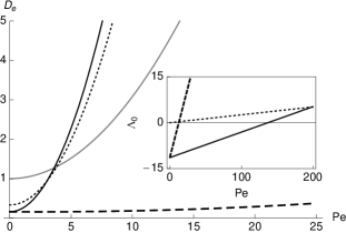
a)    b)

Figure 4: Effective diffusivity (inset: drift, $\Lambda_{0}$) against Pe calculated using asymptotic solutions to the Fokker-Planck approach. a) Poiseuille approximation (case I) for $\eta=0.007$ (solid line), $\eta=0.3$ (long dashed), $\eta=100$ (dashed) and the classical Taylor-Aris result (grey). b) Self-driven flow ($\tilde{p}_{x}=0$) using the coupled solution from case II (broad plumes; $\eta=0.007$). Mode 1 (long dashed) and mode 2 (dashed) are shown with the uncoupled limit (solid).

The figure reveals that low and high levels of gyrotaxis (measured by $\eta$) lead to behaviour akin to Taylor dispersion but intermediate levels dramatically reduce the impact of advection. This is because at these intermediate levels the cells form dense plumes in the centre of the tube so are not subject to the full range of flow speeds. On the other hand, intermediate gyrotaxis does lead to large amounts of swimming and flow induced drift relative to the mean flow, due to their central location. For small and intermediate $\eta$ the asymptotic results reveal that the drift changes sign for a non-zero Pe number. However, the asymptotic results for large $\eta$, are not strictly valid for small Pe. Nonetheless, one would expect the drift to change sign in a similar manner, such that all three curves intersect on the $y$-axis.

6.4 Algae in self-driven flow (weak coupling, $A\ll 1$)

Recall from section 3 that for self-driven flows there are two solutions: a simple mode 1 flow and a mode 2 flow with upwelling at the tube sides. To calculate the transport coefficients in these cases the definitions (74) are employed (since the flow solutions were all obtained for $\eta\ll 1$ and weak coupling, $A\ll 1$). With the same parameters as for the $\eta=0.007$ case in figure 4a, figure 4b plots the diffusivity and drift (inset). It is clear that the mode 1 results for these broad plumes are rather similar to those generated by Poiseuille flow. However, for the mode 2 solutions cells both drift and diffuse faster, likely due to the greater shear.

7 Discussion

In this paper, we derive exact expressions in the long-time limit for the mean drift and effective axial diffusion of an axisymmetric blob of biased, swimming microorganisms in a plume in a pipe flow driven by an external pressure gradient and the presence of the (negatively) buoyant cells. In the same limit, we find that the axial skewness of the cross-sectionally averaged cell distribution vanishes. The results are independent of the cell geometry, swimming behaviour and model used to represent the cell-flow interactions.

Explicit results for several useful cases are presented, from the Taylor-Aris limit to fully coupled gyrotactic spherical swimming cells (i.e. cells that drive the flow and whose swimming direction is biased by external and viscous torques). The expressions reveal the mechanisms for several competing effects and explain how these lead to diffusion and (positive or negative) drift through the tube. Fundamentally, the cells swim and, in the limit that they are very bottom heavy, they may swim mostly against a downwelling flow, leading to a negative drift relative to the mean flow. On the other hand, cells that are not bottom heavy act more like diffusing passive tracers, with no drift. In both these cases the cells diffuse as for Taylor-Aris dispersion. However, an intermediate degree of bottom heaviness leads to much more interesting behaviour. A balance between gravitational and viscous torques, a balance that will vary across the pipe flow, can lead the cells to form gyrotactic plumes, inducing further flow and self-concentration. These centrally focused plumes of cells can be strongly advected with the flow (i.e. faster than the mean flow) but will sidestep classical shear-induced Taylor-Aris dispersion; effective diffusion may be dominated by swimming diffusion even for large flow rates. It is clear that swimming behaviour leading to drift across streamlines can have a tremendous influence on cell transport in such systems.

The results are sufficiently general that they may easily be applied to other micro-organisms and taxes, such as chemotaxis in suspensions of bacteria swimming in flows in microfluidic chambers, or spermatozoa in vivo. In a subsequent paper we shall provide further explicit examples for non-spherical cells (behaviour influenced by the rate-of-strain tensor) and for additional swimming stresses for concentrated suspensions. Both these aspects will modify the plume structure and thus affect axial cell transport.

Work in progress is exploring how the theory can be applied to determine the qualitative form of the orientationally averaged cell swimming diffusion tensor for suspensions of gyrotactic cells from experiments. For a realizable experiment one must introduce dyed cells into a plume whilst maintaining a constant cross-sectionally averaged cell concentration. This may be achieved simply by momentarily switching from undyed to dyed cells at the input or using photoactivatable GFP for localized photolabelling of cells (Patterson & Lippincott-Schwartz 2002). Note that plume solutions for the various diffusion descriptions differ qualitatively for large Peclet numbers, and thus so must predictions for mean drift and effective diffusion. Hence, we aim to clarify the applicability of differing diffusion approximations in a general shear flow.

8 Acknowledgements

The authors gratefully acknowledge support from the EPSRC (EP/D073398/1).